Abstract
Floods are frequent hydro-meteorological hazards which cause losses in many parts of the world. In hilly and mountainous environments, floods often contain sediments which are derived from mass movements and soil erosion. The deposited sediments cause significant direct damage, and indirect costs of clean-up and sediment removal. The quantification of these sediment-related costs is still a major challenge and few multi-hazard risk studies take this into account. This research is an attempt to quantify sediment deposition caused by extreme weather events in tropical regions. The research was carried out on the heavily forested volcanic island of Dominica, which was impacted by Hurricane Maria in September 2017. The intense rainfall caused soil erosion, landslides, debris flows, and flash floods resulting in a massive amount of sediments being deposited in the river channels and alluvial fan, where most settlements are located. The overall damages and losses were approximately USD 1.3 billion, USD 92 million of which relates to the cost for removing sediments. The deposition height and extent were determined by calculating the difference in elevation using pre- and post-event Unmanned Aerial Vehicle (UAV) data and additional Light Detection and Raging (LiDAR) data. This provided deposition volumes of approximately 41 and 21 (103 m3) for the two study sites. For verification, the maximum flood level was simulated using trend interpolation of the flood margins and the Digital Terrain Model (DTM) was subtracted from it to obtain flooding depth, which indicates the maximum deposition height. The sediment deposition height was also measured in the field for a number of points for verification. The methods were applied in two sites and the results were compared. We investigated the strengths and weaknesses of direct sediment observations, and analyzed the uncertainty of sediment volume estimates by DTM/DSM differencing. The study concludes that the use of pre- and post-event UAV data in heavily vegetated tropical areas leads to a high level of uncertainty in the estimated volume of sediments.
1. Introduction
Hydrological disasters such as river floods and flash floods associated with extreme weather events have caused significant damage [1,2]. Methods that determine the impact of such disasters are generally well established. Flood hazard maps are created from hydro-dynamic models [3,4,5,6,7], and the flood intensity (such as maximum water height and flow velocity) is linked to the physical vulnerability of elements at risk using damage curves that are related to building of land use types [4,8,9,10,11,12,13]. While there are many studies that focus on the erosion process [14,15,16,17,18], relatively few have investigated the relation between erosion and sedimentation and the incurred damages and costs. Geomorphologists are well aware of muddy floods (e.g., [19]), but often consider it as an “offsite” (downstream) effect. The research efforts on the quantification of the damage and clean-up costs incurred by sediment deposition are much less than those that model the initiation and transportation processes.
Therefore, one of the remaining challenges is the inclusion of the effect of sediments in the flood risk analysis. Sediment deposition in built-up environments causes significant direct damage and indirect costs. Direct damage is to the contents of private and public buildings, to crops and other elements at risk that are destroyed by the sediments. The indirect costs are related to cleaning operations, unblocking drainage and sewage systems, and removal of sediments to prevent future flooding [20,21,22].
It is common to analyze the run out of landslides and debris flows with a range of models, to quantify the damage related to impact pressure against objects [23,24,25,26], but the losses related to clean-up of sediments are generally not considered.
Sediment deposition volumes depend on sediment detachment, transport, and deposition processes. Sediments are generated by different processes such as splash and flow detachment of particles from the soil surface, and landslides that move the entire soil body. Sediments are transported by runoff and floods, as well as mass movements (e.g., mudflows and debris flows). Within a catchment, these phenomena often occur at the same time during the triggering event; within a channel, various processes may occur alternatively. The energy of the flow determines how much material can be transported, and the environment determines what kind of material is actually available [27]. Moreover, in the process of entrainment, strong flashfloods and debris flows may erode substantial amounts of sediment from the riverbeds. The sediments from the erosion process consist of fine particles of sand size or smaller, while the materials generated by landslides and entrainment—depending on the type of materials available in the surrounding environment—are of a wide range of particle sizes, ranging from clay to large rocks and boulders. Additionally, tree debris may be an important component of the floods and debris flows in forested watersheds. Regardless of the sediment production mechanism, deposition occurs when the transport capacity of the flow is not sufficient to transport the material due to changes in velocity, which itself is caused by changes in slope, resistance to flow, or presence of obstacles [28,29,30,31].
Several approaches are reported in the literature for quantifying sediment deposition, such as using historical archives [32,33,34], participatory mapping [35], field surveying [36,37], optical remote sensing in combination with pre-event Digital Elevation Models (DEMs) [38,39,40,41], generation of pre- and post-event DEMs [42,43,44,45,46], and modelling [34,36,38]. In practice, a combination of different methods is often used (e.g., [35]). The quantification of the height and volume of loose materials is also done for other environments. For example, [47] reviewed a number of empirical relationships between tephra accumulation depth and tephra volume and duration of clean-up operations.
One of the common methods for quantifying geomorphological change, such as erosion and sediment deposition, is to produce DEMs of Difference (DoDs). DoDs are the result of subtracting successive DEMs captured before and after an event [41]. This is frequently used by researcher; for instance, Brasington et al. [48] developed and compared DEMs for a river in Scotland using digital photogrammetry and high-resolution GPS ground surveys to monitor erosion and deposition processes. Fuller et al. [49] constructed DEMs for a river in England using theodolite surveys and calculated the annual sediment transfer volume by differencing the DEM surfaces. Milan et al. [40] used a high-resolution 3D laser scanner to produce detailed DEMs and assess the erosion and deposition volumes in a river in Switzerland.
The quality of a DEM generated from surveys is directly influenced by the accuracy of survey points and the survey strategy [50]. It should be noted that uncertainty in DEMs affects the DEM differencing and some approaches were developed to cope with this, such as calculating an average uniform error across DEMs [39], accounting for local differences in DEM errors [40,48], and performing a spatially distributed error estimation related to local topographic variability across DEMs [50,51,52].
The aim of this research is to quantify the sediment deposition of flashfloods and debris flows in a tropical area with dense vegetation—where a high-quality pre-event DTM is missing—as a basis for the assessment of sediment clean-up costs. These cost calculations can be used as an important component in the risk analysis of sediment deposition. It is intended to investigate the challenges and limitations associated with quantification of sediment deposition in areas where dense vegetation hinders construction of accurate DTMs. The research was carried out in Dominica, after the occurrence of flash floods and debris flows triggered by 2017′s Hurricane Maria.
2. Study Area
Dominica is located in the Eastern Caribbean Sea between the French islands of Guadeloupe and Martinique. It is 46 km in length and it has an area of about 750 km2. The island is predominantly covered by rainforest [53]. The topography is rugged, and the geology is volcanic with extensive ignimbrite rocks which are easily eroded and weather rapidly in the wet tropical environment [54,55], leading to thick residual soils [56,57,58]. The environmental conditions, combined with tropical storms, led to the frequent occurrence of mass movements [59]. Most communities are located at the mouth of rivers, which makes them exposed to (flash) floods and debris flows. The island communities are connected through a circular road network running along the coast, and a single diagonal road connecting the capital Roseau with the Douglas Charles airport in the north east. The island has a hot and humid tropical climate. The dry season runs from December to May and the wet (hurricane) season from June to November; the average annual temperature is 27.5 °C [60]. The meteorological stations at the Douglas Charles and Canefield airports reported annual average rainfalls of 2650 mm and 1760 mm, respectively [60].
This research is focused on two villages which were heavily affected by debris flows during the 2017 Hurricane Maria: Coulibistrie, located at the coast (N15.46 W61.45) on the west side of the island, and Pichelin, located inland (N15.26 W61.33) in the southern part of the island (Figure 1). The yellow polygons in Figure 1 are the same as the blue polygons in Figure 5.
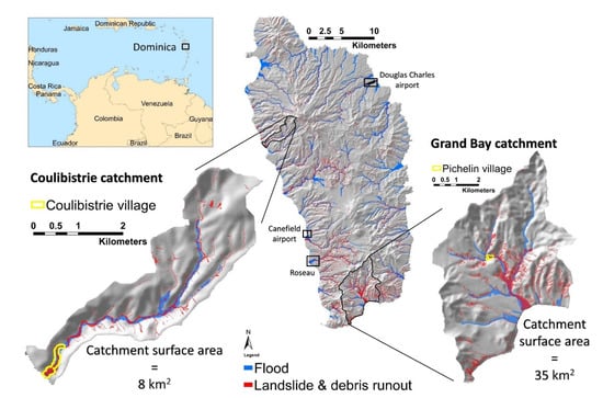
Figure 1.
Location of study areas (Coulibistrie and Pichelin) shown on a hill-shading map of Dominica. Floods are indicated in blue; landslides and runouts are indicated in red. The enlarged images are the hill-shading maps of the two catchments overlaid by floods and landslides and debris runout. The floods are simulated on a 20 m resolution, while the landslides and debris flows are derived from satellite image interpretation (see Charim.net).
Hurricane Maria impacted the island on 18 September 2017, after it developed quickly from a tropical storm to a category 5 hurricane. Strong winds damaged the tropical vegetation. Storm surges affected the coast. Intense rainfall and the uprooting of trees triggered close to 10,000 landslides. Debris flows and flashfloods occurred in nearly all watersheds [61]. Out of the total of 31,352 homes, 15% were fully destroyed, and 75% suffered different levels of partial damage [62]. Large amounts of sediments and debris were generated by erosion and landslide processes [62]. Shoreline infrastructure was damaged by coarse sediment and tree debris discharged into the sea and transported back onto the coastline by the storm surge [63,64]. Sediments and tree debris carried by floods filled up the channels and blocked bridges and culverts, intensifying the flooding situation upstream, causing countless roadblocks in parts of the island and damage to facilities and infrastructure [65,66] (Figure 2). Table 1 provides information regarding the cost of cleaning operations.
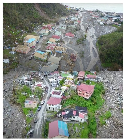
Figure 2.
Above: oblique view of Coulibistrie village immediately after Hurricane Maria: sediment deposition has a high spatial variability and it is a mixture of sediments, rocks and boulders, and tree debris (UAV video available at https://www.youtube.com/watch?v=QTuymqtkfig&t=62 (accessed on 5 May 2021)). Below: oblique view of Pichelin village, taken shortly after the event. The village is located between two valleys that were filled with debris (UAV video available at https://www.youtube.com/watch?v=1aaPY-309Ko (accessed on 5 May 2021)).

Table 1.
Post hurricane Maria damage, losses, and recovery needs (as of 3 November 2018). (Sources: Dominica’s Ministry of Public Works; [62]).
3. Methodology
The methodology of this research is schematically represented in Figure 3. All GIS operations of this study were performed using ArcMap 10.8. Two approaches were followed as the main methods for sediment deposition quantification. Both approaches are based on differencing pre- and post-event DEMs. Deposition quantification results were verified using three approaches. Estimation of deposition height is crucial for assessing the risk imposed by sediment deposition specially in built-up environments.
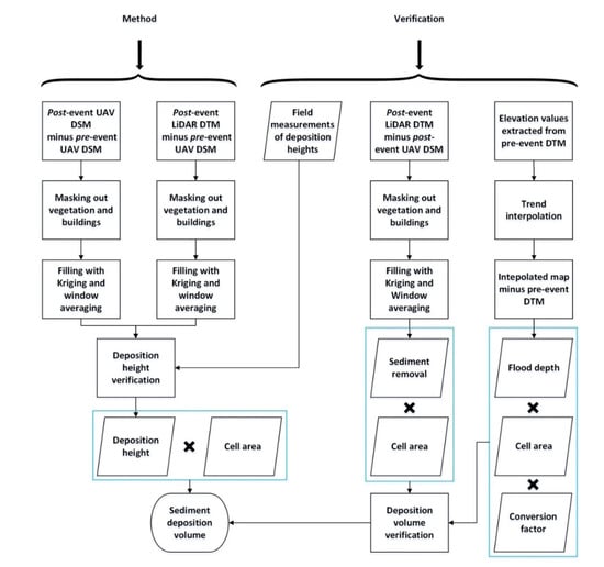
Figure 3.
Schematic representation of research methodology. Specifications of pre- and post-event UAV DSM and LiDAR DTM are given in Table 2.
3.1. Field Data Acquisition
Sediment deposition height was measured in the field, during the first two weeks of October 2018, from the marks on the walls of buildings (Figure 4a). At some locations where sediments inside buildings were still in place (Figure 4b), the actual height of deposition was measured. All measurements were made relative to the buildings’ surrounding ground level. Deposition height estimations were checked by interviewing local residents. In some cases, traces of the maximum flood level were visible on walls, but it was not clear whether these represented water level or deposition traces. Videos and photographs taken during and shortly after the event were also used to verify the deposit depths. Deposition height was determined at 30 locations in Coulibistrie and 12 locations in Pichelin (Figure 5).
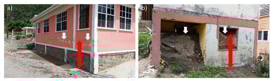
Figure 4.
(a) Sediment deposition height measured from marks on the walls. The white arrows show the deposition/flooding marks on the wall and the red arrow is the measured deposition/flooding height. (b) Sediment deposition height measured from remaining sediments inside a building. The white arrows show the deposition surface inside the building and the red arrow is the measured deposition height.
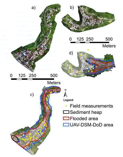
Figure 5.
(a) Pre-event orthophoto of Coulibistrie. (b) Pre-event orthophoto of Pichelin. (c) Post-event orthophoto of Coulibistrie with field data collection points. (d) Post-event orthophoto of Pichelin with field data collection points; background is a combination of pre-event (transparent) and post-event orthophotos. Note that post-event DSM data do not completely cover the flooded area for Pichelin.
3.2. Remotely Sensed Data
Zekkos et al. [67] collected pre-event UAV data approximately three weeks before landfall of Hurricane Maria in Dominica at nine locations. They determined the uncertainty in their DEMs by surveying 13 to 40 ground control points (GCPs) per area. The number of GCPs was decided based on the size of each site. Zekkos et al. [67] used the GCPs as checkpoints and calculated the root mean square error (RMSE) as vertical accuracy (Table 2). Schaefer et al. [68] performed UAV surveys four months after hurricane Maria in different parts of Dominica to investigate the topographical changes. They assessed the uncertainty in their DEMs using the pre-event UAV data from Zekkos et al. [67] as reference. Schaefer et al. [68] did not lay out any GCPs, due to safety considerations in accessing survey areas on foot. They matched their data with the data collected by Zekkos et al. [67] in three dimensions by comparing the point clouds or the GCPs derived from pre-event data. The comparison was made for unchanged features such as roofs and roads. Schaefer et al. [68] applied the resulting transformation matrix to the whole cloud. They assessed the DSMs accuracy (Table 2) by creating profiles in ArcGIS using the Stack Profile tool along the airport runway or roads and comparing in a Python script.
The flight height for UAV imagery was aimed at 50 m above ground level; however, it was varied between survey sites depending on the surrounding area. Pre-event imagery was captured using a GJI Phantom 4 Pro. Post-event surveys were performed using a DJI Phantom 3 (P3) and a DJI Phantom 4 (P4). Schaefer et al. [68] provided us with pre- and post-Maria Digital Surface Models (DSMs) and orthophotos for Coulibistrie and Pichelin. Dominica’s National Physical Planning Department provided post-Maria LiDAR DSM and DTM data which were obtained through a World Bank funded project [69]. They also provided post-Maria UAV orthophotos (Table 2). It is clearly shown in Figure 5 that the areas covered by pre- and post-event images were not the same, and that the presence of vegetation in the pre-event images hampered the acquisition of accurate pre-event elevation data for certain areas.
Both pre- and post-event UAV DSMs were resampled with bilinear technique to 0.5 m resolution to make the comparison with LiDAR data possible. In order to evaluate the matching of the pre- and post-event DSMs, we checked the horizontal alignment and elevation for undamaged roads and buildings. Particularly, the elevation of concrete building rooftops extracted from the same pre- and post-event UAV DSMs were compared. The two DSMs matched very well with regard to horizontal alignment; however, there were small differences in terms of vertical elevation. The RMSE of elevation for undamaged locations was 0.23 m for Coulibistrie (based on 67 points) and 0.38 m for Pichelin (based on 10 points).
The post-event LiDAR data were acquired through an aerial topographic and bathymetric LiDAR survey for Dominica using the OptechGalaxy T1000 LiDAR system with an integrated PhaseOne-iXU-RS1000 camera. The flying height was 1830 m above sea level. The uncertainty of LiDAR DEM was assessed using ground survey values at 284 check points in three location: Douglas Charles International airport, Portsmouth, and Sineku/Kalinago. The accuracy was estimated by calculating the RMSE between individual LiDAR points and the check points (Table 2). LiDAR DTM was produced several months after hurricane Maria, and cleaning operations and sediment removal had already been carried out for most of the areas. The LiDAR operation took several months, and it is not known when exactly the DTMs of the two villages were obtained. Nevertheless, it can be used to give an indication of the volume of sediments removed.
ALOS PALSAR and SRTM DTMs were obtained and resampled to 10 m using bilinear technique. The bilinear resampling operations of this research were performed in ArcMap 10.8 which uses the four nearest cell values to determine the value on the output raster [70]. The original data type of ALOS PALSAR and SRTM is integer. This was changed to floating data type before resampling to get more continuous datasets.
Table 2.
Specifications of remote sensing datasets. The hurricane occurred on 18 September 2017.
Table 2.
Specifications of remote sensing datasets. The hurricane occurred on 18 September 2017.
| Data | Time of Acquisition | Resolution (m) | Vertical Accuracy (m) | Source |
|---|---|---|---|---|
| SRTM DTM | February 2000 | 30 | ≈ 9.00 | US National Aeronautics and Space Administration |
| ALOS PALSAR DTM | March 2011 | 12.5 | ≈ 5.00 | Japan Aerospace Exploration Agency |
| UAV pre-event DSM and orthophotos | 22 August to 3 September 2017 | 0.02 | 0.10 | University of Portsmouth [67,68] |
| UAV post-event DSM and orthophotos | 25 January to 2 February 2018 | 0.04 | 0.10 | University of Portsmouth [68] |
| LiDAR post-event DSM and DTM | 19 February to 5 May 2018 | 0.50 | 0.05 | Dominica’s National Physical Planning Department [69] |
3.3. Deposition Height Estimation
We made use of pre- and post-event DTMs, depicting the bare terrain surface, and DSMs, that represent the elevation including all vegetation and human-made objects. The disadvantage of DSMs derived from UAV data is that they do not allow to create DTMs, or bare surface models due to presence of obstacles (e.g., vegetation, buildings, etc.). Therefore, if the study area is densely vegetated before the occurrence of the extreme event, it is only possible to measure the difference for those areas that were bare before the event, such as the riverbeds.
The height of sediment deposition after hurricane Maria was determined by subtracting the UAV pre-event DSM from the UAV post-event DSM. The outcome of this differencing will be named “UAV-DSM-DoD” from here onwards. The cell values of UAV-DSM-DoD inside buildings and in vegetated areas were masked-out. The elevation difference for the masked-out UAV-DSM-DoD was analyzed using two approaches:
- UAV-DSM-DoD was converted to points and spatially interpolated with Gaussian Kriging to cover the whole study area. Kriging produces unbiased values with minimum variance [71], and it is based on regionalized variable theory (RVT) which is capable of describing the variation in sediment accumulation [36]. Four Kriging models (Exponential, Circular, Spherical, and Gaussian) were applied and compared. The Gaussian model was used as it provided the best semivariogram fit. The masked-out parts were filled in using the corresponding parts of the interpolated raster.
- A three-by-three smoothing filter (window average) was used repeatedly until the masked-out areas in UAV-DSM-DoD was filled [72,73].
Deposition height was also determined by subtracting the UAV pre-event DSM from the LiDAR post-event DTM. This provides a minimum range for sediment deposition. Before performing the subtraction, the buildings and vegetated areas in UAV pre-event DSM were masked out and filled in with the two above-mentioned approaches. The outcome of this differencing will be named “LiDAR-DTM-DoD” from here onwards.
The filling process was done under the assumption that water and sediment entered the buildings, and below the canopy of trees that were still standing. This was observed in the field, and in a video taken during the event. It is possibly that not all buildings had been filled with sediment to the same level as the outside, but it was not possible to determine this afterwards. Leaving the masked buildings out of the calculation of volume would present an underestimation, while assuming that all buildings have sediment inside, is likely an overestimation of the volume. The sediment height data per cell were multiplied by the cell area (0.25 m2) and summed up to obtain the total deposition volume.
For the sake of conformity, all the analysis for this research were performed within an overlapping area defined by the UAV-DSM-DoD for both Coulibistrie and Pichelin (Figure 5c,d).
3.4. Verification
3.4.1. Field Measurements
The deposition height data points, determined in the field in Coulibistrie and from online videos recorded immediately after the event, were compared with the deposition height values extracted from deposition height maps (generated in Section 3.3) for the same locations. This comparison was not performed for Pichelin as only three of the measured points fall within the extent of UAV-DSM-DoD (see Figure 5d).
3.4.2. Volume of Removed Sediments
The volume of removed sediments can be considered as a lower limit for deposition volume, but it does not represent the entire sediment deposition. This was calculated by subtracting the UAV post-event DSM from the LiDAR post-event DTM. The outcome of this differencing is referred to as “LiDAR-DSM-DoD” from here onwards. The temporal gap between these two post-event products is maximum three months. LiDAR-DSM-DoD is useful for estimating the volume of the removed sediments and also identifying the locations where sediment removal has occurred. The same masking-out and filling procedure (explained in Section 3.3) was followed to correct the UAV post-event DSM for buildings and vegetated areas before subtraction.
The sediments collected during the cleaning and sediment removal operations in Coulibistrie were piled up in a dumpsite at the shoreline (Figure 5c). The volume of this dumpsite is a good indicator for the volume of sediments removed in Coulibistrie; however, it does not represent the total volume of deposited sediments as, in many places within the village, sediments are still left in place, and part of the dumpsite was eroded by the sea. The elevation of the dump is captured by the post-event LiDAR DSM. The Google Earth images show that this location had an elevation above sea level before the event. However, the flow of water during hurricane has reduced this elevation by washing off some soil into the ocean. Nevertheless, it was assumed that the original elevation of this location was zero (sea level); therefore, the elevation shown by the post-event LiDAR DSM was considered as the absolute height. At some locations on the dumpsite, the LiDAR DSM showed sudden jumps in elevation. This could be caused by vehicles and machinery that are placed there, or the removal of tree debris from the dumpsite. These were also masked out and filled using the same filling approaches.
3.4.3. Trend Surfaces
The flooding surface during the event can be simulated by fitting a trend surface to the points located on the boundary of flooded area where the flood depth is zero. Spatial trend interpolation is a suitable tool for this purpose. The trend interpolation fits a smooth surface to the input points using a polynomial function. The trend surface captures the coarse-scale patterns in the data and does not show sudden changes [74].
The boundary of flooded area was digitized for each village with a polygon using the traces on the ground visible in the orthophotos and also the online UAV videos recorded during and shortly after the event (Figure 5). Some points were added on the edge of these polygons. The elevation was obtained from pre-event DTM for these points. A high-resolution pre-event DTM for the entire area was not available, as most of these areas were covered by vegetation before the event. Therefore, three pre-event DTMs were generated by combining the elevation values from pre-vent UAV DSM for bare surfaces in the pre-event situation with three products: the post-event LiDAR DTM for the areas where there were buildings and/or vegetation, masked out pre-event UAV DSM (for buildings and vegetation) filled with Kriging interpolation, and the same masked out map filled with window averaging.
Trend analysis were also performed using pre-event ALOS PALSAR and SRTM DTMS to see if freely available but relatively coarse-resolution datasets would give meaningful estimates compared to the high-resolution datasets.
The extracted elevation values of the flood boundaries were used to create trend surfaces with first-, second-, and third-order polynomial interpolations. Flood depth was calculated by subtracting the DTMs from interpolated surfaces. The generated maps show negative values at some locations where the terrain features have greater elevation compared to the trend surfaces. At these locations, the flooding depth was set to zero. The maximum flood depth map was multiplied by its cell area (0.25 m2) and summed to obtain the total flood volume. This was converted to total sediment deposition volume using the volumetric sediment concentration rates reported in the literature ranging from approximately 40% for mudflows to 80% for debris flows [75,76,77]. The results give an indication of the maximum volume of sediments that could have been deposited.
Figure 6 provides a graphical summary of the various methods applied to estimate the sedimentation volumes in forested areas.
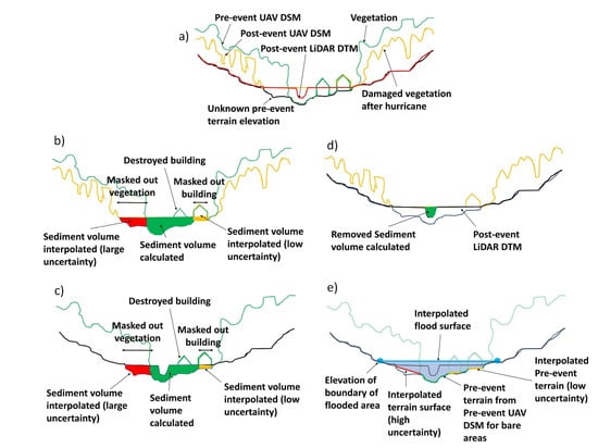
Figure 6.
Illustration of the methods applied for estimation of sedimentation volumes from pre-event UAV DSM, and post-event UAV DSM and LiDAR DTM. (a) Cross section of a valley with vegetation and buildings showing the elevation of the various elevation data sources, and the unknown pre-event topography. (b) Calculation of sediment volume from pre-event UAV DSM and post-event UAV DSM, using a method to interpolated thicknesses in areas occupied by vegetation or buildings. (c) Calculation of sediment volume from pre-event UAV DSM and post-event LiDAR DTM, using a method to interpolated thicknesses in areas occupied by vegetation or buildings. (d) Calculation of the removed sediments from the difference between the post-event LiDAR DTM and post-event UAV DEM. (e) Calculation of the maximum flood level, by establishing the elevation of the sides of the affected area on the LiDAR DTM following by trend surface interpolation, and reconstruction of the pre-event topography from the pre-event UAV DSM and interpolation in masked areas of vegetation and buildings.
4. Results
4.1. Deposition Height Estimation
Figure 7 presents the deposition height maps for Coulibistrie and Pichelin generated from UAV-DSM-DoD and LIDAR-DTM-DoD. As it can be seen from the histograms the two approaches used for filling the masked buildings and vegetation (Kriging and window average) produced very similar results. Total deposition volumes are given in Table 3.
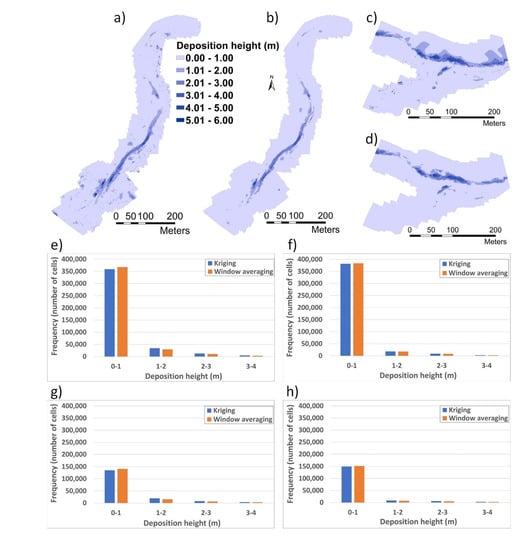
Figure 7.
(a) Coulibistrie UAV-DSM-DoD filled with window averaging. (b) Coulibistrie LiDAR-DTM-DoD filled with window averaging. (c) Pichelin UAV-DSM-DoD filled with window averaging. (d) Pichelin LiDAR-DTM-DoD filled with window averaging. (e) Histogram comparing the cell values of UAV-DSM-DoD for Coulibistrie filled with the two approaches (Kriging versus window averaging). (f) Histogram comparing the cell values of LiDAR-DTM-DoD for Coulibistrie filled with the two approaches. (g) Histogram comparing the cell values of UAV-DSM-DoD for Pichelin filled with the two approaches. (h) Histogram comparing the cell values of LiDAR-DTM-DoD for Pichelin filled with the two approaches.
Table 3.
Sediment volume estimations (all values are in 103 m3). The sediment removal volumes and deposition volumes from trend analysis are stated as intervals.
4.2. Verification
4.2.1. Field Measurements
The collected deposition height data in the field range between 0.3 and 2.3 m for Coulibistrie and between 1.1 and 3 m for Pichelin. Figure 8 shows the comparison between the field data points and the extracted deposition height values from UAV-DSM-DoDs and LiDAR-DTM-DoDs for the same locations.
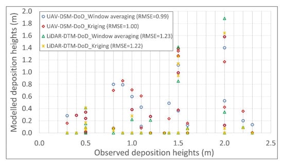
Figure 8.
Observed deposition heights versus modelled deposition heights for 30 locations of data collection in Coulibistrie. RMSE between observed and modelled values per method is given in the legend.
4.2.2. Sediment Removal
The results of comparing post-event UAV DSM with the post-event LiDAR DTM (LiDAR-DSM-DoD) are shown in Figure 9. This can be used to estimate the depth and volume of sediment removal after the event and to analyze post-event erosion. The difference between the two filling approaches is again limited. Contrary to what was expected, the LiDAR-DSM-DoD for Pichelin does not show significant sediment removal (Figure 9b), because the UAV and LiDAR data were both acquired in this area several months after the event, when the removal activities had already taken place. The volumes of removed sediments are given in Table 3.
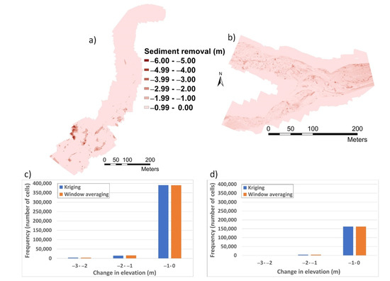
Figure 9.
(a) Coulibistrie LiDAR-DSM-DoD filled with window averaging. (b) Pichelin LiDAR-DSM-DoD filled with window averaging. (c) Histogram comparing the cell values of Coulibistrie LiDAR-DSM-DoD filled with Kriging and window averaging. (d) Histogram comparing the cell values of Pichelin LiDAR-DSM-DoD filled with Kriging and window averaging.
4.2.3. Trend Surface Analysis
For trend surface analysis, the pre-event DTM was generated using the approach explained in Section 3.4.3. Figure 10 shows the reconstructed pre-event DTMs for Coulibistrie and Pichelin where the masked-out vegetation and building areas were filled-in with the elevation values from the post-event LiDAR DTM. Comparing the three constructed pre-event DTMs shows that the map filled with LiDAR DTM data generally has lower values than those interpolated with Kriging or window averaging. The cell values of the post-event LiDAR DTM in vegetation and building areas which are located within flooded area do not represent the pre-event topography since they were affected by sedimentation during the event. Nevertheless, the LiDAR DTM data show the actual terrain elevation of the ground surface, while the elevation values produced by Kriging and window averaging are the artifacts of simulations. The errors are the highest in those locations which were covered by vegetation prior to the event, and where deposition of sediments took place (See Figure 6).
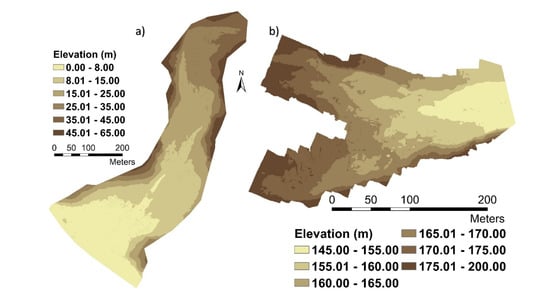
Figure 10.
(a) The generated pre-event DTM for Coulibistrie (filled with LiDAR DTM). (b) The generated pre-event DTM for Pichelin (filled with LiDAR DTM).
Flooding depth was simulated using the first-, second-, and third-order trend interpolations. The simulated flood elevation layers were compared with the available images and videos captured during and after the event. It was inferred that the results of the third order trend interpolation represent the real situation best, and the first and second order trend analysis results were discarded. The flood depth maps were generated by subtracting the pre-event DTM from the flood height map. Two of the generated flood depth maps are presented in Figure 11a,b.
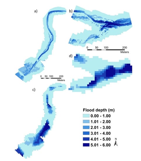
Figure 11.
(a) Flood depth map for Coulibistrie: 3rd order trend surface minus pre-event DTM filled with LiDAR DTM. (b) Flood depth map for Pichelin: 3rd order trend surface minus pre-event DTM filled with LiDAR DTM. (c) Flood depth map for Coulibistrie: 3rd order trend surface minus pre-event ALOS PALSAR DTM. (d) Flood depth map for Pichelin: 3rd order trend surface minus pre-event ALOS PALSAR DTM. For brevity the maps generated with SRTM DTM are not presented here.
In order to evaluate the effect of using a globally available, but more coarser resolution DEM such as ALOS PALSAR or SRTM, also these were used in combination with the flood elevation layer. The flooding depth patterns are vague (Figure 11c,d). This highlights the requirement of good quality pre-event DTMs for trend surface analysis. The generated flooding depth maps were used to calculate the total sediment deposition volume (Table 3).
5. Discussion
UAV and LiDAR data were used to produce DoDs as a measure of sediment deposition height. An ideal situation is when the pre- and post-event data are captured immediately before and after the event (e.g., [78]); however, this occurs rarely. In this study the UAV pre-event DSM was captured a few weeks before the hurricane, while the UAV post-event DSM was captured over three months after the event. This is sufficient time for growth of vegetation, some repairing or demolishing of buildings and infrastructure, and removal of sediments. Therefore, the positive and negative values in UAV-DSM-DoD include these effects. Kriging has shown a better performance for DEM construction compared to other interpolation methods [79]. However, a complicating issue was that both filling approaches are very much influenced by the cells at the edge or close to the edge of the masked-out parts, and the real deposition height inside these masked-out parts might be quite different from the one at the edges. For instance, the vegetation is mostly located on sloping terrain, and sediment deposition may be quite different along the boundaries of the masked-out vegetation. When the vegetated areas are masked-out, the edges of masked-out parts are located just beside the channel where a large amount of sediment was deposited. These large values of deposition height are used by Kriging interpolation and window average function to calculate the deposition height on the surrounding steep slopes (vegetated areas) which may be overestimated.
In order to increase the accuracy of modelled deposition heights, a detailed field survey is needed [80]; however, this may not be feasible in many cases due to logistical problems or lack of required facilities. The deposit heights measured in the field are generally greater than those from the UAV-DSM-DoDs and LiDAR-DTM-DoDs, as shown by the large RMSE values in Figure 8. The smallest differences were obtained for those locations where sediments were left inside abandoned buildings. The field data points where measurements were based on marks on walls, give too high value, indicating that the flood level was marked instead of the level of sediment deposits, which was later removed.
After an event, the deposition is a mixture of sediments, large rocks and boulders, tree logs, and other debris [81]. Additionally, erosion occurs in the middle of channel. The sediment deposition surface is not flat, and the sediment height has a high spatial variability. The marks on the walls and the remaining sediments inside buildings do not indicate a flat surface. The data gathered by interviewing local residents contain some uncertainties as well. Field measurements were carried out in October 2018 which is more than a year after the event. Over the period of one year some other processes such as erosion and sediment removal operations were in progress as well. Due to all these factors sediment deposition is not easy to be characterized in the field and it comes with some uncertainties.
It is essential to take note of the limitations regarding trend analysis. Determining the flooded area boundary is difficult at places where the quality of the images and orthophotos is poor. However, the most important aspect is the quality of the pre-event DTMs. If there are only coarse-resolution DEMs available, the results will be much less reliable. If only pre-event DSMs are available, the use of the Kriging interpolation and window averaging lead to significant uncertainties.
Table 3 presents the calculated sediment deposition volumes using the different methods presented before. The calculated deposition volumes from UAV-DSM-DoD filled with Kriging and window averaging (items 1 and 2 in Table 3) are very close. Summation of deposition volumes from LiDAR-DTM-DoD (items 3 and 4 in Table 3) and sediment removal volumes from LiDAR-DSM-DoD (item 5 in Table 3) is almost equal to deposition volumes from UAV-DSM-DoD; which verifies our estimations. The volume of the sediment deposited heap at the shoreline near Coulibistrie and the sediment removal volumes from LiDAR-DSM-DoD provide a lower limit for sediment deposition. They show smaller values in Table 3 which approves the fact that a substantial amount of deposited sediment was still not removed at the time of capturing the LiDAR data. The sediment heap volume is higher than the volume calculated from sediment removal volume. This is because the UAV post-event DSM (which is used for calculation of LiDAR-DSM-DoD) was captured three months after the event and within this period some sediments were already collected. Therefore, the LiDAR-DSM-DoD does not reflect the total amount of sediment removal. It may be that the volume of the sediment heap is overestimated since it was assumed that the elevation of that location before the event was zero, which may not be realistic.
The deposition volumes from the trend analysis are stated as intervals according to the range of sediment concentration rates for mudflows and debris flows mentioned in Section 3.4.3. Trend analysis results in a wide range of deposition volumes, and the method is very sensitive to the quality of the pre-event DTM, the reconstruction of the flooded area, and the sediment concentration values. However, it may be the only method possible when in situ investigation is not feasible or when post-event UAV/LiDAR data cannot be obtained. Trend analysis with the two constructed DTMs (items 7 and 8 in Table 3) provide a reasonable range of deposition volume which is in agreement with the volumes from UAV-DSM-DoD (items 1 and 2 in Table 3). The generated DTM with post-event LiDAR DTM (item 8 in Table 3) provides the closest range of deposition volume. Trend analysis with low-resolution DTMs obtained from ALOS PALSAR (12.5 m) and SRTM (30 m) (items 9 and 10 in Table 3) gave unrealistic flooding patterns and exaggerated deposition volumes. This is caused by the low quality and coarse resolution of these datasets. Despite the uncertainties, trend analysis with such open access DTMs is useful for obtaining an upper limit for deposition volume when high-quality data are not available.
Quantification of sediment deposition in densely vegetated areas is associated with significant challenges and uncertainties, as discussed above. The major issue for our case was the lack of a high-quality pre-event DTM, which makes it different from studies that have access to such data (e.g., [39,43,45,46,48]). This study represents a common practical application as in many cases high quality pre-event DTMs are not available, especially in developing countries. For analysis of DEM uncertainty, an accurate dataset needs to be available to be considered as the baseline (e.g., [39,48,52]. However, our study sites had no reference data or the reference data were significantly altered due to hurricane damage.
The uncertainty of our DEMs was estimated considering the LiDAR DSM as the most accurate dataset. The elevation of unchanged features (buildings) was extracted from pre-event UAV DSM, post-event UAV DSM, and the LiDAR DSM. Figure 12 shows a comparison between elevation values of LiDAR DSM and that of UAV DSMs. The calculated RMSEs are smaller than 0.5 m which indicates a relatively slight uncertainty.
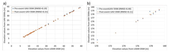
Figure 12.
(a) Elevation values of LiDAR DSM versus that of UAV DSMs for Coulibistrie. The RMSE between these datasets are given in legend. The elevation values were extracted from 67 points. (b) Elevation values of LiDAR DSM versus that of UAV DSMs for Pichelin. The RMSE between these datasets are given in legend. The elevation values were extracted from 10 points.
More than half of the cells of each product (excluding the sediment heap) were made by masking out and filling vegetated areas and buildings using Kriging interpolation or window averaging (Table 4), which indicates the high uncertainty of these products. This affects the total sediment deposition and sediment removal volumes calculated from UAV-DSM-DoD, LiDAR-DTM-DoD, and LiDAR-DSM-DoD but it has slight effect in calculation of deposition volume from trend analysis. Sources of uncertainty for our methodology and their degree of influence are summarized and presented in Table 5.
Table 4.
The percentage of filled (or masked-out) area for different products of DTM and DSMs analysis.
Table 5.
Sources of uncertainty and their degree of influence on results.
6. Conclusions
The quantification of sediment deposition is an important step in the assessment of the indirect risk of floods and debris flows. Digital Elevation Models that represent the situation before and after the flood event are one of the most important data sources for such analysis. The optimal approach for quantification of sediment deposition is calculating the elevation difference from pre- and post-event LiDAR DTMs. However, LiDAR is expensive and also difficult to obtain in areas with a lot of cloud cover, as in Dominica. The LiDAR survey for the entire country was never completed as the center of the island was under continuous cloud cover during the period of the LiDAR survey. Producing UAV data shortly after an event is cheap and feasible. Generating a difference map using pre-event LiDAR and post event UAV DSM is a feasible approach providing accurate results.
DEMs generated from pre- and post-event UAV surveys are an inexpensive alternative for this type of analysis. However, they are less useful in environments with dense vegetation. This study demonstrated an approach to generate sediment thickness maps from multi-temporal DSMs by masking out vegetated areas and interpolation of the data from their surroundings.
Rapid mapping of flooding boundaries with optical images and a pre-event LiDAR DTMs to generate trend surface is the next optimal approach. This research introduced an approach for the quantification of sediment deposition when post-event data are not available, and fieldwork cannot be carried out.
The analysis proved to be challenging and associated with high uncertainties. The most challenging was the reconstruction of the pre-event topography from UAV data for vegetated areas. Using high resolution pre-event DTM is beneficial for accurate estimation of deposition volume from trend analysis. However, it occurs very rarely that high quality Digital Terrain Models are available for a specific location before an extreme event.
A reliable assessment of sediment deposition volume requires a large number of field measurements with good distribution over the entire study area. The quality of elevation change analysis with UAV and LiDAR products can be improved by inspecting the buildings and vegetated areas in the field, soon after the event, in order to have a better estimate of deposition height. It is important to inspect in the field the locations where the boundary of flooded area is unrecognizable from aerial images. Despite all the challenges and uncertainties, analysis of UAV and LiDAR products has the advantage of using spatially distributed measurements of elevation differences.
The outcomes of this research can be used for assessment of the risk imposed by sediment deposition in built-up environments and the design of relative mitigation measures. Determining the volume and pattern of sediment deposition can assist policy makers to prepare a more efficient post-disaster recovery plan and limit the costs and damages.
Although not investigated in the scope of this paper, the results from this study can be used to calibrate spatial flash flood models for maximum water level and sediment/debris volume. A post-disaster flood hazard assessment should be based on updated DEMs since the future flood and mass movement processes will be significantly affected by the sedimentation from the past event.
Although UAV photogrammetry is not desirable for capturing ground surface in vegetated areas, without UAV data this analysis would not be possible. Acquiring UAV images after an event of this magnitude can be extremely helpful. Although the areal coverage is limited, organizations can focus on the most affected areas. This would assume that a DSM is available from pre-disaster conditions. It is very useful for Dominica to have a LiDAR DTM at this point but, for several areas, the DTM includes cleaning operation, so the surface does not represent pre-disaster conditions. Additional UAV data would help in these areas.
Author Contributions
Conceptualization, S.E., V.J., C.v.W. and D.P.S.; methodology, S.E., V.J., C.v.W. and D.P.S.; validation, S.E.; formal analysis, S.E.; data curation, S.E., V.J., C.v.W. and D.P.S.; writing—review and editing, S.E., V.J., C.v.W. and D.P.S. All authors have read and agreed to the published version of the manuscript.
Funding
This research received no external funding.
Institutional Review Board Statement
Not applicable.
Informed Consent Statement
Not applicable.
Data Availability Statement
Restrictions apply to the availability of these data. Data was obtained from University of Portsmouth and Dominica’s National Physical Planning Department, and are available from the authors with the permission of the mentioned parties.
Acknowledgments
We wish to acknowledge Dominica’s Physical Planning Division for their support during our field work in Dominica. We thank Annie Edwards and Lynn Baron for providing UAV images and facilitating collection of field data. We also gratefully acknowledge Martin Schaefer and Bastian van den Bout for providing valuable comments and inputs. Finally, we thank many interviewees who contributed to this research by sharing their experiences regarding hurricane Maria.
Conflicts of Interest
The authors declare no conflict of interest.
References
- Vos, F.; Rodríguez, J.; Below, R.; Guha-Sapir, D. Annual Disaster Statistical Review 2009: The Numbers and Trends; Centre for Research on the Epidemiology of Disasters (CRED): Brussels, Belgium, 2010. [Google Scholar]
- Guha-Sapir, D. EM-DAT: The Emergency Events Database; Universite catholique de Louvain (UCL)—CRED: Brussels, Belgium, 2017. [Google Scholar]
- Islam, M.M.; Sado, K. Development of flood hazard maps of Bangladesh using NOAA-AVHRR images with GIS. Hydrol. Sci. J. 2000, 45, 337–355. [Google Scholar] [CrossRef]
- Freni, G.; La Loggia, G.; Notaro, V. Uncertainty in urban flood damage assessment due to urban drainage modelling and depth-damage curve estimation. Water Sci. Technol. 2010, 61, 2979–2993. [Google Scholar] [CrossRef] [PubMed]
- Kourgialas, N.N.; Karatzas, G.P. Flood management and a GIS modelling method to assess flood-hazard areas—A case study. Hydrol. Sci. J. 2011, 56, 212–225. [Google Scholar] [CrossRef]
- Alfieri, L.; Salamon, P.; Bianchi, A.; Neal, J.; Bates, P.; Feyen, L. Advances in pan-European flood hazard mapping. Hydrol. Process. 2014, 28, 4067–4077. [Google Scholar] [CrossRef]
- Tsakiris, G. Flood risk assessment: Concepts, modelling, applications. Nat. Hazards Earth Syst. Sci. 2014, 14, 1361–1369. [Google Scholar] [CrossRef]
- Kelman, I. Physical Flood Vulnerability of Residential Properties in Coastal, Eastern England. Ph.D. Thesis, University of Cambridge, Cambridge, UK, 2003. [Google Scholar]
- Merz, B.; Kreibich, H.; Thieken, A.; Schmidtke, R. Estimation uncertainty of direct monetary flood damage to buildings. Nat. Hazards Earth Syst. Sci. 2004, 4, 153–163. [Google Scholar] [CrossRef]
- Nascimento, N.; Baptista, M.; Silva, A.; Léa Machado, M.; de Lima, J.C.; Gonçalves, M.; Dias, R.; Machado, É. Flood-damage curves: Methodological development for the Brazilian context. Water Pract. Technol. 2006, 1, wpt2006022. [Google Scholar] [CrossRef]
- Notaro, V.; De Marchis, M.; Fontanazza, C.; La Loggia, G.; Puleo, V.; Freni, G. The effect of damage functions on urban flood damage appraisal. Procedia Eng. 2014, 70, 1251–1260. [Google Scholar] [CrossRef]
- Huizinga, J.; de Moel, H.; Szewczyk, W. Global Flood Depth-Damage Functions: Methodology and the Database With Guidelines; Joint Research Centre (Seville Site): Brussels, Belgium, 2017. [Google Scholar]
- Scorzini, A.; Frank, E. Flood damage curves: New insights from the 2010 flood in Veneto, Italy. J. Flood Risk Manag. 2017, 10, 381–392. [Google Scholar] [CrossRef]
- Jetten, V.; Favis-Mortlock, D. Modelling soil erosion in Europe. Soil Eros. Eur. 2006, 66, 695–716. [Google Scholar]
- Tibebe, D.; Bewket, W. Surface runoff and soil erosion estimation using the SWAT model in the Keleta watershed, Ethiopia. Land Degrad. Dev. 2011, 22, 551–564. [Google Scholar] [CrossRef]
- Prasannakumar, V.; Vijith, H.; Abinod, S.; Geetha, N. Estimation of soil erosion risk within a small mountainous sub-watershed in Kerala, India, using Revised Universal Soil Loss Equation (RUSLE) and geo-information technology. Geosci. Front. 2012, 3, 209–215. [Google Scholar] [CrossRef]
- Ochoa-Cueva, P.; Fries, A.; Montesinos, P.; Rodríguez-Díaz, J.A.; Boll, J. Spatial estimation of soil erosion risk by land-cover change in the Andes of southern Ecuador. Land Degrad. Dev. 2015, 26, 565–573. [Google Scholar] [CrossRef]
- Nearing, M.; Lane, L.J.; Lopes, V.L. Modeling soil erosion. In Soil Erosion Research Methods; Routledge: Oxfordshire, UK, 2017; pp. 127–158. [Google Scholar]
- Boardman, J.; Evans, R.; Ford, J. Muddy floods on the South Downs, southern England: Problem and responses. Environ. Sci. Policy 2003, 6, 69–83. [Google Scholar] [CrossRef]
- Merz, B.; Kreibich, H.; Schwarze, R.; Thieken, A. Review article: Assessment of economic flood damage. Nat. Hazards Earth Syst. Sci. 2010, 10, 1697. [Google Scholar] [CrossRef]
- Bohner, A.; Winter, S.; Kraml, B.; Holzner, W. Destructive and constructive effects of mudflows–primary succession and success of pasture regeneration in the nature park Sölktäler (Styria, Austria). In Proceedings of the 5th Symposium for Research in Protected Areas, Mittersill, Austria, 10–12 June 2013; pp. 71–74. [Google Scholar]
- Kim, H.Y.; Julien, P.Y. Hydraulic Thresholds to Mitigate Sedimentation Problems at Sangju Weir, South Korea. J. Hydraul. Eng. 2018, 144, 05018005. [Google Scholar] [CrossRef]
- Hürlimann, M.; Copons, R.; Altimir, J. Detailed debris flow hazard assessment in Andorra: A multidisciplinary approach. Geomorphology 2006, 78, 359–372. [Google Scholar] [CrossRef]
- Calvo, B.; Savi, F. A real-world application of Monte Carlo procedure for debris flow risk assessment. Comput. Geosci. 2009, 35, 967–977. [Google Scholar] [CrossRef]
- Quan Luna, B.; Blahut, J.; Van Westen, C.; Sterlacchini, C.; van Asch, T.W.; Akbas, S. The application of numerical debris flow of modelling for the generation physical vulnerability curves. Nat. Hazards Earth Syst. Sci. 2011, 11, 2047–2060. [Google Scholar] [CrossRef]
- Du, J.; Yin, K.; Nadim, F.; Lacasse, S. Quantitative vulnerability estimation for individual landslides. In Proceedings of the 18th International Conference on Soil Mechanics and Geotechnical Engineering, Paris, France, 2–6 September 2013; pp. 2181–2184. [Google Scholar]
- Chen, C.-Y.; Yu, F.-C. Morphometric analysis of debris flows and their source areas using GIS. Geomorphology 2011, 129, 387–397. [Google Scholar] [CrossRef]
- Huang, C.-h.; Wells, L.; Norton, L. Sediment transport capacity and erosion processes: Model concepts and reality. Earth Surf. Process. Landf. J. Br. Geomorphol. Res. Group 1999, 24, 503–516. [Google Scholar] [CrossRef]
- Victor, S.; Neth, L.; Golbuu, Y.; Wolanski, E.; Richmond, R.H. Sedimentation in mangroves and coral reefs in a wet tropical island, Pohnpei, Micronesia. Estuar. Coast. Shelf Sci. 2006, 66, 409–416. [Google Scholar] [CrossRef]
- Van Santen, P.; Augustinus, P.; Janssen-Stelder, B.; Quartel, S.; Tri, N. Sedimentation in an estuarine mangrove system. J. Asian Earth Sci. 2007, 29, 566–575. [Google Scholar] [CrossRef]
- Kulkarni, U.; Khan, A.; Gavali, R. Rate of siltation in Wular Lake, (Jammu and Kashmir, India) with special emphasis on its climate & tectonics. Int. J. Clim. Chang. Impacts Responses 2009, 1, 233–244. [Google Scholar]
- Fuchs, S.; Heiss, K.; Hübl, J. Towards an empirical vulnerability function for use in debris flow risk assessment. Nat. Hazards Earth Syst. Sci. 2007, 7, 495–506. [Google Scholar] [CrossRef]
- Totschnig, R.; Sedlacek, W.; Fuchs, S. A quantitative vulnerability function for fluvial sediment transport. Nat. Hazards 2011, 58, 681–703. [Google Scholar] [CrossRef]
- Cánovas, J.B.; Stoffel, M.; Corona, C.; Schraml, K.; Gobiet, A.; Tani, S.; Sinabell, F.; Fuchs, S.; Kaitna, R. Debris-flow risk analysis in a managed torrent based on a stochastic life-cycle performance. Sci. Total Environ. 2016, 557, 142–153. [Google Scholar] [CrossRef] [PubMed]
- Breien, H.; De Blasio, F.V.; Elverhøi, A.; Høeg, K. Erosion and morphology of a debris flow caused by a glacial lake outburst flood, Western Norway. Landslides 2008, 5, 271–280. [Google Scholar] [CrossRef]
- Asselman, N.E.; Middelkoop, H. Floodplain sedimentation: Quantities, patterns and processes. Earth Surf. Process. Landf. 1995, 20, 481–499. [Google Scholar] [CrossRef]
- Nakatani, K.; Kosugi, M.; Satofuka, Y.; Mizutama, T. Debris flow flooding and debris deposition considering the effect of houses: Disaster verification and numerical simulation. Int. J. Eros. Control Eng. 2016, 9, 145–154. [Google Scholar] [CrossRef][Green Version]
- Hänsel, P.; Kaiser, A.; Buchholz, A.; Böttcher, F.; Langel, S.; Schmidt, J.; Schindewolf, M. Mud flow reconstruction by means of physical erosion modeling, high-resolution radar-based precipitation data, and UAV monitoring. Geosciences 2018, 8, 427. [Google Scholar] [CrossRef]
- Lane, S.N.; Westaway, R.M.; Murray Hicks, D. Estimation of erosion and deposition volumes in a large, gravel-bed, braided river using synoptic remote sensing. Earth Surf. Process. Landf. J. Br. Geomorphol. Res. Group 2003, 28, 249–271. [Google Scholar] [CrossRef]
- Milan, D.J.; Heritage, G.L.; Hetherington, D. Application of a 3D laser scanner in the assessment of erosion and deposition volumes and channel change in a proglacial river. Earth Surf. Process. Landf. J. Br. Geomorphol. Res. Group 2007, 32, 1657–1674. [Google Scholar] [CrossRef]
- Entwistle, N.; Heritage, G.; Milan, D. Recent remote sensing applications for hydro and morphodynamic monitoring and modelling. Earth Surf. Process. Landf. 2018, 43, 2283–2291. [Google Scholar] [CrossRef]
- Webster, T.; Templin, A.; Ferguson, M.; Dickie, G. Remote predictive mapping of aggregate deposits using lidar. Can. J. Remote Sens. 2009, 35, S154–S166. [Google Scholar] [CrossRef]
- Bull, J.; Miller, H.; Gravley, D.; Costello, D.; Hikuroa, D.; Dix, J. Assessing debris flows using LIDAR differencing: 18 May 2005 Matata event, New Zealand. Geomorphology 2010, 124, 75–84. [Google Scholar] [CrossRef]
- Tang, C.; Tanyas, H.; van Westen, C.J.; Tang, C.; Fan, X.; Jetten, V.G. Analysing post-earthquake mass movement volume dynamics with multi-source DEMs. Eng. Geol. 2019, 248, 89–101. [Google Scholar] [CrossRef]
- Milan, D.J. Geomorphic impact and system recovery following an extreme flood in an upland stream: Thinhope Burn, northern England, UK. Geomorphology 2012, 138, 319–328. [Google Scholar] [CrossRef]
- Milan, D.; Heritage, G.; Tooth, S.; Entwistle, N. Morphodynamics of bedrock-influenced dryland rivers during extreme floods: Insights from the Kruger National Park, South Africa. GSA Bull. 2018, 130, 1825–1841. [Google Scholar] [CrossRef]
- Hayes, J.L.; Wilson, T.M.; Magill, C. Tephra fall clean-up in urban environments. J. Volcanol. Geotherm. Res. 2015, 304, 359–377. [Google Scholar] [CrossRef]
- Brasington, J.; Langham, J.; Rumsby, B. Methodological sensitivity of morphometric estimates of coarse fluvial sediment transport. Geomorphology 2003, 53, 299–316. [Google Scholar] [CrossRef]
- Fuller, I.C.; Large, A.R.; Charlton, M.E.; Heritage, G.L.; Milan, D.J. Reach-scale sediment transfers: An evaluation of two morphological budgeting approaches. Earth Surf. Process. Landf. J. Br. Geomorphol. Res. Group 2003, 28, 889–903. [Google Scholar] [CrossRef]
- Heritage, G.L.; Milan, D.J.; Large, A.R.; Fuller, I.C. Influence of survey strategy and interpolation model on DEM quality. Geomorphology 2009, 112, 334–344. [Google Scholar] [CrossRef]
- Wheaton, J.M.; Brasington, J.; Darby, S.E.; Sear, D.A. Accounting for uncertainty in DEMs from repeat topographic surveys: Improved sediment budgets. Earth Surf. Process. Landf. J. Br. Geomorphol. Res. Group 2010, 35, 136–156. [Google Scholar] [CrossRef]
- Milan, D.J.; Heritage, G.L.; Large, A.R.; Fuller, I.C. Filtering spatial error from DEMs: Implications for morphological change estimation. Geomorphology 2011, 125, 160–171. [Google Scholar] [CrossRef]
- Malhotra, A.; Thorpe, R.S.; Hypolite, E.; James, A. A report on the status of the herpetofauna of the Commonwealth of Dominica, West Indies. Appl. Herpetol. 2007, 4, 177–194. [Google Scholar]
- Steiner, S.C.C. Stony corals and reefs of Dominica. Atoll Res. Bull. 2003, 498, 1–15. [Google Scholar] [CrossRef][Green Version]
- Talbot-Wendlandt, H. Composition And Short-Timescale Erosion Patterns Of River Sediments On Dominica. Keck Geol. Consort. 2018, 31, 31. [Google Scholar]
- Knutson, T.R.; Sirutis, J.J.; Zhao, M.; Tuleya, R.E.; Bender, M.; Vecchi, G.A.; Villarini, G.; Chavas, D. Global projections of intense tropical cyclone activity for the late twenty-first century from dynamical downscaling of CMIP5/RCP4. 5 scenarios. J. Clim. 2015, 28, 7203–7224. [Google Scholar] [CrossRef]
- YIFRU, J. National Scale Landslide Hazard Assessment along the Road Corridors of Dominica and Saint Lucia. Master’s Thesis, ITC, University of Twente, Enschede, The Netherlands, 2015. Available online: http://www.itc.nl/library/papers_2015/msc/aes/yifru.pdf (accessed on 3 May 2021).
- Williams, A.N. Towards a Deeper Understanding of the Caribbean Water Supply Crisis; Caribbean Water Transshipment Company Ltd.: Dominica, 2016; Available online: https://d1wqtxts1xzle7.cloudfront.net/44428169/Understanding_the_Water_Crisis_in_the_Eastern_Caribbean-with-cover-page-v2.pdf?Expires=1624247205&Signature=H6xYSDo1xjeTqOXuAjpvHcoKqW42R0Hc8Vld2agmtrExg332ao5tPQgrEe~YvtDxWPSJyPOMdP8UESuU7luYE9P4qU~LB8GJYH-BoSyYxmrtCAaIU7z1uyAgx70fiHUhFJ4NNZm1mkx~zHuM--3Bfigk3d8PRabgBGHX9gScHMiJQUVCeT2COJEO7XWz5HU0EISLQhET0sEnImdLvnwPEbEsIw0BXVTCnoP3rE2W3zCseO-Hxcv8rhAYzJwP~nEVLBw0ay0o2MzqyGksauokDnBmBQ5GHT~CaJadNSXINmndRuXWXufkFPNoSMtdNcyJsYdpmQCsIzHz6lIS-lWEng__&Key-Pair-Id=APKAJLOHF5GGSLRBV4ZA (accessed on 15 June 2021).
- US Army Corps of Engineers. Water Resources Assessment of Dominica, Antigua, Barbuda, St. Kitts and Nevis; US Army Corps of Engineers: Norfolk, VA, USA, 2004. [Google Scholar]
- Government of the Commonwealth of Dominica. Climate Data. Available online: https://www.weather.gov.dm/climate/climate-data (accessed on 5 May 2021).
- Van Westen, C.; Zhang, J. Tropical Cyclone Maria. Inventory of Landslides and Flooded Areas UNITAR Map Product ID 2018, 2762. Available online: https://unitar.org/maps/map/2762 (accessed on 5 May 2021).
- Government of the Commonwealth of Dominica. Post-Disaster Needs Assessment Hurricane Maria September 18, 2017; Government of the Commonwealth of Dominica: Roseau, Dominica, 2017. Available online: https://reliefweb.int/sites/reliefweb.int/files/resources/dominica-pdna-maria.pdf (accessed on 5 May 2021).
- Heidarzadeh, M.; Teeuw, R.; Day, S.; Solana, C. Storm wave runups and sea level variations for the September 2017 Hurricane Maria along the coast of Dominica, eastern Caribbean sea: Evidence from field surveys and sea-level data analysis. Coast. Eng. J. 2018, 60, 371–384. [Google Scholar] [CrossRef]
- UK Research and Innovation. Hurricane Maria and Dominica: Geomorphological Change and Infrastructure Damage Baseline Surveys, with Verification af Mapping From Satellite Imagery. Available online: https://gtr.ukri.org/projects?ref=NE%2FR016968%2F1 (accessed on 5 May 2021).
- Commonwealth of Dominica. Managementof Post-Hurricane Disaster Waste; Government of the Commonwealth of Dominica: Roseau, Dominica, 2017; p. 62.
- Inserra, D.; Bogie, J.; Katz, D.; Furth, S.; Burke, M.; Tubb, K.; Loris, N.D.; Bucci, S.P. After the Storms: Lessons from Hurricane Response and Recovery in 2017; Heritage Foundation: Washington, DC, USA, 2018. [Google Scholar]
- Zekkos, D.; Manousakis, J.; Clark, M. Digital Surface Model Creation of Select Floodplains in Dominica; University of Michigan: Ann Arbor, MI, USA, 2018. [Google Scholar]
- Schaefer, M.; Teeuw, R.; Day, S.; Zekkos, D.; Weber, P.; Meredith, T.; Van Westen, C.J. Low-cost UAV surveys of hurricane damage in Dominica: Automated processing with co-registration of pre-hurricane imagery for change analysis. Nat. Hazards 2020, 101, 755–784. [Google Scholar] [CrossRef]
- McElhanney Consulting Services Ltd. Light Detection and Ranging (LiDAR) Bathymetry and Topography Survey, Data Analysis, Modeling and Development of High Accuracy Terrain and Bathymetric Models; McElhanney Consulting Services Ltd.: Vancouver, BC, Canada, 2018; p. 42. [Google Scholar]
- Fewtrell, T.; Bates, P.D.; Horritt, M.; Hunter, N. Evaluating the effect of scale in flood inundation modelling in urban environments. Hydrol. Process. Int. J. 2008, 22, 5107–5118. [Google Scholar] [CrossRef]
- Burgess, T.; Webster, R. Optimal interpolation and isarithmic mapping of soil properties: I the semi-variogram and punctual kriging. J. Soil Sci. 1980, 31, 315–331. [Google Scholar] [CrossRef]
- Wesselung, C.G.; Karssenberg, D.J.; Burrough, P.A.; van Deursen, W.P. Integrating dynamic environmental models in GIS: The development of a Dynamic Modelling language. Trans. GIS 1996, 1, 40–48. [Google Scholar] [CrossRef]
- Karssenberg, D.; Schmitz, O.; Salamon, P.; de Jong, K.; Bierkens, M.F. A software framework for construction of process-based stochastic spatio-temporal models and data assimilation. Environ. Model. Softw. 2010, 25, 489–502. [Google Scholar] [CrossRef]
- Esri. How Trend Works. Available online: https://desktop.arcgis.com/en/arcmap/10.3/tools/spatial-analyst-toolbox/how-trend-works.htm (accessed on 5 May 2021).
- Pierson, T.C.; Costa, J.E.; Vancouver, W. A rheologic classification of subaerial sediment-water flows. Rev. Eng. Geol. 1987, 7, 1–12. [Google Scholar]
- Martinsen, O. Mass Movements. In The Geological Deformation of Sediments; Springer: Berlin/Heidelberg, Germany, 1994; pp. 127–165. [Google Scholar]
- Lenzi, M.A.; Marchi, L. Suspended sediment load during floods in a small stream of the Dolomites (northeastern Italy). Catena 2000, 39, 267–282. [Google Scholar] [CrossRef]
- Theule, J.; Liébault, F.; Loye, A.; Laigle, D.; Jaboyedoff, M. Sediment budget monitoring of debris-flow and bedload transport in the Manival Torrent, SE France. Nat. Hazards Earth Syst. Sci. 2012, 12, 731–749. [Google Scholar] [CrossRef]
- Arun, P.V. A comparative analysis of different DEM interpolation methods. Egypt. J. Remote Sens. Space Sci. 2013, 16, 133–139. [Google Scholar]
- Scheidl, C.; Rickenmann, D. Empirical prediction of debris-flow mobility and deposition on fans. Earth Surf. Process. Landf. J. Br. Geomorphol. Res. Group 2010, 35, 157–173. [Google Scholar] [CrossRef]
- Ozturk, U.; Wendi, D.; Crisologo, I.; Riemer, A.; Agarwal, A.; Vogel, K.; López-Tarazón, J.A.; Korup, O. Rare flash floods and debris flows in southern Germany. Sci. Total Environ. 2018, 626, 941–952. [Google Scholar] [CrossRef] [PubMed]


Publisher’s Note: MDPI stays neutral with regard to jurisdictional claims in published maps and institutional affiliations. |
© 2021 by the authors. Licensee MDPI, Basel, Switzerland. This article is an open access article distributed under the terms and conditions of the Creative Commons Attribution (CC BY) license (https://creativecommons.org/licenses/by/4.0/).