Article

The Joint UAV-Borne Magnetic Detection System and Cart-Mounted Time Domain Electromagnetic System for UXO Detection

1
School of Information and Communication Engineering, Beijing Information Science and Technology University, Beijing 100101, China
2
Key Laboratory of the Ministry of Education for Optoelectronic Measurement Technology and Instrument, Beijing Information Science and Technology University, Beijing 100101, China
3
Information Science Academy, China Electronics Technology Group Corporation, Beijing 100086, China
4
Aerospace Information Research Institute, Chinese Academy of Sciences, Beijing 100094, China
5
Key Laboratory of Electromagnetic Radiation and Sensing Technology, Chinese Academy of Sciences, Beijing 100190, China
*
Author to whom correspondence should be addressed.
Remote Sens. 2021, 13(12), 2343; https://doi.org/10.3390/rs13122343
Submission received: 27 April 2021 / Revised: 24 May 2021 / Accepted: 7 June 2021 / Published: 15 June 2021
(This article belongs to the Special Issue Near Surface Remote Sensing Using Unmanned Systems)

Abstract

:
For unexploded O=ordnance (UXO) detection, individual technology cannot achieve the best detection performance. The new detection mode of joint magnetic and electromagnetic method has attracted more and more attention. In this paper, a newly developed joint detection system is introduced, a multi-rotor UAV-based magnetic system (UAVMAG) and a cart-based time-domain electromagnetic detection system (TDEM-Cart) are combined, and the cooperative processing of magnetic field and electromagnetic data is proposed. The result of the joint inversion fuses the feature vector retrieved from the magnetic field data and the feature vector inverted from the electromagnetic data, providing more accurate positioning results and richer information, which is favorable to locate and distinguish the UXO. Two field experiments are conducted, and the results show that when the joint system works in the full-coverage survey mode, both ferromagnetic and non-ferromagnetic metal targets can be detected, avoiding missed detections. In addition, when the joint system works in the cued survey mode, the detection efficiency is improved, the positioning accuracy of joint interpretation is less than 10 cm, and it shows satisfactory performance in the recognition of targets.

1. Introduction

Unexploded ordnance (UXO) is a product left over from a war, usually buried within 30 m underground [1,2]. With the expansion of human activities, potential unexploded ordnances pose a serious threat to the lives of residents, the living environment, and the economic development of society. Since the middle of the 19th century, countries around the world have been actively carrying out the detection and removal of UXO [3]. At present, multiple geophysical techniques including magnetic method [4,5,6], electromagnetic method [7,8] and ground penetrating radar (GPR) [9,10] are applied in the detection of UXO, and there are already a variety of prototypes and commercial products designed for the locating and identifying of UXO.
Magnetic survey is a kind of passive detection technique. Affected by the magnetization effect of the geomagnetic field, the ferromagnetic target produces an induced magnetic field, causing a local magnetic anomaly field [3]. Various types of scalar or vector magnetic field sensors are fixed on different carrier platforms, forming the handheld [11,12], helicopter-borne [13] and UAV-mounted magnetic measurement systems [14,15]. The drone-based magnetic detection system shows significant advantages in detection efficiency and spatial resolution of the magnetic data [16], which is a hot spot of current research.
Electromagnetic method is divided into two categories: Time Domain Electromagnetic Method (TDEM) and Frequency Domain Electromagnetic Method (FDEM), both of which consist of transmitting and receiving. The transmitter emits the primary field by controlling the current of the transmitting coil, and the receiver picks up the secondary field, which is an induced magnetic field produced by the metal target. Typical commercial products, such as EM61, EM61-MK2A [7], EM63-3D [8], and MPV-II [17], have been widely used in UXO detection, underground cable detection, archaeology, etc. Similarly, the UAV-based EM detection system [18,19,20] has attracted extensive interests, and the research and integration of the UAV-TEM system is more difficult than the UAV-magnetic system [21], but it is bound to play an important role in geological work with its advantages in low-altitude detection.
The detection and identification of UXO remains an ongoing challenge due to the limitations of terrain, the material of UXO and various clutters, a single detection technique cannot achieve the best detection performance. Magnetic detection has remarkable advantages in fast monitoring and large-scale survey, but it can only detect targets with high magnetic permeability. Moreover, it is difficult to quantitatively retrieve the shape and attitude information of the target based on the magnetic field data. In contrast, the electromagnetic method is able to detect metal targets including magnetic and non-magnetic, and the conductivity, magnetic permeability, shape, position, and attitude of the target can be inverted based on the rate of decay and spatial behavior of the secondary field [22,23,24]. However, the EM method is more complex and time consuming, and its detection distance is shallower than that of magnetic detection [23]. The new detection mode of combined magnetic and electromagnetic method has emerged as an interesting candidate [23,24,25,26]. Joint detection and inversion take advantage of the strengths of both techniques to help improve the detection efficiency and target recognition capabilities.
In terms of joint detection systems, a variety of combined modes based on vehicle, airborne or handheld have been developed and tested. GEO-CENTERS, Inc., in Masschusetts, U.S.A and the U. S. Army Corps of Engineers developed a vehicle-mounted joint detection system, one Geonics EM61 pulse induction sensor and multiple Geometrics 822A magnetometers were simultaneously towed by a non-magnetic cart [24]. A sophisticated sampling scheme was proposed to eliminate the electromagnetic interference of EM61 to the magnetometer, the magnetic data and EM61 data are synchronized in space based on the position information measured by GPS. The UXO detection tests at the Calibration Grid and the Blind Test Grid have verified that the detection efficiency of the combined vehicle-towed system has been improved significantly and the joint detection system performed well when the two targets are closely distributed. Jacob Sheehan et al. [25] designed a joint detection system based on the helicopter flying platform for the large-scale detection of UXO. The VG-22 and TEM8 systems were, respectively, integrated on the Bell 206 Long Ranger helicopter. The VG-22 system collected the vertical gradient magnetic field, seven vertical gradient pods are integrated on the forearm of the aircraft, and each gradient pod contains two cesium vapor magnetometers vertically separated by 50 cm. The TEM8 system collected the secondary field through eight receiving coils fixed under the aircraft. Experimental results indicated that the combined detection could reduce the false alarm rate. Kenji Okazaki et al. used an airborne electromagnetic system (GREATEM) and a helicopter-borne magnetic system (HMS) to delineate the geological structures of long tunnel construction sites planned in the Otoineppu area of Hokkaido, Japan [26]. The GREATEM survey and HMS survey were carried out successively, obtaining the resistivity distribution map and magnetic anomaly map of the same test area. This combined survey provides richer information for the effective interpretation of underground structures.
In terms of cooperative interpretation of data, different methods for joint processing of magnetic field and electromagnetic data have been proposed. Jacob Sheehan [24] used the normalization and DC removal method to ensure that the aerial magnetic data and the aerial electromagnetic data are comparable, and the detection results of the two methods are merged together, achieving the “Decision Fusion” [27]. Leonard R. Pasion et al. proposed a cooperative inversion method, where information from the inversion of magnetic data is used as a constraint for inverting TDEM data [23]. The cooperative inversion consists of three steps: the first is the inversion of the magnetic data, the second is the inversion of TEM data with location constraints, and finally to estimate the shape and size of target from the magnetic data. The field tests at Yuma Proving Ground have confirmed that this cooperative interpretation performed better than the single inversion method in target classification and recognition.
Due to the limitations of mutual interference between systems, data fusion methods and the cost, the existing joint detection system and interpretation method are still in the early stage and not yet mature. For the helicopter-based joint detection systems, the spatial resolution of aerial data is much greater than that of terrestrial data, and a fine survey in small areas cannot be achieved. At the same time, low-altitude flight by a helicopter places high demand on pilots, which is a severe challenge. For the vehicle-mounted joint detection system, it is difficult to completely eliminate the influence of the primary field emitted by the electromagnetic detection system on the magnetometer, and the detection efficiency of the vehicle-mounted system is relatively low. In contrast, UAV flight platform is a good compromise to improve detection efficiency and spatial resolution and is able to fly autonomously at a low altitude.
In this paper, a newly developed joint detection system is introduced, a multi-rotor UAV-based magnetic detection system (UAVMAG) and a cart-based time-domain electromagnetic detection system (TDEM-Cart) are combined; and the complete joint processing flow is proposed for the detection and discrimination of UXO. Two detection modes are designed, one is full-coverage survey mode, and the other is cued survey mode. In the full-coverage survey mode, the same test area is scanned by UAVMAG and TDEM-Cart, respectively, ensuring that non-magnetic metal targets will not be missed. In the cued survey mode, UAVMAG system first quickly scans the entire test area, and a series of data processing methods are used to delineate the abnormal areas where the target might be, providing “clues” for the subsequent detection by TDEM-Cart. Next, the local abnormal area is finely surveyed through the TDEM-Cart, instead of covering the entire test area, thereby improving the detection efficiency. Furthermore, the cooperative data interpretation method is presented, magnetic data and electromagnetic data (EM data) are spatially synchronized by the Real-Time Kinematic Global Positioning System (RTK GPS) system, and the synchronization deviation is cm level. Before the quantitative interpretation of data, some data processing methods are adopted to improve the quality of magnetic field and EM data. The global optimization algorithm differential evolution (DE) is employed in the inversion of magnetic data, the local optimization method Levenberg–Marquardt (LM) is used in the inversion of EM data, and the feature vector retrieved from the magnetic data is set as the initial value of the electromagnetic data inversion. The joint interpretation can avoid falling into the local optimal solution, the positioning accuracy of the target is higher than the magnetic inversion result, and the information of the merged feature vector is richer, which is helpful to distinguish and recognize the target.
The paper is organized as follows. Section 2 introduces the composition of the joint detection system, including the basic structure of UAVMAG and TDEM-Cart. Section 3 proposes the cooperative interpretation of magnetic data and EM data for target positioning and recognition. Two experiments are conducted, and the results are discussed in Section 4. Section 5 gives the discussion and remarks of the joint detection system and processing method. Section 6 provides the conclusions of this research.

2. System

The joint detection system combines the UAV-borne magnetic measurement system (UAVMAG) and the cart-mounted time domain electromagnetic detection system (TDEM-Cart). In this paper, UAVMAG and TDEM-Cart do not work at the same time, so there is no need to consider the interference between the two systems. Both systems are equipped with the RTK GPS, and a unified spatial coordinate system is established to ensure the spatial synchronization of magnetic field data and electromagnetic data.

2.1. UAVMAG System

UAVMAG is a passive detection system, and magnetic field sensor is the main component of the system. Figure 1 shows the structure of UAVMAG system. Two optically pumped magnetometers are fixed under the drone through a vertical rigid rod, and the connector between the rod and the drone can be rotated within 90 degrees, ensuring that the rigid rod is switched from horizontal to vertical, achieving the automatic take-off and landing for UAVMAG.
The flight platform is a commercial eight-rotor drone MG1 produced by SZ DJI Technology Co., Ltd., China. The optically pumped magnetometer is a scalar magnetic field sensor CAS-L3 developed by The Chinese Academy of Sciences. The noise sensitivity of CAS-L3 is 0.6 pTrms√Hz⁄@1 Hz in a shielded room, absolute accuracy is less than 2.5 nT (nano Tesla). UAVMAG is also equipped with RTK GPS T300, which is manufactured by the Shanghai Sinan Satellite Navigation Technology Co., Ltd., providing positioning and timing service, the positioning accuracy is cm level, the accuracy of pps (pulse per second) [28] is 20 ns.
Two magnetometers and RTK GPS are synchronized by the pps signal. The acquisition system collects and stores the magnetic field and position information, and the sampling rate is 160 Hz. As a result, the magnetic survey throughout the test area could be realized using this UAVMAG system with a maximum flying speed up to 12 m/s. One line per 7.5 cm could be collected when the drone reaches its maximum flying speed.
In this paper, the UAVMAG system is a part of the joint detection system, which is used to collect spatial magnetic field data at different elevations, achieving the fast detection of large-scale areas.

2.2. TDEM-Cart System

TDEM-Cart is an active detection system, including two parts: transmitting system and receiving system. Figure 2 shows TDEM-Cart system and its electronic block diagram. The TDEM-Cart system consists of a transmitting coil and three receiving coils, RTK GPS, and the host module. All coils are mounted on a non-magnetic cart, three receiving coils are fixed along the vertical direction, with an interval of 27.5 cm. The host module contains H-bridge circuit, low noise amplifier (LNA), band pass filter (BPF), analog-to-digital converter (ADC), field programmable gate array (FPGA), and synchronous dynamic random-access memory (SDRAM), realizing the waveform design of the transmitting system and the signal acquisition and synchronization of the receiving system.
The transmitting coil is a 1 m × 1 m square coil, an H-bridge circuit is used to generate a bipolar pulse current, and FPGA is employed to achieve data transmission, timing control, frequency adjustment and the off time of the transmission current. Finally, a bipolar square wave with a 50% duty cycle is generated, the peak current of the emission current is 8A, the base frequency is adjustable from 3.125 Hz to 50 Hz, a simulated emission current waveform diagram is also given in Figure 2.
The dimensions of the three receiving coils (labeled as No.1, No.2 and No.3 receiving coil) are the same, all of which are 0.5 m × 0.5 m square coils, and the receiving system includes LNA, BPF, ADC, FPGA and SDRAM modules, as illustrated in Figure 2. Three-channel induced voltages are digitized at a sample rate of 156 kHz with 24-bit resolution, and RTK GPS T300 provides location and time data. The timing control, data synchronization and transmission are completed by FPGA, and thus the electromagnetic data, position and time data are synchronized and stored in the SDRAM. The schematic diagram of simulated single channel received voltage signal is also demonstrated in Figure 2.
In this paper, the TDEM-Cart system is a part of the joint detection system. The transmitting system of TDEM-Cart transmits a bipolar square wave, generating the primary field, and the receiving system of TDEM-Cart receives the secondary field generated by the target during the off time. For the location and discrimination of UXO, only the EM data of No.1 receiving coil are employed in subsequent processing.

3. Methods

The joint data processing flow is divided into four parts, the first part is the magnetic field signal processing, the second part is the inversion of magnetic data, the third part is the EM data processing, and the fourth is the inversion of EM data. The signal processing algorithm is executed before the inversion operation, which is used to extract the magnetic anomaly field or the secondary field signal related to the target, eliminating the noise signal and improving the data quality and signal-to-noise ratio (SNR). The fused feature vector containing the location, shape and posture information of the target is retrieved from the inversion results to locate and distinguish the target. The four parts are explained in detail below.

3.1. Magnetic Field Signal Processing

The measured result of the magnetic field sensor fixed on the UAV is the superposition of the geomagnetic field, the interference magnetic field generated by the flying platform, environmental noise, and the magnetic anomaly signal related to the target. What we are interested in is the magnetic anomaly signal; therefore, it is necessary to separate the magnetic anomaly signal from the measured magnetic field signal through a variety of signal processing methods.

3.1.1. Lowpass Filtering

In frequency domain, the energy of magnetic anomaly signals generated by a static metal target is mainly concentrated in low frequencies, lower than 1 Hz [29], and low-pass filter is able to remove the high-frequency noise, such as the AC magnetic field generated by the power grid. A digital low-pass filter with the cut-off frequency of 3 Hz is designed, cancelling the high-frequency noise from the measured magnetic field signal. Figure 3 displays the frequency spectrum of the magnetic field signal before and after filtering.

3.1.2. DC Removal

The filtered magnetic field signal consists of the geomagnetic field, UAV interference magnetic field and the magnetic anomaly signal. In a small area, the geomagnetic field is approximately stable and spatially uniform in a short period of time [30]. Here, the geomagnetic field is eliminated by removing the DC component.
The coordinate system o-xyz is established; x points to the east, y points to the north, and the z-axis is vertically upward, while the flying start point of the drone is used as the origin of the coordinate. The UAVMAG system flies a line in the north–south direction, flying speed of the drone is 2 m/s, and the sampling rate is 160 Hz. The raw magnetic field data is processed by a lowpass filter in Section 3.1.1, as shown in Figure 4a. Figure 4 compares the magnetic field before and after removing the DC component, and the geomagnetic field is eliminated in Figure 4b.

3.1.3. The Elimination of UAV Interference Field

The drone is not non-magnetic, partial components or structures are made of ferrous material, which will produce an interference magnetic field. The platform interference magnetic field is superimposed on the magnetic anomaly signal, deteriorating the quality of the magnetic data. The interference signals measured by two closely spaced sensors are correlated, and the interference signal is not correlated with the magnetic anomaly field; therefore, the magnetic anomaly field can be extracted from the total magnetic field based on the signal correlation model, and the details are described in Reference [14], which is provided in Supplementary Materials.
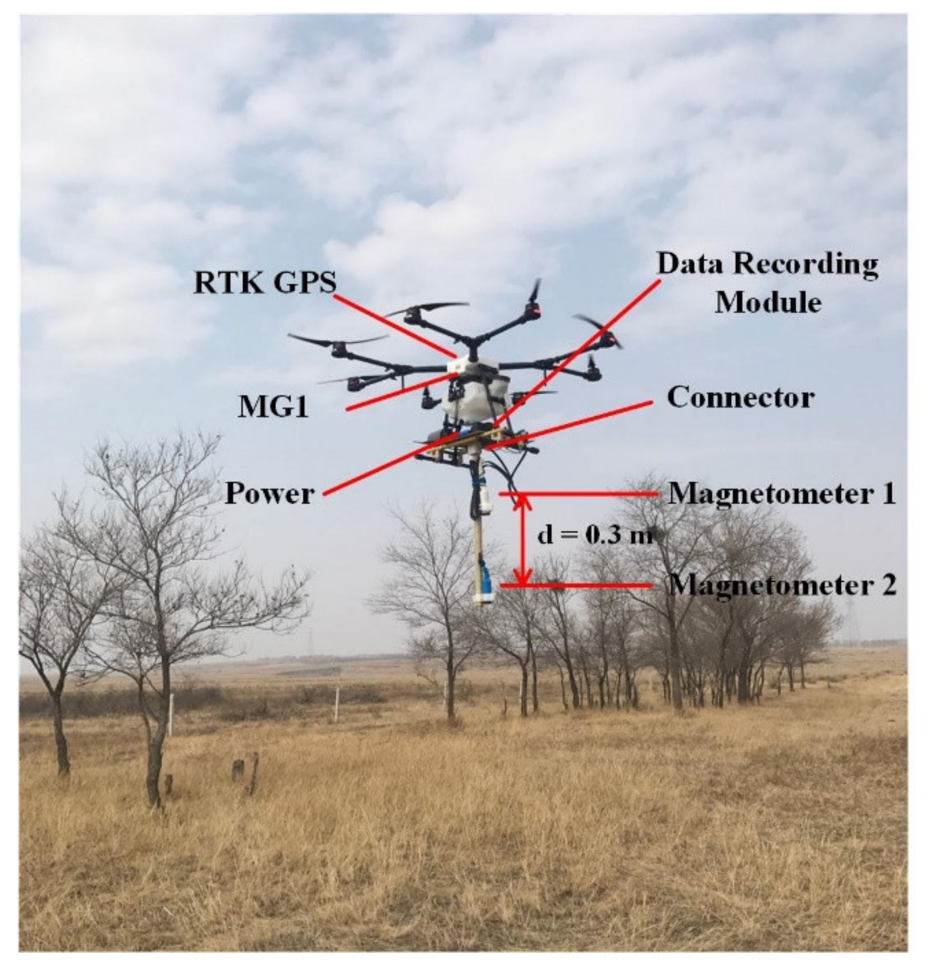
Figure 5a,b demonstrate the measured results of magnetometer 1 and magnetometer 2, low-pass filtering and DC removal have been executed, and the extracted magnetic anomaly field after removing the UAV interference field is shown in Figure 5c.
Magnetometer 1 is closer to the drone than magnetometer 2, and the interference field measured by magnetometer 1 is larger, the root mean square (rms) errors of the two measured magnetic signals are 5.485 nT and 2.663 nT. The magnetic anomaly signal is separated from the measured results according to the method in Supplementary Materials, the platform interference magnetic field is significantly reduced, rms is reduced to 1.077 nT.

3.2. The Inversion of Magnetic Field

For the ferromagnetic target in the shallow subsurface, when the distance between the sensor and the target is more than three times the maximum size of the target, the induced magnetic field generated by the target can be approximated as a point-shaped magnetic dipole. The dipole model is a point model, ignoring the shape and posture information of the target, and it can be characterized by six parameters including three-dimensional position vector and three-dimensional magnetic moment vector. The position vector provides the information about the location of the target, and the magnetic moment vector is related to the posture, shape, and material of the target.
A magnetic dipole is located at r 0 = r 0 x , r 0 y , r 0 z , the magnetic moment is m = m x ,   m y ,   m z , and the magnetic field B d i p o l e at the observation point r p is:
B d i p o l e r , m = µ 0 4 π 3 m r r r 5 m r 3
µ 0 is the permeability in the vacuum, and equals to 4 π × 10 7 H/m, r is the distance vector from the observation point r p to the dipole r 0 , and r is its modulus.
Assuming that there is no measurement noise, the output of the optically pumped magnetometer B t o t a l is the superposition of the geomagnetic field and the projection of the induced magnetic field in the direction of the geomagnetic field [31]:
B t o t a l = B e a r t h + B d i p o l e · B e a r t h B e a r t h
B e a r t h is the geomagnetic field, B e a r t h is its magnitude.
Consequently, the magnetic anomaly field Δ T is related to the magnetic moment and position of the dipole, written as:
Δ T = f r , m = B d i p o l e · B e a r t h B e a r t h
The inversion problem is to invert the position r 0 and magnetic moment m based on the magnetic anomaly signal ( Δ T i , i = 1, 2, …, N) at multiple observation points ( r p , i = 1, 2, …, N), six unknown parameters form the feature vector x = r 0 x , r 0 y , r 0 z , m x , m y , m z . The differential evolution (DE) algorithm is adopted to estimate x, which is a classic heuristic random search algorithm [32,33]. DE is a global optimization strategy, suitable for solving noisy, multi-objective optimization problem.
The objective function is established by minimizing the data misfit between predicted magnetic anomaly field and observed magnetic anomaly field Δ T i . The predicted magnetic anomaly field f i x of the ferromagnetic target is based on Equation (3), so the objection function is expressed as follows:
arg min x i = 1 N f i x Δ T i 2
The inversion flow of magnetic data is listed in Algorithm 1. The feature vector x inverted from the magnetic data provides the position and magnetic moment of the buried target.
Algorithm 1. The Inversion of Magnetic Field.
Input: Magnetic anomaly field Δ T i ; The range of feature vector: x min j , x max j (j = 1,2,..,6)
Population: M; Dimension: D; Generation: T
Output: The location and magnetic moment vector of the target: x ^
1  t 1 (Initialization);
2  for i = 1 to M do
3 for j = 1 to D do
4   x i , t j = x min j + r a n d 0 , 1 x max j x min j ;
5 end
6  end
7  while  t T  or  f x ^ ε  do
8 for i = 1 to M do
9  for j = 1 to D do
10    v i , t j = M u t a t i o n x i , t j ;
11    u i , t j = C r o s s o v e r x i , t j , v i , t j ;
12  end
13  if  f u i , t < f x i , t then
14    x i , t u i , t ;
15   if  f x i , t < f x ^ then
16     x ^ x i , t ;
17   end
18  else
19    x i , t x i , t ;
20  end
21 end
22 t t + 1;
23  end
24  return feature vector x ^ including location and magnetic moment

3.3. EM Data Processing

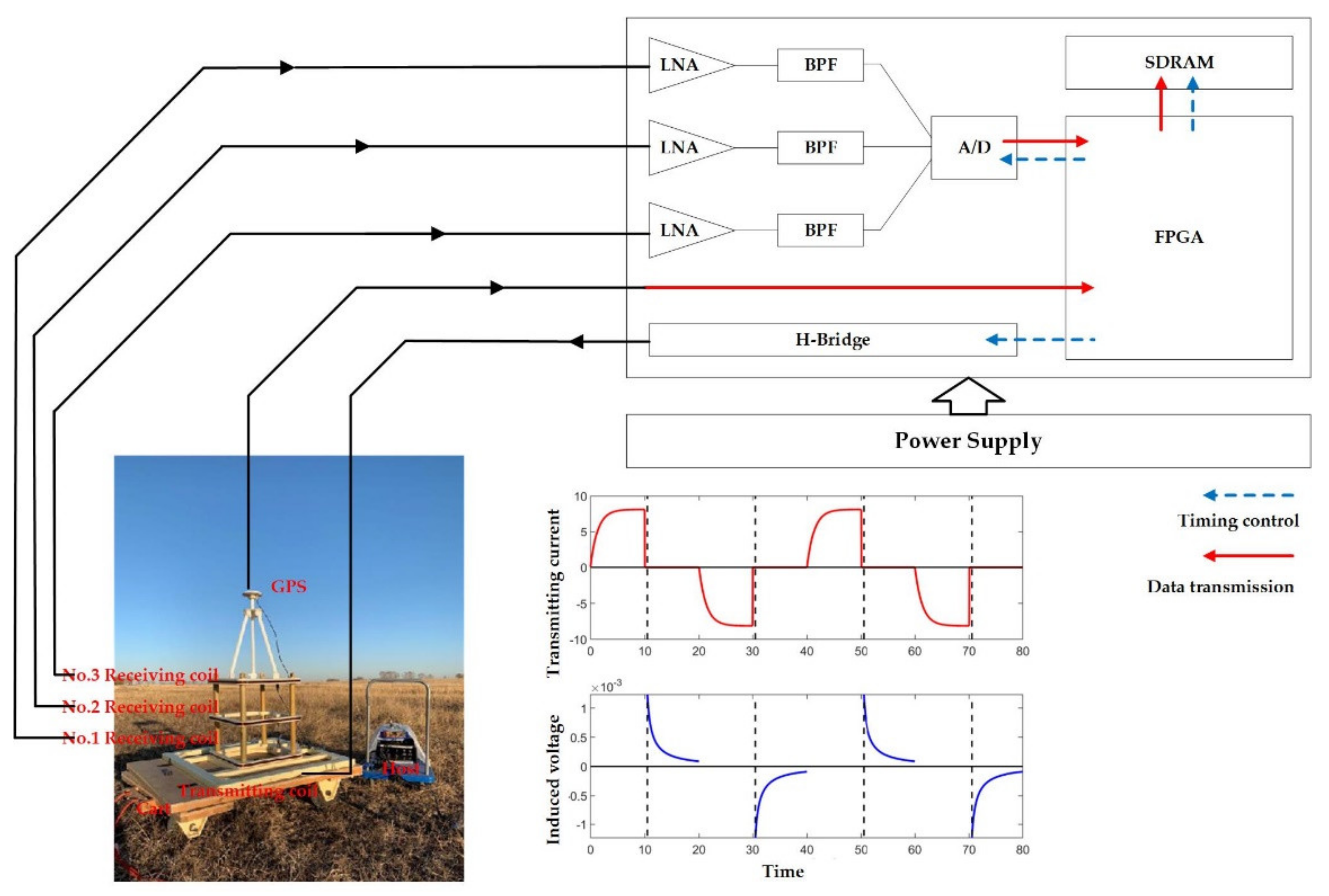
TDEM-Cart system receives the secondary field generated by the target and converts it into the voltage signal through the induction coil. Its working principle is Faraday’s law of induction, and the working frequency band is very wide. The electromagnetic noise in the ambient environment is overlapped with the response of the target, the SNR of the secondary field will be reduced, degrading the detection performance. Therefore, some signal processing methods are utilized to eliminate the environmental noise and improve the SNR.

3.3.1. Signal Stacking

The emission current of the TDEM-Cart is a bipolar square wave, so the corresponding secondary field is also alternately positive and negative. Assuming that the received data has n ( n 1 ) periods, there are a total of 2n positive and negative response signals. The negative polarity response is reversed and superimposed with the positive polarity response:
V s t = V i t s n t
V i t and V s t are the signals before and after stacking, and s n t is the stacking function, expressed as:
s n t = 1 2 n δ t δ t T 2 + δ t T + 1 2 n 1 δ t 2 n 1 T 2 = 1 2 n m = 0 2 n 1 1 m δ t m T 2
n denotes the number of the stacking period, T is the period of the emission current, δ t is the Dirichlet function.
To understand the Equations (5) and (6), the Fourier functions of the two stacking functions with n = 1 and n = 8 are demonstrated in Figure 6a. It shows that the stacking procedure eventually renders a narrow-band, match-filter-type band pass filter in time domain, and the larger the number of periods n, the narrower the bandwidth of the filter. Figure 6b demonstrates the same result in time domain, three response signals with different stacking cycle n = 0, 1, 8 are compared. As the number of superimposed cycles increases, the noise suppression is enhanced, especially in the late stage of the signal.

3.3.2. Windowing in Time Domain

In time domain, multiple time windows distributed at equal intervals are designed, and the integrated average value of the received signal in each time window is calculated to obtain the final response curve. The induced voltage after windowing procedure in time domain is obtained:
V w t = V s t w n t t n d t
V s t denotes the induced voltage signal after stacking, V w t denotes the voltage signal after windowing, t n is the center of the window function, w n t is the rectangular window function, written as:
w n t = 1 T n t T n 2 0 t > T n 2
where T n is the length of the rectangular window. Analyzed in frequency domain, the Fourier function of the rectangular window is equivalent to a low-pass filter, so the windowing process can eliminate out-of-band noise. Figure 7 shows the comparison of received voltage signals before and after windowing, indicating that the late SNR of the response signal has been improved a lot through the time window processing.

3.4. The Inversion of EM Data

Similar to the inversion of magnetic field data, the secondary field generated by the target is approximated by a three-dimensional magnetic dipole for the long-distance detection system. The difference is, the magnetic moment of the dipole is a constant in the inversion of magnetic data, while the magnetic moment of the dipole in EM detection is a time-dependent parameter, because the primary field is time-varying.
According to the theory proposed by L. R. Pasion [23,34], the magnetic moment m E M t has the form:
m E M t = 2 π µ 0 A T F E M t A b E M P = h E M φ , θ , L 1 ( t ) , L 2 ( t ) , L 3 ( t )
where A is the Euler rotation tensor, determined by the azimuth φ and dip θ that are the rotation angle and the inclination angle between the local coordinate system where the target is located and the global coordinate system. b E M P is the primary field at the location of the target, F E M t is the electromagnetic polarization tensor, characterized by three diagonal elements L 1 t , L 2 t , L 3 t , L i t (i = 1,2,3) denotes the intrinsic response of the 3D magnetic dipole along the i-th direction, and L i t is estimated as [34]:
L i t = k i t β i exp t / γ i
where k i is the magnitude of the polarization, β i defines the power law decay, γ i 
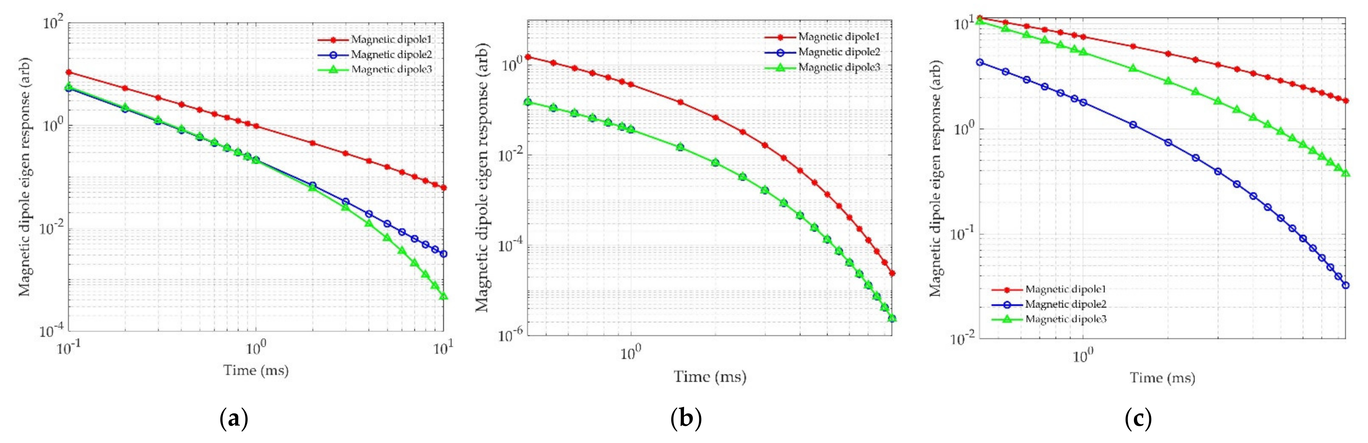
is the fundamental time constant. Once the three parameters k i , β i , γ i are determined, the intrinsic response curve of the magnetic dipole versus time can be estimated.
Combined (9) and (10), the function h E M () is a unified representation for Equations (9) and (10), so the magnetic moment of dipole is described as:
m E M t = h E M φ , θ , k 1 , β 1 , γ 1 , k 2 , β 2 , γ 2 , k 3 , β 3 , γ 3
Based on the hypothesis of magnetic dipole, the EM feature vector y contains 14 unknown parameters, including 3 position parameters related to the location of target, 2 angle parameters related to posture of target and 9 parameters related to shape characteristics of target:
y = x 0 , y 0 , z 0 , φ , θ , k 1 , β 1 , γ 1 , k 2 , β 2 , γ 2 , k 3 , β 3 , γ 3
The objective function of the electromagnetic inversion is established to minimize the misfit between the received voltage signal d o b s i and the predicted the dipole response g i y . The function g i () in (13) is a unified representation for calculating the magnetic field generated by a dipole in Equation (1), the objective function of EM inversion is derived as follows:
arg min y i = 1 N g i y d o b s i 2
Levenberg–Marquardt (LM) algorithm is adopted to invert the feature vector y, which is a trust region method for solving the nonlinear problem [35]. LM is a local optimization strategy with the advantage of fast convergence.
Figure 8 is the flow chart of the joint inversion. It is worth emphasizing that the inversion results of the magnetic field is set as the initial value of the EM inversion, providing a priori information about the target location. The joint inversion method belongs to the “feature level” sensor fusion [27], the inversion result of the joint magnetic field and electromagnetic data is a fused feature vector, containing a three-dimensional position and two attitude angles of the target, and the shape feature of the target can be inferred from the intrinsic response curve of the magnetic dipole, realizing the classification of the target.

4. Experiments and Results

We have conducted two field tests to evaluate the performance of the joint detection system, and performed the cooperative inversion of the magnetic and electromagnetic data. In the first experiment, the joint detection system worked in full coverage survey mode. Both UAVMAG and TDEM-Cart were employed to survey the whole test area, and the mapping result of magnetic field data and electromagnetic data were compared. In the second experiment, the joint detection system worked in the cued survey mode. The whole test area was surveyed by the UAVMAG firstly. Then, a series of small-area fine surveys in the vicinity of the targets were carried out by the TDEM-Cart system, the cooperative inversion has been applied for the location and recognition of target.

4.1. Full Coverage Survey

4.1.1. Experimental Setup

This experiment was conducted in a suburb, Hebei Province, China. Three metal targets were pre-buried into the test area, as shown in Figure 9a. Among them, 1# and 2# targets are made of iron, 3# target is an aluminum triangle target.
The joint detection system worked in the full coverage survey mode. Firstly, the magnetic data was collected by the UAVMAG. The flight profiles have been planned in advance, the profiles are along the north–south direction, the height above the ground is 2 m, the interval is approximately 0.5 m, the error is less than 0.2 m affected by the weather. There are a total of 40 lateral lines, covering the entire test area. Then, the EM data was collected by the TDEM-cart system, and 9 lines with spacing 1 m were planned to cover the entire test area. Figure 9b,c show the actual UAVMAG flight trajectory and TDEM-cart test trajectory, the turning tracks are cut, leaving only the parallel profiles.
The magnetic data and EM data have been collected by the UAVMAG and TDEM-Cart system. Two data sets are synchronized based on the spatial location information measured by RTK GPS, and the positioning error is at the centimeter level. A unified cartesian coordinate system is established, and the origin is the take-off point of the drone, the x-axis points to the east, the y-axis points to the north, the z-axis points to up.

4.1.2. Results

The raw magnetic data measured by the magnetometer 1 and magnetometer 2 are given in Figure 10a,b, the magnetic anomaly field is extracted from the total magnetic field by the signal processing methods in Section 3.1, and Figure 10c demonstrates the mapping result of the magnetic anomaly signal over the entire test area. Compared with the magnetic map of raw data, the SNR of the processed signal has been improved a lot. Two magnetic anomalies are clearly observed from Figure 10c, which are in line with the preset positions of the 1# and 2# targets, whereas 3# target made of aluminum cannot be detected from the mapping result of magnetic data. The experimental results are consistent with the theoretical analysis, UAVMAG can only detect targets with high permeability.
The electromagnetic signal received by the TDEM-cart system decays with time. In order to map the secondary field, we obtained the spatial distribution of the voltage signal at the receiver through stacking and windowing methods described in Section 3.3. Figure 11a,b are the map of the response signal measured by No.1 receiving coil at t = 0.67 ms and t = 4.5 ms. Both early and late response signals show that there are three obvious abnormal signals in the test area, indicating that three metal targets may be buried. Furthermore, the spatial location of the abnormal signal is in agreement with the position of pre-buried targets. It is worth noting that the 3# target can be detected by the TDEM-Cart system, avoiding missed detection.
Therefore, when the joint detection system works in the full coverage survey mode, the combination of magnetic and electromagnetic signal is able to improve the reliability of the detection results and avoid missed inspections.

4.2. Cued Survey

4.2.1. Experimental Setup

This experiment was also conducted in a suburb, Hebei Province, China. Three ferromagnetic targets were pre-buried into the test area, marked as the 4#, 5#, and 6# target as shown in Figure 12. The responses of 4# target and 5# target are similar to UXO, which are used to simulate the real UXO, and 6# target is used to simulate the clutter. 4# target was buried at an angle of 45 degrees in the north–south direction, 5# and 6# targets were buried vertically, the location of the three targets were measured by the RTK GPS in advance. The position, azimuth and dip, shape feature of three targets are given in Table 1.
The joint detection system worked in the cued survey mode, a unified coordinate system was established, realizing the synchronization of magnetic and electromagnetic data in space.

4.2.2. Results

Firstly, the raw magnetic data was collected by the UAVMAG, and signal processing methods in Section 3.1 have been executed to extract the magnetic anomaly field related to the target. Figure 13a displays the magnetic anomaly field over the entire test area. The magnetic anomaly field generated by an isolated target is bipolar, including a positive anomaly field and a negative anomaly field. Three targets in the test area are observed from the mapping result. The magnetic anomaly signal produced by a single target has been manually separated, as shown in Figure 13b,d. Then, the DE algorithm proposed in Section 3.2 is employed to invert the feature vector x, and R-squared (R2) is used to measure the convergence of the inversion model. The position and magnetic moment of the three targets and model fit are listed in Table 2.
Next, potential targets have been delineated in the test area according to feature vector x. TDEM-Cart system was used to carry out finer surveys over the local areas near the targets. Three maps of received voltage at t = 0.67 ms are depicted in Figure 14.
Finally, EM inversion is performed based on electromagnetic data in three local areas, the initial value of EM inversion is set according to the feature vector x, the feature vector y of three targets retrieved from EM data and model fit are given in Table 3, and the magnetic dipole eigen responses of three targets are demonstrated in Figure 15.
The feature vector x inverted from the magnetic data only provides the position and magnetic moment of ferrous targets, the posture, shape cannot be estimated. Comparing the position parameters in Table 1 and Table 2, the positioning error of the individual inversion of magnetic data is evaluated. The minimum positioning error in X is 0.04 m, the maximum is 0.26 m; the minimum positioning error in Y is 0.11 m, the maximum is 0.34 m; the minimum positioning error in Z is 0.04 m, the maximum is 0.07 m. In addition, based on the empirical analysis, it can be considered that the 3# target with the smallest magnetic moment might be a smaller target, which is consistent with the actual situation. However, the size of 1# and 2# target cannot be judged from the inverted magnetic moment.
The feature vector y derived from combined magnetic and EM data provides more information, including the position of the target, the azimuth and dip, and the magnetic dipole eigen response. Comparing the position parameters in Table 1 and Table 3, the positioning error of joint inversion in X, Y, and Z are all less than 0.1 m, verifying that the positioning accuracy estimated by the joint inversion is higher than that of individual inversion technique.
Comparing the angle parameters in Table 1 and Table 3, the inverted the attitude angle of the 4# and 5# targets are more accurate, error is less than 10°, whereas the calculation error of the 6# target is slightly larger. The reason is related to the assumption of the dipole model in the inversion theory, it’s difficult to use merely azimuth and dip to characterize its posture information for the irregularly shaped target.
Based on the dipole eigen response curve in Figure 15, the intrinsic responses of 4# target and 5# target have similar characteristics that the dipole response along the long principal axis is much larger than the dipole response in the other two directions, and decays more slowly over time, the dipole intrinsic curves in the direction of the two short principal axis basically coincide, indicating that 4# and 5# target may be rod-like and axisymmetric, which are in agreement with the characteristics of UXO. The intrinsic responses of 6# target in the three directions also attenuate with time, but its attenuation curves and amplitude are completely different, which conforms to the characteristics of irregularly shaped clutter.

5. Discussion

This paper introduces the joint remote detection system, which combines the UAV magnetic survey (UAVMAG) and the vehicle-mounted time domain electromagnetic system (TDEM-Cart), and the cooperative processing flow is designed, fusing the feature vectors inverted from magnetic data and electromagnetic data. Compared with the single detection technology [4,5,6,7,8,9], existing airborne and ground-based joint detection modes [24,25,26], the combination method proposed in this paper has significant advantages in terms of positioning accuracy and detection efficiency.
Compared with the individual magnetic detection, the joint detection system is capable of detecting both ferromagnetic and non-ferromagnetic metal targets, overcoming the shortcomings that only ferrous targets can be detected by the magnetic survey. In the first experiment, the joint detection system worked in full-coverage survey mode, and the experimental results confirm that the joint detection system is able to detect the target made of aluminum.
Compared with the single electromagnetic method, the joint detection system can improve the detection efficiency. When the joint detection system works in the cued survey mode, the rapid and complete scanning detection is firstly conducted by the UAVMAG, and potential abnormal regions are delineated according to the result of magnetic survey. Then, local fine surveys in the vicinity of the targets are performed by TDEM-Cart system, avoiding covering the entire test area and greatly shortening the working time.
For the cooperative interpretation, the inversion of magnetic data is based on the global optimization algorithm DE, the inversion of EM data fuses the feature vector inverted from magnetic data and adopts the local optimization algorithm LM. The proposed joint inversion process can not only improve the positioning result of the target, but also avoid falling into the local optimal solution. In the second experiment, the maximum positioning error of the magnetic field inversion reaches 34 cm, and the target positioning deviation after the joint inversion is less than 10 cm. In addition, the posture and shape characteristics of the target are inferred based on the two attitude angles and dipole intrinsic response over time, which are basically in line with the characteristics of the actual buried targets. The experimental results indicate that the accuracy of cooperative interpretation is higher, which is of great significance to the classification and recognition of targets. Nonetheless, it should be noted that the proposed joint processing algorithm is only suitable for the inversion of an isolated target.
Compared with the joint detection system in [23] with the combination of handheld magnetic survey and ground-based TDEM, the combined detection method proposed in this paper has higher detection efficiency than the ground magnetic survey, which is more suitable for large-scale survey and rapid monitoring. In [18], the UAV-mounted TDEM system has been developed, and the field experiments were carried out to detect UXO. The combination of the UAV-borne magnetic detection system and the UAV-borne electromagnetic system is bound to have better performance, which is the focus of future research.

6. Conclusions

In this paper, we concentrated on the remote detection of near-surface targets and interested in estimating the position, shape, and attitude information of the target. The main contents could be concluded that:
(1)
The joint detection system has been developed, including the drone-based magnetic detection system UAVMAG and the vehicle-mounted time domain electromagnetic detection system TDEM-Cart. The magnetic field data and electromagnetic data are synchronized through the spatial position measured by RTK GPS.
(2)
The processing flow consists of four parts, magnetic field signal processing, the inversion of magnetic data, EM data processing, and the inversion of EM data. The electromagnetic data inversion in the fourth step depends on the feature vector obtained from the inversion results in the second step, which belongs to the “feature level” sensor fusion.
(3)
In the first field test, the joint detection system worked in the full-coverage survey mode, both ferromagnetic and non-ferromagnetic metal targets can be detected.
(4)
In the second field test, the joint detection system worked in the cued survey mode, the position, shape, and attitude information of the target are derived based on the cooperative processing methods. The positioning accuracy is less than 10 cm and shows satisfactory performance in the recognition of target.

Supplementary Materials

The elimination of UAV interference field in Section 3.1.3 can refer to our paper, available online at: https://www.mdpi.com/article/10.3390/rs13122343/s1.

Author Contributions

Y.M. and W.X. proposed the methodology; Y.M., W.X. and X.Z. designed the validation scheme; Y.M. and W.X. performed the field tests; Y.M. and W.X analyzed the data; Y.M wrote the paper. All authors have read and agreed to the published version of the manuscript.

Funding

The research was funded by the research project “National Natural Science Foundation of China”, which is supported by the Chinese government, grant number is 41604155.

Institutional Review Board Statement

Not applicable.

Informed Consent Statement

Not applicable.

Data Availability Statement

Not applicable.

Acknowledgments

The authors would like to thank the associate editor and anonymous reviewers for their valuable comments that helped to correct and improve the clarity of this letter.

Conflicts of Interest

The authors declare no conflict of interest.

References

  1. Butler, D.K. What is near-surface geophysics? In Near-Surface Geophysics, 2nd ed.; Butler, D.K., Ed.; Society of Exploration Geophysicists: Tulsa, OK, USA, 2005; Volume 3, pp. 1–6. [Google Scholar]
  2. Qu, X.; Wang, C.; Fang, G.; Yin, H. Detecting anomaly targets using handheld frequency domain electromagnetic system. Sens. Actuator A Phys. 2017, 268, 155–163. [Google Scholar]
  3. Nelson, H.H.; McDonald, J.R. Multisensor towed array detection system for UXO detection. IEEE Trans. Geosci. Remote Sens. 2001, 390, 1139–1145. [Google Scholar] [CrossRef] [Green Version]
  4. Munschy, M.; Boulanger, D.; Ulrich, P.; Bouiflane, M. Magnetic mapping for the detection and characterization of UXO: Use of multi-sensor fluxgate 3-axis magnetometers and methods of interpretation. J. Appl. Geophys. 2007, 61, 168–183. [Google Scholar] [CrossRef]
  5. Billings, S.; Wright, D. Interpretation of high-resolution low-altitude helicopter magnetometer surveys over sites contaminated with unexploded ordnance. J. Appl. Geophys. 2010, 72, 225–231. [Google Scholar] [CrossRef]
  6. Butler, D.K.; Simms, J.E.; Furey, J.S.; Bennett, H.H. Review of magnetic modeling for UXO and applications to small items and close distances. J. Environ. Eng. Geophys. 2012, 17, 53–73. [Google Scholar] [CrossRef]
  7. EM61-MK2. Available online: http://www.geonics.com/html/em61-mk2.html (accessed on 25 April 2021).
  8. EM63-3D-MK2. Available online: http://www.geonics.com/html/metaldetectors.html (accessed on 25 April 2021).
  9. Daniels, D.J. A review of GPR for landmine detection. Sens. Imaging 2006, 7, 90–123. [Google Scholar] [CrossRef]
  10. Takahashi, K.; Igel, J.; Preetz, H.; Sato, M. Influence of heterogeneous soils and clutter on the performance of ground-penetrating radar for landmine detection. IEEE Trans. Geosci. Remote Sens. 2014, 52, 3464–3472. [Google Scholar] [CrossRef]
  11. Wiegert, R.; Lee, K.; Oeschger, J. Improved magnetic STAR methods for real-time, point-by-point localization of unexploded ordnance and buried mines. In Proceedings of the OCEANS 2008, Kobe, Japan, 8–11 April 2008. [Google Scholar]
  12. Stolz, R.; Schmelz, M.; Zakosarenko2, V.; Foley, C.; Tanabe, K.; Xie, X.; Fagaly, R.L. Superconducting sensors and methods in geophysical applications. Supercond. Sci. Technol. 2021, 34. [Google Scholar]
  13. Gavazzi, B.; Le Maire, P.; Munschy, M.; Dechamp, A. Fluxgate vector magnetometers: A multisensor device for ground, UAV, and airborne magnetic surveys. Lead. Edge 2016, 35, 795–797. [Google Scholar] [CrossRef] [Green Version]
  14. Mu, Y.; Zhang, X.; Xie, W.; Zheng, Y. Automatic detection of near-surface targets for Unmanned Aerial Vehicle (UAV) magnetic survey. Remote Sens. 2020, 12, 452. [Google Scholar] [CrossRef] [Green Version]
  15. Døssing, A.; Silva, E.L.S.; Martelet, G.; Rasmussen, T.M.; Gloaguen, E.; Petersen, J.T.; Linde, J. A high-seed, light-weight scalar magnetometer bird for km scale UAV magnetic surveying: On sensor choice, bird design, and quality of output data. Remote Sens. 2021, 13, 649. [Google Scholar] [CrossRef]
  16. Malehmir, A.; Dynesius, L.; Paulusson, K.; Paulusson, A.; Johansson, H.; Bastani, M.; Wedmark, M.; Marsden, P. The potential of rotary-wing UAV-based magnetic surveys for mineral exploration: A case study from central Sweden. Lead. Edge 2017, 36, 552–557. [Google Scholar] [CrossRef]
  17. Fernández, J.P.; Barrowes, B.; Bijamov, A.; Grzegorczyk, T.; Lhomme, N.; O’Neill, K.; Shamatava, I.; Shubitidze, F. MPV-II: An enhanced vector man-portable EMI sensor for UXO identification. In Proceedings of the SPIE 8017, Detection and Sensing of Mines, Explosive Objects, and Obscured Targets XVI, Orlando, FL, USA, 23 May 2011. [Google Scholar]
  18. Qi, Z.; Li, X.; Li, H.; Liu, W. First results from drone-based transient electromagnetic survey to map and detect unexploded ordnance. IEEE Geosci. Remote Sens. Lett. 2020, 17, 2055–2059. [Google Scholar] [CrossRef]
  19. Ralchenko, M.; Samson, C.; Holladay, S.; Polowick, C. Towards an unmanned airborne platform for electromagnetic geophysical surveying. In Proceedings of the 2018 SEG International Exposition and Annual Meeting, Anaheim, CA, USA, 14–19 October 2018. [Google Scholar]
  20. Parshin, A.; Bashkeev, A.; Davidenko, Y.; Persova, M.; Iakovlev, S.; Bukhalov, S.; Grebenkin, N.; Tokareva, M. Lightweight unmanned aerial system for time-domain electromagnetic prospecting—the next stage in applied UAV-Geophysics. Appl. Sci. 2021, 11, 2060. [Google Scholar] [CrossRef]
  21. Bjerg, T.; Lima, E.; Silva, S.; Døssing, A. Investigation of UAV noise reduction for electromagnetic induction surveying. In Proceedings of the NSG2020 3rd Conference on Geophysics for Mineral Exploration and Mining, Online, 7–8 December 2020. [Google Scholar]
  22. Xie, W.; Zhang, X.; Mu, Y.; Zheng, Y. A subsurface targets’ classification method utilizing gradient learning technique. IEEE Geosci. Remote Sens. Lett. 2020. [Google Scholar] [CrossRef]
  23. Pasion, L.R.; Billings, S.D.; Kingdon, K.A.; Oldenburg, D.W.; Lhomme, N.; Jacobson, J. Cooperative inversion of time domain electromagnetic and magnetometer data for the discrimination of unexploded ordnance. J. Environ. Eng. Geophys 2008, 13, 193–210. [Google Scholar] [CrossRef]
  24. Young, R.; Siegel, R.; Crandall, A. Combined Electromagnetic and Magnetometer Data Acquisition and Processing; Environmental Security Technology Certification Program: Alexandria, VA, USA, 2005. [Google Scholar]
  25. Sheehan, J.; Beard, L.; Gamey, J.; Doll, W.; Norton, J. UXO detection and prioritization using combined airborne vertical magnetic gradient and time-domain electromagnetic methods. In Proceedings of the 2008 SEG Annual Meeting, Las Vegas, NV, USA, 9–14 November 2008. [Google Scholar]
  26. Okazaki, K.; Mogi, T.; Utsugi, M.; Ito, Y.; Kunishima, H.; Yamazaki, T.; Takahashi, Y.; Hashimoto, T.; Ymamaya, Y.; Ito, H.; et al. Airborne electromagnetic and magnetic surveys for long tunnel construction design. Phys. Chem. Earth 2011, 36, 1237–1246. [Google Scholar] [CrossRef]
  27. Gravina, R.; Alinia, P.; Ghasemzadeh, H.; Fortino, G. Multi-sensor fusion in body sensor networks: State-of-the-art and research challenges. Inf. Fusion 2017, 35, 68–80. [Google Scholar] [CrossRef]
  28. Niu, X.; Yan, K.; Zhang, T.; Zhang, Q.; Zhang, H.; Liu, J. Quality evaluation of the pulse per second (PPS) signals from commercial GNSS receivers. GPS Solut. 2015, 19, 141–150. [Google Scholar] [CrossRef]
  29. Hansen, R.O.; Racic, L.; Grauch, V.J.S. Magnetic methods in near-surface geophysics. In Near-Surface Geophysics, 2nd ed.; Butler, D.K., Ed.; Society of Exploration Geophysicists: Tulsa, OK, USA, 2005; pp. 151–175. [Google Scholar]
  30. Daya, Z.A.; Birsan, M.; Holtham, P.M.; Holtham, P.M. The magnitude and distribution of ambient fluctuations in the scalar magnetic field. In Proceedings of the OCEANS 2005 MTS, Washington, DC, USA, 17–23 September 2005; IEEE: Piscataway, NJ, USA, 2005. [Google Scholar]
  31. Sheinker, A.; Shkalim, A.; Salomonski, N.; Ginzburg, B.; Frumkis, L.; Kaplan, B. Processing of a scalar magnetometer signal contaminated by 1/fα noise. Sens. Actuator A Phys. 2007, 138, 105–111. [Google Scholar] [CrossRef]
  32. Storn, R.; Price, K.V. Differential evolution—a simple and efficient heuristic for global optimization over continuous spaces. J. Glob. Optim. 1997, 11, 341–359. [Google Scholar] [CrossRef]
  33. Das, S.; Suganthan, P.N. Differential evolution: A survey of the state-of-the-art. IEEE Trans. Evol. Comput. 2011, 15, 4–31. [Google Scholar] [CrossRef]
  34. Pasion, L.R. The Inversion of Time Domain Electromagnetic Data for the Detection of Unexploded Ordnance. Ph.D. Thesis, University of British Columbia, Vancouver, BC, Canada, 2007. [Google Scholar]
  35. Pujol, J. The solution of nonlinear inverse problems and the Levenberg-Marquardt method. Geophysics 2007, 72, W1–W16. [Google Scholar] [CrossRef]
Figure 1. The UAVMAG system, the vertical distance between two magnetometers is 0.3 m.
Remotesensing 13 02343 g001
Figure 2. TDEM-cart system and the basic electronic block diagram. The schematic diagrams of the emission current and the receiving voltage are also illustrated.
Remotesensing 13 02343 g002
Figure 3. The frequency spectrum before (blue) and after (red) the lowpass filtering.
Remotesensing 13 02343 g003
Figure 4. The elimination of the geomagnetic field. (a) Filtered magnetic field data before removing the DC component. (b) The magnetic field data after removing the DC component.
Remotesensing 13 02343 g004
Figure 5. The elimination of the UAV interference field. (a) The measured magnetic field by the magnetometer 1. (b) The measured magnetic field by the magnetometer 2. (c) The extracted magnetic anomaly field.
Remotesensing 13 02343 g005
Figure 6. The stacking operation. (a) The spectrum of stacking function (n = 1, 8). (b) The response signal with different stacking cycle (n = 0, 1, 8).
Remotesensing 13 02343 g006
Figure 7. The comparison of response before (blue) and after (red) time window processing.
Remotesensing 13 02343 g007
Figure 8. Flow chart of joint inversion of magnetic data and EM data.
Remotesensing 13 02343 g008
Figure 9. The graph of targets and profiles, the red symbol ‘*’ indicates the location of the target measured by RTK GPS. (a) Three targets to be tested. (b) The flight path of UVAMAG. (c) The lines measured by TDEM-Cart.
Remotesensing 13 02343 g009
Figure 10. The magnetic map measured by UAVMAG; the unit of magnetic field is nano Tesla (nT). (a) The magnetic map of raw data measured by magnetometer 1. (b) The magnetic map of raw data measured by magnetometer 2. (c) The magnetic map of magnetic anomaly field processed by the methods in Section 3.1.
Remotesensing 13 02343 g010
Figure 11. The induced voltage signal map measured by the No.1 receiving coil of TDEM-Cart; the unit is mV. (a) The response signal map at t = 0.67 ms. (b) The response signal map at t = 4.5 ms.
Remotesensing 13 02343 g011
Figure 12. The targets to be tested in the second experiment.
Remotesensing 13 02343 g012
Figure 13. The map of magnetic anomaly field, the unit of magnetic field is nT. (a) The magnetic anomaly field over the entire survey area. (b) Magnetic anomaly field generated by 4# target. (c) Magnetic anomaly field generated by 5# target. (d) Magnetic anomaly field generated by 6# target.
Remotesensing 13 02343 g013
Figure 14. Three maps of received voltage by TEDM-Cart at t = 0.67 ms, the unit is mV. (a) The induced voltage generated by 4# target. (b) The induced voltage generated by 5# target. (c) The induced voltage generated by 6# target.
Remotesensing 13 02343 g014
Figure 15. The magnetic dipole eigen response over time. (a) 4# target. (b) 5# target. (c) 6# target.
Remotesensing 13 02343 g015
Table 1. The basic parameters of three targets.
4# Target5# Target6# Target
Location (m)(6.17,33.96,−0.8)(6.31,26.61,−1.0)(3.99,22.15,−0.1)
Attitude angle
φ , θ
0 ° , 45 ° 0 ° , 0 ° 0 ° , 0 °
Shape featurerod-likerod-likeIrregualr-shape
Table 2. The inversion results from magnetic data.
4# Target5# Target6# Target
Location (m)(5.91,34.07,−0.86)(6.35,26.41,−1.07)(3.85,21.81,−0.06)
Magnetic moment
(Am2)
(−0.016,2.14,−2.39)(−0.194,−2.21,2.54)(−0.001,−0.4,−0.05)
Model fit90.81%94.79%86.18%
Table 3. The inversion results from EM data.
4# Target5# Target6# Target
Location (m)(6.11,34.00,−0.83)(6.31,26.55,−1.03)(3.89,22.08,−0.08)
Attitude angle
φ , θ
0 ° , 40.21 ° 0 ° , 9.86 ° 8.53 ° , 12.88 °
Model fit 91.79%93.90%96.82%
Publisher’s Note: MDPI stays neutral with regard to jurisdictional claims in published maps and institutional affiliations.

