Article

Evaluating Short-Term Tidal Flat Evolution Through UAV Surveys: A Case Study in the Po Delta (Italy)

Department of Physics and Earth Sciences, University of Ferrara, 44122 Ferrara, Italy
*
Author to whom correspondence should be addressed.
Remote Sens. 2021, 13(12), 2322; https://doi.org/10.3390/rs13122322
Submission received: 31 March 2021 / Revised: 10 June 2021 / Accepted: 10 June 2021 / Published: 13 June 2021
(This article belongs to the Special Issue UAV Application for Monitoring Coastal Morphology)

Abstract

:
The use of Unmanned Aerial Vehicles (UAV) on wetlands is becoming a common survey technique that is extremely useful for understanding tidal flats and salt marshes. However, its implementation is not straightforward because of the complexity of the environment and fieldwork conditions. This paper presents the morphological evolution of the Po della Pila tidal flat in the municipality of Porto Tolle (Italy) and discusses the reliability of UAV-derived Digital Surface Models (DSMs) for such environments. Four UAV surveys were performed between October 2018 and February 2020 on an 8 ha young tidal flat that was generated, amongst others, as a consequence of the massive sediment injection into the Po Delta system due to the floods of the 1950s and 1960s. The DSM accuracy was tested by processing (i.e., photogrammetry) diverse sets of pictures taken at different altitudes during the same survey day. The DSMs and the orthophotos show that the tidal flat is characterised by several crevasse splays and that the sediment provision depends strictly on the river. During the study period, the sediment budget was positive (gaining 800 m3/year and an average rate of vertical changes of 1.3 cm/year). Comparisons of DSMs demonstrated that neither lower flight altitudes (i.e., 20–100 m) nor the combination of more photos from different flights during the same surveys necessarily reduce the error in such environments. However, centimetric errors (i.e., RMSEs) are achievable flying at 80–100 m, as the increase of GCP (Ground Control Point) density is the most effective solution for enhancing the resolution. Guidelines are suggested for implementing high-quality UAV surveys in wetlands.

Graphical Abstract

1. Introduction

Coastal environments are continuously modified by intense processes like waves, wind, tidal currents combined with biological and, more often, anthropological, factors. Their interactions cause a very rapid evolution of these systems, making it necessary to acquire high-resolution data in short-time intervals in order to quantify and interpret the mechanisms behind morphological changes. Tidal flats are non-vegetated muddy or sandy surfaces located in the intertidal fringe [1]; their upper portion (salt marsh) usually develops when saltwater vegetation grows at elevations around the mean high tide [2] in low-energy and temperate coastlines [3,4], except for mangroves forests that develop in tropical coasts [5]. The shape and extension of the flats are primarily connected to the tidal range and are typically characterised by tidal creeks that work as an exchange route for water and sediment between the main channels and the plain itself. The sediment grain size increases with proximity to the creek margin, depending on the intensity of the flood exceeding the elevation of the creek’s levees [6,7,8]. There are plenty of works and studies showing the importance of salt marshes from viewpoints as diverse as fishery [9,10,11], carbon sequestration [12], local cultural aspects [13] and the role of salt marshes as natural protection from coastal storms and river flooding [14,15,16,17,18,19,20]. Since wetlands usually cover wide regions and salt marshes have deteriorated during the last 50 years [21], there is an urgent need to both identify efficient methods of monitoring large areas and find new strategies to protect them. Unmanned Aerial Vehicle (UAV)-based photogrammetry is becoming a fundamental tool to achieve this objective [22], thanks to its low-cost and user-friendly techniques [23,24], which are well comparable with traditional topographic surveys [25]. A few simple steps can lead to an efficient survey strategy, based on the acquisition of high-quality data [26]. This methodology has been applied in a wide range of environments, from continental to coastal ones, such as in Arctic regions, rivers, and beaches [27,28,29,30,31]. However, few studies report on UAV applications in coastal wetlands.
As surveys are difficult to implement in these environments because of their morphology and their impracticability (i.e., sinking in mud, walking slowly, risk of getting stuck, etc.), remote sensing techniques are preferred. Satellite and aerial remote sensing have certainly improved our knowledge and assessment of coastal wetland dynamics [32], but most of the studies focus on biomass evaluation [33,34,35,36] rather than geomorphological changes. In these environments rates of accretion and elevation changes range from millimetric to centimetric, thus creating the need for high spatial and vertical resolutions able to perform reliable interpretations. Satellite images, with a spatial resolution from 0.5 m to 10–100 m [37,38], are appropriate to monitor large portions (several square kilometres) of coastal areas, but they do not sufficiently capture small-scale evolution, which requires higher vertical accuracy. Lidar-based DEMs in vegetated areas are usually characterised by vertical errors from 0.1 to 0.45 m [39,40,41,42] while Lidar products in bare mud can reach errors of 0.09 m [43]. Their reliability also depends on the rates of accretion and erosion affecting the intertidal area. Vertical changes are usually evaluated using marker horizons, sedimentation plates, or Sedimentation Erosion Tablets (SET) [44], which are all very precise but are weak in spatial distribution representation. In this context, UAVs cannot cover such extended regions, but they can obtain very high-resolution images of smaller domains (several hectares), increasing the vertical resolution and accuracy of such final products as DEMs and orthophotos. Such precision becomes feasible when the flight plan is optimised as much as possible. It is widely recognised that drones are preferrable to other topographic tools for local-scale studies due to the potential resolution of UAV-derived products, their low cost, and feasibility; the potential of drone surveys in wetlands has come to the fore only in recent years [45,46]. Casella et al. (2020) [30,47] made an interesting review of the accuracy in beach environments, with RMSEs (Root Mean Square Errors) of the elevation product ranging between 0.02 and 0.13 m. If this accuracy is achieved, the technique may also be suitable for monitoring tidal flats and salt marshes; however, the quality of a survey depends on many factors like ground control points (GCPs) location and distribution [48], weather conditions, water reflection [49], tide, and logistical issues. To implement an effective UAV survey on coastal areas, and in particular, on wetlands, several favourable factors must be present simultaneously: the tide should be at the lowest possible daily level; the weather should allow the drone flight but, at the same time, the sunlight should not be too bright; moreover, the GCPs should be uniformly distributed across the study area and, most importantly, their placement must be practical. All these limitations combine to make surveys in wetlands more difficult than in other environments.
Global-scale analysis mostly considers salt marshes unable to keep up with relative sea-level rise [50,51,52]. On the other hand, local-scale assessments often result in an overestimation of the vulnerability of salt marshes [53]. These tendencies suggest that both points of view should be taken into account, and large-scale studies should be accompanied by data obtained locally; as a consequence, UAV-based surveys can be a promising tool for monitoring the local scale evolution of salt marshes under the effect of a changing climate.
The current study aims to examine the morphology of a tidal flat in the Po Delta and to discuss UAV usage in coastal wetlands. In particular, this paper aims: (i) to describe the local morphological evolution of the tidal flat and interpret the system dynamics, making comparisons with other microtidal deltas; (ii) to quantify the accuracy of UAV-derived DSM (Digital Surface Model) products, and of the following morphodynamic analysis. The integrated analysis performed was useful in providing recommendations for the practical implementation of UAV surveys in wetlands as well as discussing the advantages and limitations of the general approach.

2. Study Site

The Po Delta (Italy) is a unique system, extending for 691 km2 along 90 km of coastline (Figure 1a), that has undergone strong modification by both natural and anthropic processes [54,55,56]. Its formation and evolution depend on the Po River, which is the longest Italian river and, from the freshwater fluxes viewpoint, one of the largest in the Mediterranean Sea Basin. Indeed, it is characterised by an average discharge of 1500 m3/s [57], it flows over 650 km into the Adriatic Sea, and it has a catchment area of over 70,000 km2 [56]. The river cleaves into five branches that cross the delta (from north to south, Po di Maestra, Pila, Tolle, Donzella or Gnocca, and Goro) and each ramification is associated with delta plain and delta front depositional systems (Figure 1b); bars and sand spits characterise the coast bordering wide internal lagoons. The granulometry of the delta sediment is mostly fine, varying from fine sand to mud [58,59]. The deltaic system terminates in a broad offshore prodelta that extends to 6 km in the northern section and 10 km in the central-southern section [60]. Its current location was established after heavy human intervention made under the Venetian Republic which, in 1604, completed the “Porto Viro” bypass, that diverted the delta southward [61], making it one of the largest anthropic deltas in the world [62]. Its beaches were subjected to a generalised progradation from the 1800s to 1945 [63] while most of the heavy landscape modifications, made to improve economic development and to combat malaria [54], were begun by the Italian monarchy in 1870 and pursued under the Fascist regime and the Italian Republic until 1960. Between the 1930s–1940s and the 1970s–1980s, an erosional trend caused by heavy flooding, combined with human interventions (e.g., dam construction, resource exploitation, agricultural reduction, etc. [64]), led to a consistent coastal regression. A significantly stable condition was only reached years later, due to alternating phases of regression and progradation. However, from 2010 to today, the delta is the object of accretion and a constructive process is ongoing [65].
The tide is mixed, mostly semi-diurnal with an average spring-tidal range of about 0.5 m. The deltaic system was previously considered and classified as river-dominated but, over the last 50 years, the trend has become wave-dominated [66,67,68,69]; according to recent studies, if progradation continues, the trend could be inverted and the system could return to its river-dominated status once again. Because a different trend dominates each delta lobe, the definition of a single regime is particularly difficult [70,71,72].
The tip of the delta is part of the municipality of Porto Tolle, in the province of Rovigo (Veneto region, Italy). The area between Po della Pila, which is the central branch of the river, and the south-east part of the Barbamarco Lagoon, was the most affected by flooding. New tidal flats built-up during the last 50 years and hundreds of hectares of agricultural fields have been submerged; in fact, some artificial structures and houses are still underwater and abandoned nowadays. The study site concerns a young tidal flat of about 8 ha located between two artificial channels (Figure 1c), connected to the Po della Pila branch; these channels are frequently crossed by hunters or fishermen who need to reach the two harbours located between the Po branch and the Barbamarco Lagoon. The channel levees are stabilised by freshwater vegetation. The rapid sediment deposition of the lagoon makes this tidal flat particularly suitable for this study.

3. Materials and Methods
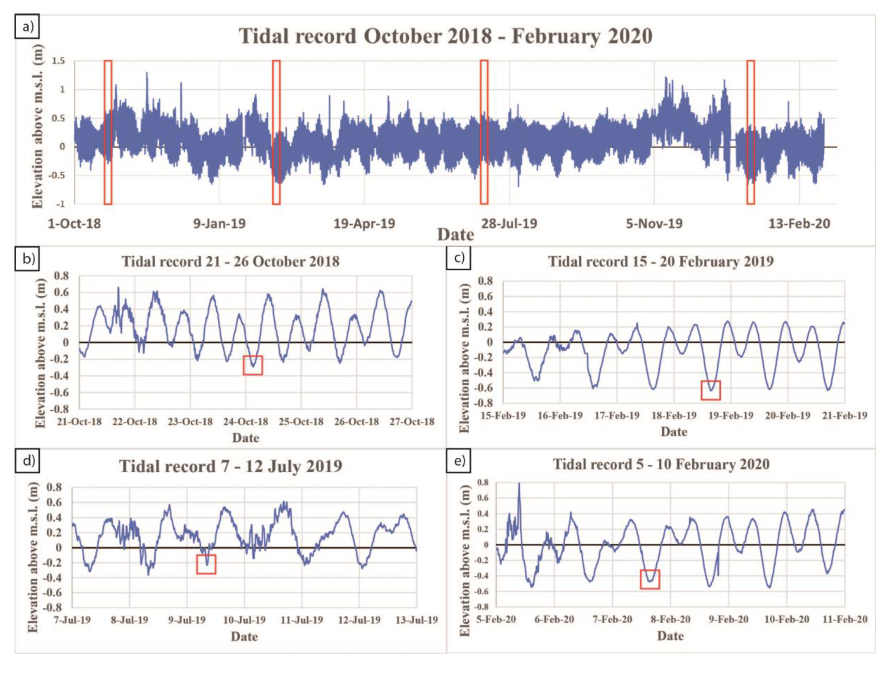
3.1. Fieldworks

The fieldwork campaigns were carried out between October 2018 and February 2020 using an aerial commercial drone (i.e., DJI Phantom Vision 3+; camera: FC300X; focal length: 3.61 mm; pixel size: 1.56 × 1.56 μm) and an RTK-GPS Trimble R8 (i.e., stop and go technique; horizontal accuracy of 8 mm and vertical accuracy of 15 mm ).
During each survey, around 80 GPS points were collected throughout the tidal flat. In this paper, they will be referred to as “validation points”, since they were used for comparison with the UAV-derived DSM products. The GCPs consisted of white and red wooden square targets, measuring 60 × 60 cm so as to be highly visible in the aerial photos; distributed around the tidal flat, their position was measured with the GPS antenna (Figure 2a). They were located within, and at the edge of, the study area—where it was possible to safely walk on the mud flat—in order to support and optimise the photogrammetry reconstruction (see Section 3.2). Additionally, a transect (Figure 2b) was surveyed along the entire study area (South-West North-East) during the last survey of February 2020. All GPS measurements (i.e., GCP and validation points) were then referenced in WGS84/UTM zone 33N (EPSG:32633). The average horizontal and vertical error associated with the measured GCP and validation points ranged between 3 and 4 cm, respectively.
In order to successfully complete a survey in coastal wetlands, many factors must combine due to water-saturated sediment surface and the reduced window of flight completion time; consequently, the surveys were carried out during spring-tides, when the moon and the sun are aligned and the lowest tides occurred and, during early morning or late afternoon, when the sun was not at its highest location in the sky; the wind speed ranged from 1.5 to 5.56 m/s during all fieldworks, thus its influence was considered negligible. Four surveys were carried out on the following dates: (i) 24 October 2018; (ii) 18 February 2019; (iii) 9 July 2019; (iv) 7 February 2020 (Figure 3). In each drone survey, thefront and the side overlap between each photo was ~70% and the flight speed was 8–10 m/s. The first survey was carried out at a height of ~80 m. During the survey of February 2019, two flights were completed, the first at ~80 m, and the second one at ~40 m. The survey of July 2019 was performed using a single flight at ~80 m. During the last survey of February 2020 two flights—at ~80 and ~60 m—were completed. The automated flights were prepared using the “Drone deploy” free application (https://www.dronedeploy.com/ accessed on: 11 June 2021), following parallel flight lines for all surveys.

3.2. Photogrammetric Tests

After each survey, the images were imported and processed using the “Agisoft Metashape” software (version 1.5.1 https://www.agisoft.com/ accessed on: 11 June 2021) which allows the generation of georeferenced DSMs and orthophotos by processing the drone images with the Structure-from-Motion (SfM) photogrammetric technique. The procedure followed previous UAV-based works, such as Fonstad et al. (2013), Casella et al. (2014), (2016), Gindraux et al. (2017) [29,73,74,75]. In general, images were aligned, GCPs were manually detected, coordinates were imported and associated with each GCP, the camera alignment was optimised, a dense cloud was generated, and the DSMs and the orthophotos were processed and exported. It is important to note that the embedded GNSS position of the images was not used since the accuracy of the UAV GNSS was not appropriate for processing, hence the camera calibration was optimized through the GCP points and, consequently, the sparse cloud was georeferenced.
In total, eight photogrammetric tests were processed based on the combination of sets of photos taken at different altitudes. The details of the tests are given in Table 1. Notably, the tests cover the whole domain, or portion of it, depending on the processed set of images or their combination.
The DSM products were cropped, removing the portions outside the area covered by the GCPs and noises derived from water. For consistency, the analysis was performed exclusively on the same area. The vegetation at the edges and the wet areas of the domain were also excluded from the models. With the term “coverage” we mean the area that is contained by the polygon defined by the GCPs located at the edge of the study area. The DSMs cover the tidal flat only and there is no vegetation inside the study area, except for rare and erratic patches of Spartina, considered insignificant due to their small size and reduced distribution. It is important to note that the B3 test has the same coverage as B1, which means that 2 ha only were processed with two sets of photos at 40 and 80 m of altitude, while the rest of the area was processed with photos at 80 m of altitude.
The photogrammetric processes and their resulting products (i.e., the DSM and the orthophotos), were referenced in WGS84/UTM zone 33N (EPSG:32633).

3.3. Validation of the DSMs

The elevation of the (GPS-based) validation points was compared with the UAV-derived DSM elevation in order to calculate the RMSE (Root Mean Square Error) (1) which, if the points are well distributed within the domain, represents a fair estimation of the accuracy of the drone-derived product:
RMSE = i = 1 n [ Z D S M Z G P S ) 2 i n
where ZDSM is the vertical elevation of the DSM and ZGPS is the vertical elevation of the GPS point.
It should be noted that, in order to test the sensitivity of the RMSE to the variations in the resolution of the DSM, the tests C, D1 and D2 were exported at three different horizontal resolutions (0.1, 0.25, and 0.5 m) and compared with the GPS data.

3.4. Comparisons between Photogrammetric Tests

The pool of processed DSMs (Section 3.2) was compared by calculating the differences between couples of DSMs. Generally, this process is applied to evaluate the morphological changes between two DSMs representative of two instants in time, and its results are referred to as DEM of Difference (DoD). In the case of the current research, the comparisons were performed between DSMs representative of the same instant in time (i.e., same day of the survey) in order to understand the sensitivity of the DSM to changes in UAV flight altitude, GCP number, and distribution. The differences were evaluated in terms of vertical and volumetric variations. The DoD as defined in this paragraph will be referred to as DEMs of Error (DoE) in the following, in order to highlight that this product refers to the variation/error due to the field and photogrammetric input. It is important to understand that the DoEs do not provide information about the evolution of the study area.
The coverage between the 40 m DSM and the others is different, consequently, two areas were examined: one of about 4.7 ha and the other one of about 1.8 ha, so the DoEs are calculated separately.

3.5. DEM of Difference: Evolution of the Area

As anticipated, a DoD represents the vertical variations of an area between two instants in time, as represented by two DSMs. For this study, four-time intervals were considered: (i) from October 2018 to February 2019, (ii) from February 2019 to July 2019, (iii) from July 2019 to February 2020 and, finally, (iv) the whole period from October 2018 to February 2020 (Figure 3). DoDs were computed and analysed to understand the evolution of the tidal flat.

3.6. Significance of the Vertical Differences

In order to evaluate the significance of the identified vertical variations, both DoEs (Section 3.4) and DoDs (Section 3.5) were computed with a tool developed by Wheaton et al. [76] called Geomorphic Change Detection (GCD). This tool estimates vertical and volume variations between DEMs, and the related uncertainties considering a threshold for change detection (TCD) below which the variations are not considered significant; thus, the most significant changes are highlighted.
This is important as calculations between DSMs cause the propagation of individual errors. By not taking into account the propagated error, DoDs (or DoEs) might provide unreliable information on the vertical and volume variations. The GCD tool provides an effective way to account for the uncertainty of the results in terms of vertical and volume changes, considering the original uncertainty/error of the input DSMs.
In this study, it is assumed that the DoDs and DoEs have a spatially constant uncertainty which is assessed by linear propagation of the uncertainty/error of the original DSMs, using the following Equation (2):
δ Z DoD / DoE = δ Z 1 2 + δ Z 2 2
where δZDoD/DoE is the propagated error, while δZ1,2 are the individual errors of the DSMs used for the calculations. The spatial uniform TCD is considered equal to the propagated error. Notably, other studies applied a statistical coefficient to the propagated error (e.g., t-value [76,77,78]) to define the TCD, thus assigning a significance level to it. In the case examined here, due to the nature of the study area, and the entity of the monitored morphological changes, the applied t-value is 1, which corresponds to a significance level of 68%, while a t-value equal to 1.96 corresponds to a significance level of 95%. Although this ensures higher confidence in the results, doubling the TCD while assessing morphological changes in such tidal environments might lead to a massive loss of data.
The GCD provides information about areal, volumetric, and vertical changes that include areas of surface lowering or raising, total and net variations, definition of the area of interest (i.e., the entire study area) and the area with detectable changes (i.e., the area with changes above the TCD) with relative uncertainties.
The differences calculated through the DoEs (Section 3.4) are expressed as the sum of all volume variations, hereby referred to as the Total Volume Variations, which was calculated considering all vertical changes (TVV), and only the significant one (TVVtcd). In the latter case, by definition, the calculations refer to the Area with Significant Variations (ASV), which corresponds to the area with detectable changes. The calculated ratio between the TVV (TVVtcd) and the entire domain (the ASV) defines the Total Average Vertical Difference (TAVD and TAVDtcd, respectively) which represents the vertical difference between the tests.
The morphological differences, evaluated through DoDs, were used to assess—in addition to the TVV—the Net Volume Variation, as the difference between deposited and eroded volumes, calculated considering all vertical changes (NVV), and only the significant ones (NVVtcd). The Vertical Rate of Change (VRC) was calculated as the ratio between the NVV and the entire domain, over the time period analysed, reproportioning it over a year. The VRC was also calculated only considering the significant changes (VRCtcd), thus using the ASV as the reference area.
Note that, because of the different coverage of the photogrammetric tests (see Section 3.4), two reference areas were considered: one of about 4.7 ha and the other one of about 1.8 ha (see Figure 2a). Thus, the GCD tool was applied accordingly (Section 4.3 and Section 4.4).

3.7. Integrated Geomorphological Interpretation

The orthophotos, volumetric analysis, and on-field observations enabled interpretation of the recent evolution of this tidal flat. All of the results were compared with the hydrometric records and the average flow discharge of Pontelagoscuro obtained from AIPO (Agenzia Interregionale per il Fiume Po), which is the nearest station to the Po Delta.
The elevation changes were compared with other microtidal flats worldwide, in particular to man-made deltas or coastal wetlands that were heavily influenced by human intervention, and the processes dominating these environments were discussed to find similarities or differences in their evolution.

4. Results

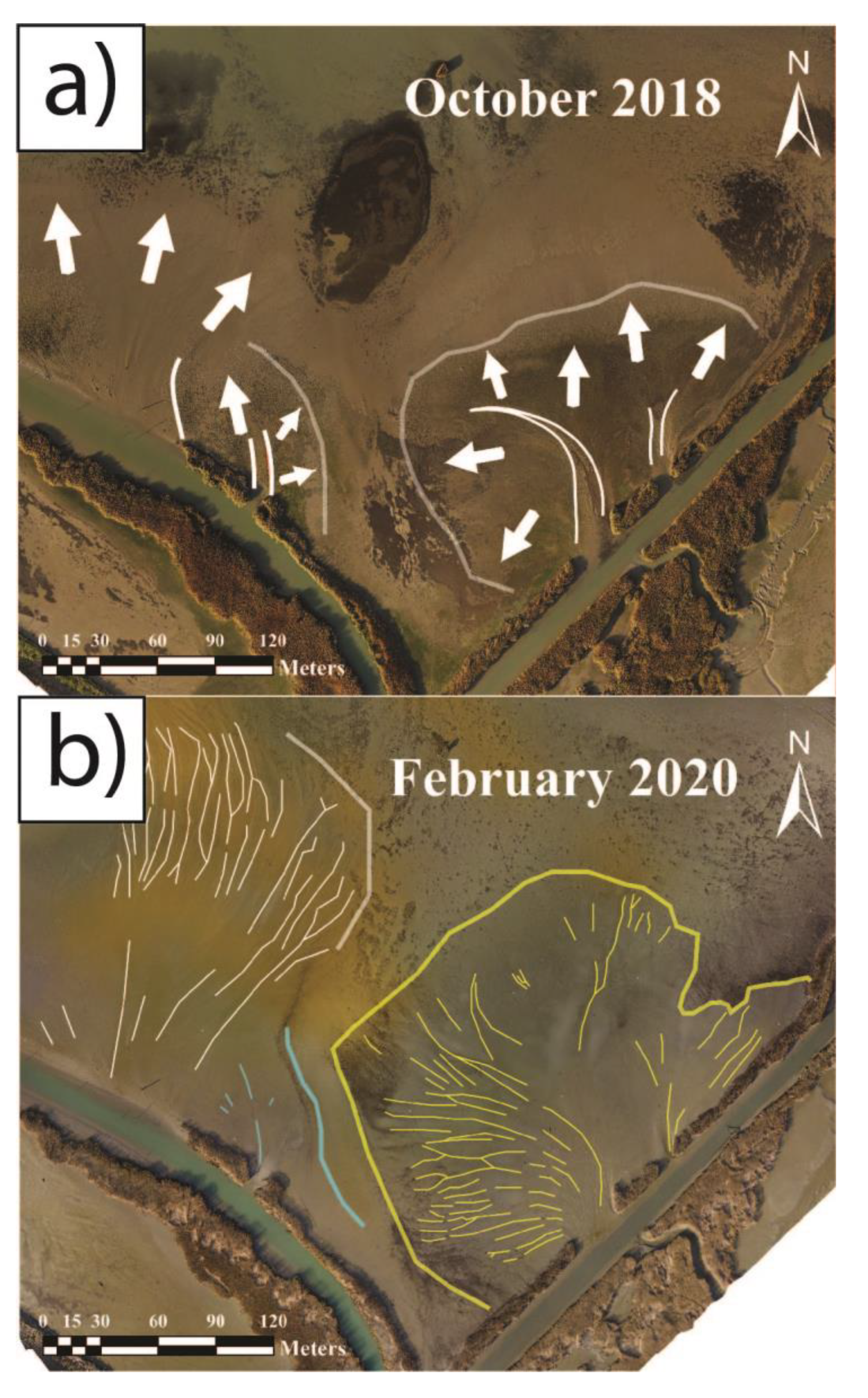
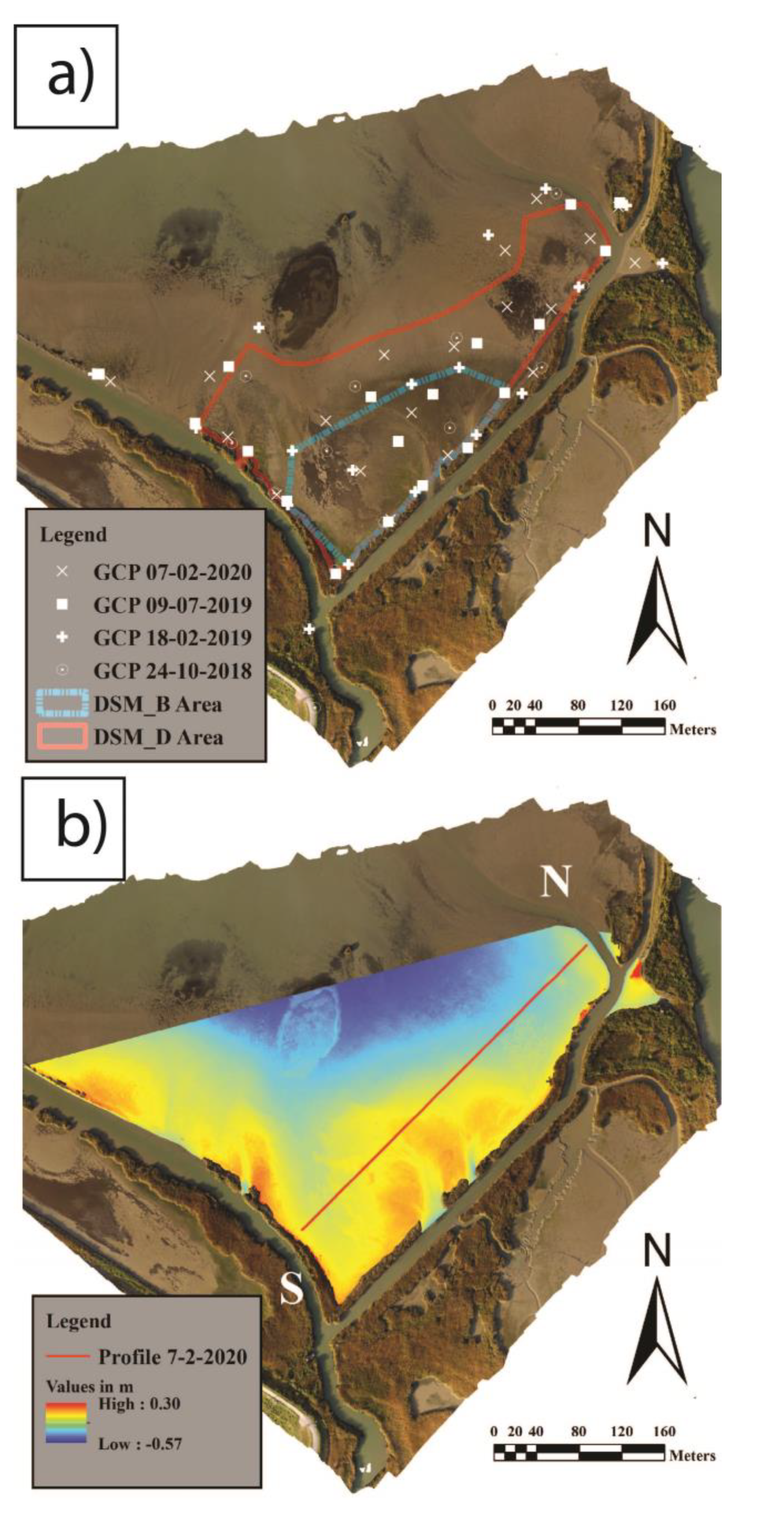
4.1. Tidal Flat Morphology

The tidal flat is protected northward by the barriers of the lagoon which prevent waves from influencing this area. The river and tidal currents are most probably the principal means of sediment transport. This observation is suggested by the presence of several crevasse splay structures that characterise the study area (Figure 4a). During floods, the sediment is brought into the tidal flat, from south to north, by four mouths located in the channels (two in the east channel and two in the west channel). The largest crevasse splay is located in the central-east zone and it is built up by both east inlets (Figure 4b in yellow); this sedimentary structure is particularly visible in the orthophoto of February 2020 after the strong flood of November-December of 2019. A second one is in the central-west zone, next to the first western mouth (Figure 4b in azure). One last large area of deposition is in the most western part, where vegetation did not completely colonise the channel levee (Figure 4b in white). Two central creeks are visible next to each inlet (except for the farther west part) where the current velocity exerts its strongest effect. The creeks are not very developed, and their length ranges from 30 to 100 m. It is notable from both orthophotos and DSMs that the creeks are developing following a NNW direction; this irregular (curved) creek shape suggests that flood influence could be higher than tidal currents alone. During high tide, the whole tidal flat is covered by water. The only vegetation able to grow in the area, excepting the levees, consists of sporadic patches of Spartina and algae. During the study period, the tidal flat did not undergo consistent alteration and the principal changes were observed in the crevasse splays.

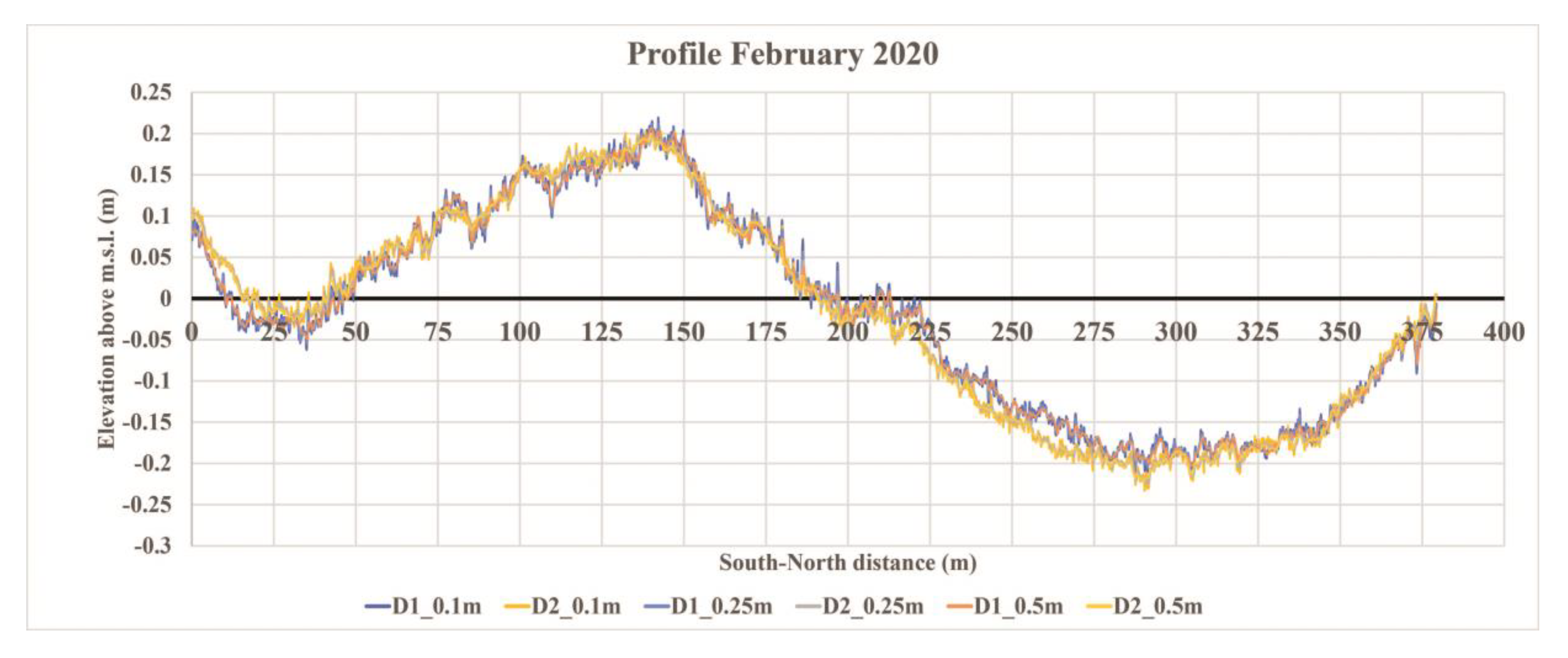
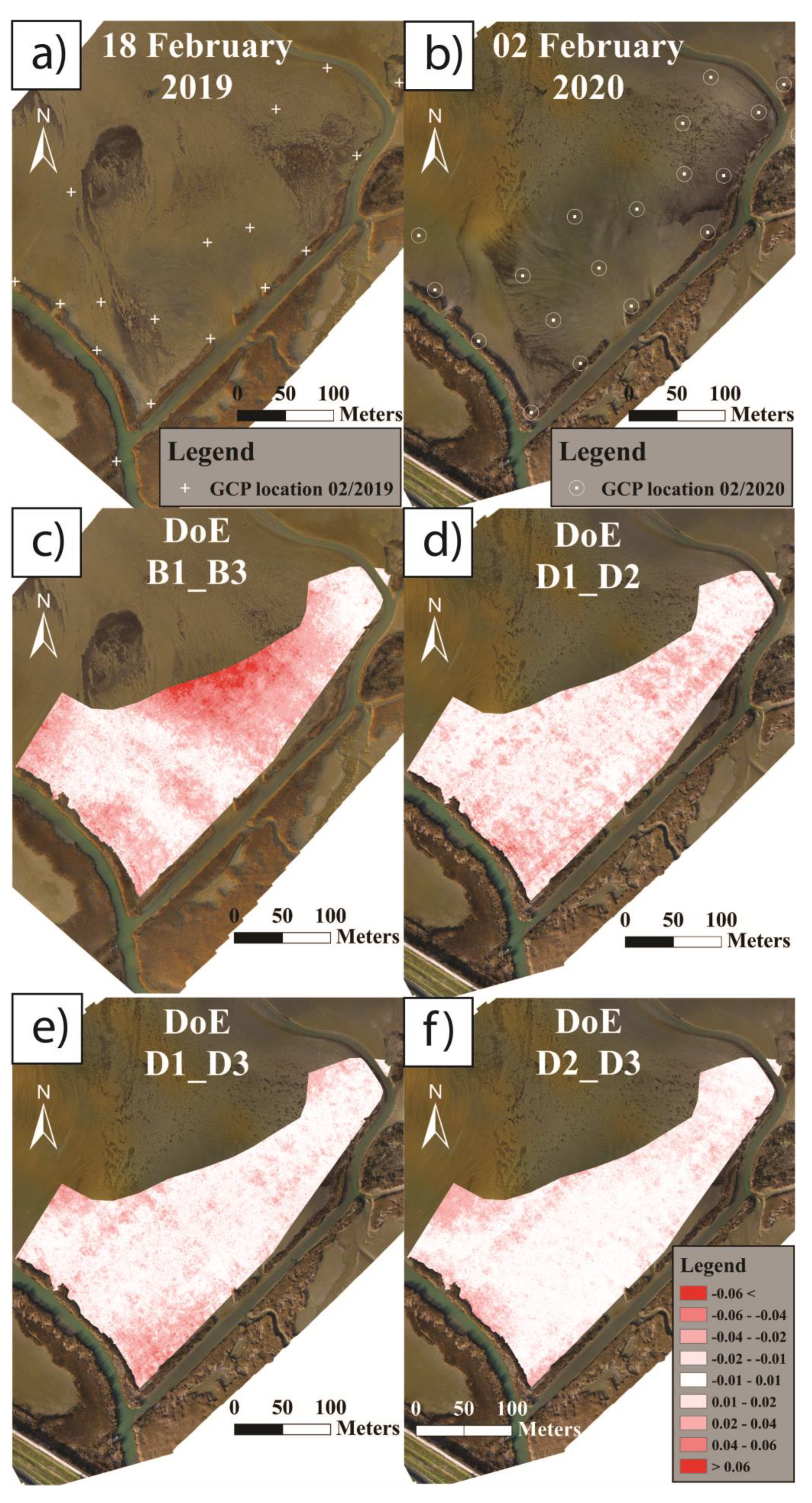
4.2. Differences due to DSM Resolution

The spatial resolution of the elevation model does not significantly affect the error calculations. The variations between the RMSEs of the same tests with 0.1, 0.25, and 0.5 m resolutions are millimetric, or sub-millimetric (Table 2). Overall, the RMSE decreases for the DSMs with a resolution of 0.5 m and it is higher for the DSM with the 0.1 m resolution; however, this variation is lower than 1 mm and might be mostly due to the smoothing process. Indeed, as expected, lower resolutions (e.g., 0.5 m) generate smoother profiles (Figure 5). While the variations arising from the different resolutions appear negligible, differences in volume estimations based on the different resolution of the input DSMs are also contained (Table 3); for example, the DoEs calculated between the D1 and D2 tests with different resolutions show volume differences in the order of 20–30 m3, which consistently decrease when only considering the significant changes (i.e., higher than the TCD), while the DoDs calculated between C and D1 or D2 show volume variations around 50 m3, which increase to ~70 m3 for the significant changes. This means that the spatial resolution of the extracted DSMs does not influence the results. The results reported in the following sections were produced using DSMs with a spatial resolution of 0.1 m.

4.3. DSM Error Assessment

Overall, the RMSEs of the analysed tests vary between 3.1 and 6 cm (Table 1). The A test based on images taken at an altitude of 80 m is characterised by one of the highest RMSE (5.7 cm), the highest coverage (8.7 ha), and the lowest density of GCPs. The B1 and the B3 tests of February 2019 have the lowest RMSE (~3 cm). It is notable that the B2 test has a higher error (6 cm) despite its showing the highest GCP density. The C test of July 2019 is based on images taken at an altitude of 80 m and shows an RMSE of 4.8 cm. This test has a higher GCP density when compared to the A test. The two flights of the last survey of February 2020 cover the same area at different altitudes (80 m and 60 m) with the same number of GCP (20 GCPs in 7.1 ha). In all D tests, the RMSE does not significantly vary more than 4 cm although it is slightly lower in the D1 test and slightly higher in the D3 test. The RMSE of the D tests is calculated using all validation points, including the transect (see Section 3.1). The accuracy does not change significantly (i.e., variations of ~1–2 mm) if the GPS points of the transect are excluded.

4.4. Differences Due to Flight Altitude

The results of the analysis of the DoEs are shown in Table 4. It is notable that the volume differences (TVV) between all tests on the 4.7 ha area range between ~475 and ~1000 m3 without applied threshold, and decreases (overall ≤ 380 m3, maximum, including uncertainty) when considering significant differences (i.e., with applied TCD) only. These values concern tests with RMSE of 3–4 cm (i.e., B1, B3, and D). The TVV increase for the DoEs concerning the B2 test (i.e., B1_B2, B2_B3): by reproportioning based on the covered area, the volume variation is ~2050 m3 (no TCD) and ~1460 m3 (with TCD, maximum, including uncertainty). Conversely, the AVDs with an applied threshold (AVDtcd) are generally higher for the D tests compared to the B ones. This is mostly due to the fact that the AVD is calculated based on the ASV, and not on the entire covered area used for regular AVD computation.
Most of the DoE values are below the threshold (Figure 6c–f), but higher values can be observed where the GCP density decreases. For example, in the northern area, where there is the largest gap in the GCP distribution, the DoE B1_B3 shows values of vertical differences between 0.1–0.15 m. The D tests are characterised by lower vertical variations, reaching a maximum of 0.05–0.1 m. Patterns can be highlighted for all the tests shown in Figure 6: there is an increase of (absolute) vertical differences moving northward, and closer to the vegetation at the borders of the south-west channel. This suggests that other factors, besides GCP distribution, may cause an increase in variations, such as, for example, the increased presence of water on the tidal flat surface moving towards the internal part of the lagoon, and the shadows due to the vegetation located at the borders of the channel.
An observation of the tests on the transect surveyed in February 2020 brings to light other details. First, the DSMs values of February 2019 were extracted based on the track of the transect surveyed one year later (Figure 7a): the vertical differences in the order of 0.1 m are visible between the B2 test and the others. The B1 and B3 tests are very similar in the first 150 m of the profile, which coincide with the B2 extension; from 150 m to 300 m the B3 test shows higher elevations with respect to B1. However, the vertical difference is about 0.05 m. The differences amongst the D tests are generally lower than 10 cm (Figure 7b); in the same figure, it is notable that most of the validation points are lower than the D tests, indicating that the DSMs generally overestimate (RMSEs ≤ 4.1 cm) the elevation of the surface when compared with GPS measurements. These lower GPS values, in particular, are probably due to a systematic error occurring during the survey when the tip of the GPS pole sinks in the mud, which is a common problem in a soft-sediment environment [47].

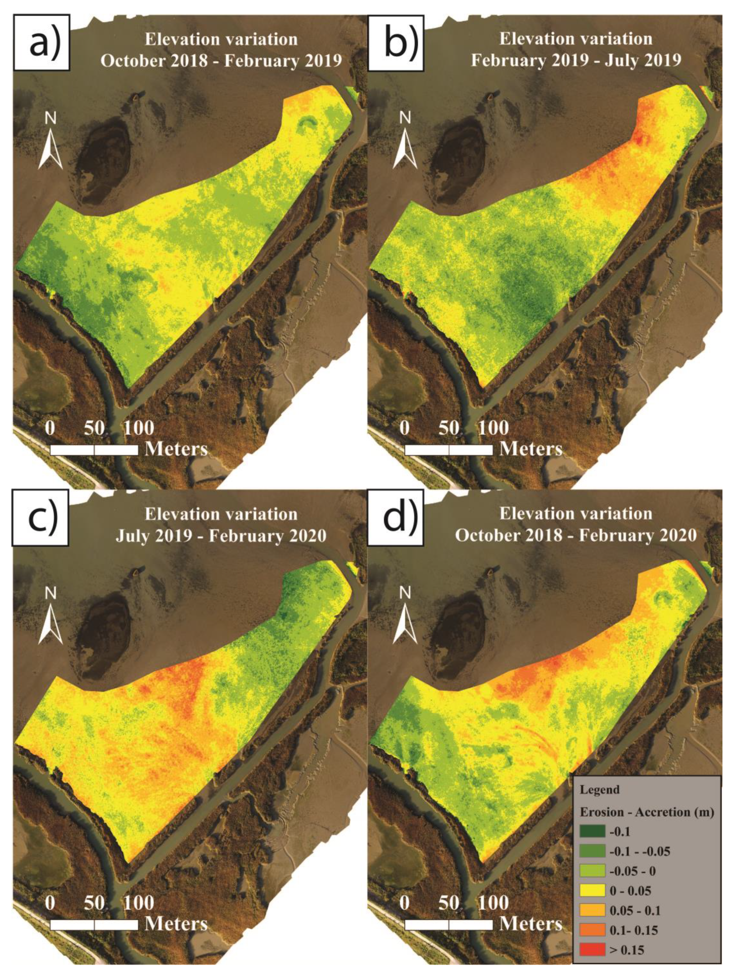
4.5. Morphological Changes

The morphological changes were analysed using DoDs (see Section 3.5) and the GCD tool (see Section 3.7), thus identifying significant vertical changes (i.e., higher than the TCD). The results are presented in the maps in Figure 8 and in Table 5. The area of interest of the analysis is ~4.72 ha. The morphological changes are analysed considering four-time intervals: i) from October 2018 to February 2019 (Figure 8a); ii) from February 2019 to July 2019 (Figure 8b); iii) from July 2019 to February 2020 (Figure 8c); and iv) the whole period from October 2018 to February 2020 (Figure 8d). The morphological changes are presented here below by focusing on net volume variations (NVV) and vertical rate of change (VRC), calculated by considering the NVV.
During the first time interval—from October 2018 to February 2019 (117 days)—the study area does not show remarkable changes. The DoDs B1-A and B3-A show—without applying TCD—two different scenarios (Table 5): one is characterised by a sediment loss of ~ 400 m3, the other shows a sediment gain of ~ 170 m3. The same DoDs analysed only considering significant changes (i.e., with applied TCD) show in both cases a sediment loss, but considering the uncertainty, the trend is not established. These values make it unclear if there is an overall erosive or accretional trend, suggesting that in these few months the tidal flat did not experience considerable changes. Nevertheless, the maps (Figure 8a) show that the sediment is moving, causing accretion in the central-northern area reaching values of 12 cm, and erosion in the south-west area, with even higher values of up to 15 cm.
The pattern is confirmed for the second period analysed, from February 2019 to July 2019 (141 days). In this case, the DoDs C-B1 and C-B3 show an erosion of ~ 95m3 and ~680 m3, considering all changes, while if only significant changes are considered, then a positive sediment budget is highlighted. However, once again, the uncertainty ranges are large and include almost null sediment budget as well as erosive trends. The erosion is quite extended throughout the central area (up to ~15 cm), while the accretion is concentrated in the northern area (up to 20 cm) (Figure 7b).
During the third time interval—from July 2019 to February 2020 (213 days)—significant changes occurred. After the period presented above, the previously described trends were reversed and the central area presented high elevation changes (up to 25 cm), while the northern area demonstrates erosion (up to 20 cm) (Figure 8c). The sediment budget is positive for all DoDs, with an average deposit of ~1300 m3 considering all changes. The evaluation of the significant changes confirms the positive pattern (average volume ~950 m3). In addition, all tests (C-D1, 2, 3) show uncertainty ranges which, although wide, do not include null or negative budgets, thus confirming the positive pattern.
Considering the whole study period—from October 2018 to February 2020 (471 days)—the tidal flat gained ~790 m3 on average when considering all changes, and ~420 m3, on average when calculating the significant changes. Although the uncertainty ranges widely diverge and do not allow incontrovertible considerations, overall the study area shows a positive trend where the principal area of accretion is located in the central-northern part characterised by vertical changes ~15 cm, while the south-west part is eroding with a similar trend that is particularly high next to the channel (>30 cm) (Figure 8d).
The net rates presented (VEC and VECtcd, Table 5) reflect the volume variations and are highly variable, since they show different trends based on the period, ranging from −3.3 to 4.6 cm/year, considering all changes. The values of VECtcd present high variability that ranges between −7.8 to 9.7 cm/year, excepting for the B1-A tests that show a higher value due to localised erosion of the mouth of the west channel (Figure 8a). The corresponding uncertainty range falls between 16.8 and 4.4 cm/year (19.8 cm/year for the B1-A test), suggesting that the evaluation is highly uncertain.

5. Discussion

5.1. Morphodynamic Interpretation

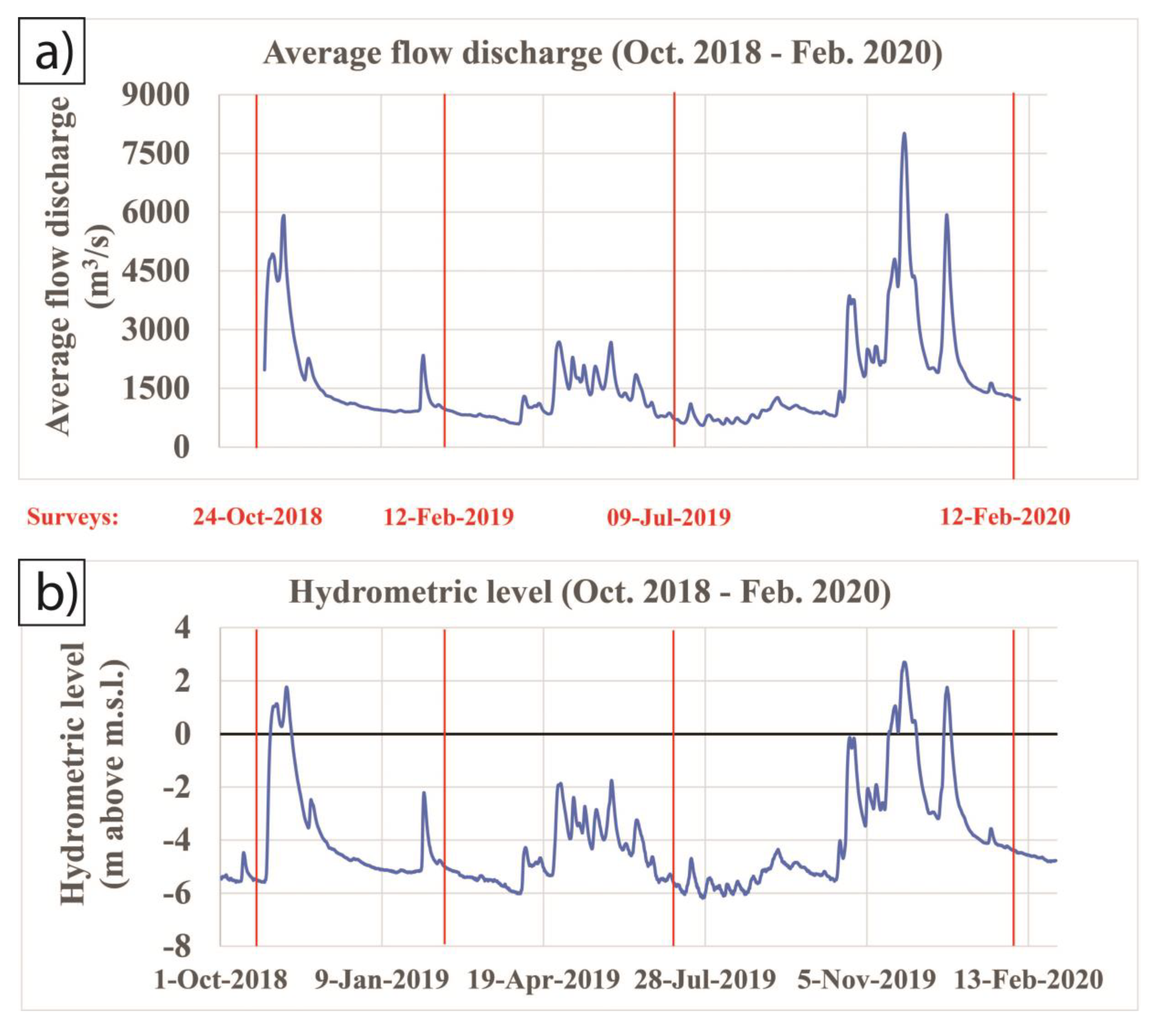
5.1.1. Tidal Flat Evolution

Tidal flats are known as dynamic environments. Nevertheless, they usually do not show remarkable morphological variations in short intervals of time (e.g., shorter than 6 months) unless a significant event occurs. Indeed, during the first 3 months of the analysed period (i.e., October 2018–February 2019), and the following 5 months (i.e., February 2019–July 2019), the Pila tidal flat did not show notable changes. The analysis was not able to clearly identify a morphodynamic trend, because of the high variability of the calculated net volumes and related uncertainty. Furthermore, the area with significant changes (i.e., exceeding the TCD) is limited (ASV max ~1.8 ha, over an area of interest of 4.7 ha). These observations do not mean that the results are uninterpretable; they suggest that it is unclear if the tidal flat underwent sediment loss or a stable condition. In both cases, during the spring–summer season, the central zone of the study area seems to have experienced sediment loss while the northern part accreted, which infers that the sediment is moving northward, inside and outside the study area.
During the remaining 8 months (July 2019–February 2020), the variations become more evident. In all cases, a positive trend is shown with high vertical rates of change (4.7 cm/year and 10.1 ± 8.8 cm/year, considering all and only significant changes, respectively), in particular in the central-northern zone.
Two principal trends seem to be followed: erosion/stability during the spring–summer season, when the tidal flat loses sediment or maintains a stable condition; and accretion during the autumn–winter season. These trends seem to coincide with the river discharge peak seasons: the most important floods caused by rainfall during winter, and weaker floods due to ice melting during the spring season [79]. In fact, it is mandatory to compare these tendencies with the hydrometric records and the average flow discharge of Pontelagoscuro obtained from AIPO (Agenzia Interregionale per il Fiume Po) (Figure 9a,b).
As shown in Table 6, the mean flow discharge and the mean hydrometric level for the whole study period were respectively about 1600 m3/s −4.1 m. In November 2018 only, there was a flood with a higher average flow discharge compared to the usual flow; the discharge peak was lower than 6000 m3/s and it lasted around 10 days. After February 2019, there were no significant floods; a few spikes are visible between April and July, probably due to small floods caused by snow melting [79,80]. On the contrary, between November and December 2019, the Po river underwent heavy flooding (> 6000 m3/s) that persisted for two months and caused a high volume of sediment transport. These events corresponded to the evolutionary trends of the tidal flat, thereby supporting the hypothesis that sediment transport is determined by river floods rather than by tides. In fact, Tesi et al. (2010) [79] showed that significant deposition in this part of the delta occurs only during large flood events; instead, only a small portion of material delivered by ordinary floods (~4000–6000 m3/s) reaches the prodelta.
Similar interpretations can be assessed for the vertical variations. The sediment loss caused an average lowering of the tidal flat of about 1.5 cm/year with significant values of 7.9 ± 15.2 cm/year during the first 8 months, followed by 4.7 cm/year with significant accretion values of 10.1 ± 8.8 cm/year during the last 8 months. Overall, the sediment budget of the tidal flat is positive for the entire analysed period, and sediment transport is particularly active in this part of the delta. The central crevasse splay is widening northward and the river seems to deposit ~800 m3/year (~420 ± 385 m3/year by considering the significant changes only) with an average vertical change rate of 1.3 cm/year (5.2 ± 4.8 cm/year by considering the significant changes only) for the whole tidal flat.
As previously explained, the DoDs were calculated reducing the domain of the DSMs to cover the same area and keep the validity of the DoDs. Unfortunately, this excludes most of the western part of the tidal flat from the analysis; hence, in order to show the vertical variations of the whole domain, the DoD between October 2018 and February 2020 was produced without filters, and it is shown in Figure 10. It is important to note that in the north-west part of the domain the GCP density is lower and the vertical variations tend to increase, as previously shown; however, these errors do not influence the reliability of a qualitative interpretation.
The small creeks are not characterised by high rates of accretion, a common behaviour expected for creeks located in natural tidal flats, which are, in themselves, in a very young stage of development. The mud platform resists flow, causing it to be concentrated into the creeks which, typically, undergo an enlarging phase [81]. Usually, the process is caused primarily by tidal currents but, in this study case, creek formation is probably owed to both river floods and ebb currents. The latter exert a greater influence on the morphology than flood tides do [82]. Moreover, this research area is characterised by river floods and ebb tide direction both moving from south to north. The sedimentological analysis of sediment samples, collected during the period covered by this study but not reported in this paper, suggests that coarser sediment is located in the internal part of the crevasse splay, while finer sediment is found moving peripherally to these areas; judging from the low amount of deposited sediment during tidal cycles, it is possible to conclude that the tide reshapes the tidal flat and moves the sediment around the lagoon, while the hydrometric and flood discharge records suggest that the river is the principal sediment source.
Notably, the central-north part of the tidal flat is the section gaining sediment, with values of accretion higher than 0.15 m; conversely, the south-west section is still subject to erosive action with high values of erosion (higher than 0.3 m) principally next to the channel levees, which, when present at all, are very low compared to the other levees. This strong erosion could be caused by fishermen boats sailing across the channels. In fact, the west channel is frequently crossed by workers needing to move through the lagoon; the waves generated influence and erode the levees, in particular, on the west side. In this section, the vegetation is absent and cannot protect the levees as it does along the other channel. This is a common problem in tidal flats or salt marshes situated close to harbours [83] or subject to intense boat traffic. Another possible reason for this strong erosion could be the formation of a new tidal creek—such as the ones seen in the inlets of the east channel—since the lack of vegetation could enable the floods and ebb tidal currents to exert a strong influence in this portion of the tidal flat.

5.1.2. Comparisons with Other Microtidal Flats

Seasonal variations are strictly connected to the driving process dominating tidal flat evolution. As an example, the Kongsmark tidal flat in Rømø Bight (Denmark) [84], a temperate microtidal environment, shows similar rates of accretion (1.5 cm/year) compared to those observed for this study case. There the controlling processes for sediment transport are the tide and the waves. However, the sediment deposition is caused by algae binding, which grows during the spring–summer period [85], while erosion occurs during the rest of the year. A different evolutionary trend is found in the Pila tidal flat since, as this study suggests, the sediment deposition is due to river floods rather than to other processes like vegetation sediment entrapment, hence accretion is higher during the autumn–winter flood periods. Despite this difference, both tidal flats show that microtidal basins are highly dynamic environments and they present high rates of accretion in short periods, reaching more than 3–4 cm/year.
A similar trend is found in the Waccassa Bay in Florida (US) [86]. This coastal wetland seems to be characterised by higher sediment deposition during summer, rather than winter, because of higher biological activity. However, sediment deposition during winter seems to be controlled by storms [87,88]. Like the previous site, these marshes seem to indicate an opposite trend compared to river-dominated marshes, since the seasonality of the processes that act as a sediment supplier is different; however, in all these environments, the sediment deposition occurs during specific periods and depends on episodic events.
The Venice Lagoon (Italy) does not show very high rates of accretion/erosion (~0.3 cm/year) [89,90,91] even though it is characterised by tidal and environmental conditions similar to the Po Delta. The lack of an important sediment supplier combined with the age of the wetland (the Venice Lagoon was formed by older consolidated salt marshes, whose higher elevation entailed decreasing sediment deposition [92]) does not allow the lagoon to undergo significant change, which is quite the contrary with respect to a tidal flat as young as the Pila one.
This important difference in sedimentation is also found in other American fluvial–deltaic landscapes such as the tidal flats of North Carolina [93], or in the Texas marshes [94], or in the Mississippi Delta in Louisiana [95,96,97] where the accretion rates are millimetric due to a sediment deficit caused by human activities.
There are some cases in which tidal and fluvial sediment supply are complementary, like in the marshes and tidal flats of the Hudson River in New York [98]. These microtidal wetlands are characterised by rates of accretion of 0.6–1.1 cm/year. The sediment is brought into the tidal flats and marshes by both river discharges and high tides. Still, the river confirms its role as the principal sediment input.
Other deltas around the Mediterranean Sea Basin present similarities to the Po Delta, such as the Rhone River Delta in Southern France [99]. This large Mediterranean delta is characterised by a microtidal range of 0.3 m and river floods strongly influence the wetland evolution. Even if the delta is a wave-dominated type, the average elevation changes are quite high (1.1 cm/year), as in the Po case. The Ebro Delta in Spain suffers from sediment budget reduction due to the construction of dams, artificial levees, dikes, and canals, just like other sites previously mentioned. This activity is impacting the resilience capability of the marsh (accretion rates between 0.1–0.6 cm/year) [100].
The results of this study are in line with Day et al. (2011) [101], who measured and compared the vertical surface changes of the previously mentioned Mediterranean deltas (i.e., Po, Rhone, and Ebro deltas) with a SET. They discovered that the highest values were located next to river channels (i.e., 1–2 cm/year for all deltas), while the non-riverine sites had lower rates (few millimetres). The accretion rates of the study area confirm these observations and, most importantly, they show that river floods can cause a very high vertical surface increase in a very short period (4.2 cm/year). They also point out how important riverine inputs contribute to salt marsh survival.
Overall, microtidal wetlands are characterised by average vertical rates of accretion that range from a few millimetres to ~1.5 cm/year. Each microtidal wetland behaviour depends on a variety of factors (i.e., tidal range, river inputs, storm occurrences, wave influence, etc.) so it is fundamental to understand the sediment transport mechanism and elevation changes in order to represent the tidal flat trend, focusing, in particular, on long-term vertical variations more than on just accretion [102,103]. It appears evident that microtidal wetlands are highly dynamic and, in most cases, their sediment transport is dominated by episodic events (i.e., storms, floods) occurring during specific seasons; the influence of these factors on the morphology seems to be higher than in meso and macrotidal environments. In fact, although tidal flats and salt marshes in high tidal regimes are influenced by seasonal variations as well, the amount of deposited sediment is more impactful (e.g., Van Proosdij (2006); Brunetta et al. (2019)) [104,105]. Microtidal wetlands need these events in order to survive. In Table 7, the previously cited studies’ vertical changes are summarised.
Despite these considerations, it is important to remember that vertical changes are strictly linked to the elevation above the mean sea level [92], which means that different portions of the wetlands present different vertical rates. The averages of the vertical variations of whole systems are useful when comparing different environments but they are inaccurate when considering the capability of marshes to keep pace with Relative Sea Level Rise (RSLR). Kirwan et al. (2016) [53] demonstrated that a static topographic representation, where the landscape does not modify with the RSLR, leads inevitably to marsh drowning; they suggest focusing the analysis on lower elevation areas because these are the most frequently flooded areas. Basically, studies should focus on distinguishing elevation changes in different vertical ranges. For example, the northern portion of the Pila tidal flat that ranges between 0.4 and −0.2 m above m.s.l. has elevation rates of 6–7 cm/year, which is a very high value compared to the whole tidal flat. Quite a different case is presented by the Lippenbroek tidal flat (NL)—an artificial tidal flat with controlled tidal amplitude (tidal range of 1.3 m), which had > 8 cm/year around 0 and 0.3 m above m.s.l. [106]. These sites are an example of how river-dominated transport can be just as important as tidal-driven sediment transport.

5.2. UAV-based Tidal Flat Monitoring

In this section, the main aspects of the approach are discussed, based on the photogrammetric tests and error assessment analysis of the UAV-based DSMs, and morphodynamical assessment. Suggestions will be given throughout this section to help researchers and practitioners in planning future field activities in tidal flats, taking into account the strengths and limitations of UAV-based surveys.

5.2.1. Field Implementation and DSM Error Assessment

The quality of a UAV-based photogrammetric product (e.g., DSM) relies on several factors, most of which are linked to environmental conditions (e.g., sunlight, presence of water on observed surfaces, etc.) and field implementation (e.g., flight planning, GCPs positioning, etc.). In this study, all of the surveys were carried out under similar environmental conditions and using the same procedure. In particular, all drone surveys were performed at the reference flight altitude of 80 m. Moreover, for some of the surveys, additional altitudes were tested (i.e., 40 and 60 m). This allowed investigation into the influence of flight altitude—and indirectly, into the number and position of the GCPs—on the accuracy of the photogrammetry-based DSMs. These parameters are all strictly correlated, and they had to be taken into account when considering the spatial and vertical accuracy of the photogrammetric products. The sensitivity analysis of the horizontal resolution (0.1, 0.25, 0.5 m) of the (exported) DSM product showed no variability in terms of error assessment (Table 2 and Table 3). The following discussion concerns DSM error assessments implemented using DSMs with 0.1 m horizontal resolution. It was found that lowering the altitude of the reference flight (i.e., 80 m), or combining sets of photos taken at different altitudes during the same day of the survey, did not necessarily reduce the error (i.e., RMSE) of the photogrammetric product (i.e., DSM), which ranged between 3 and 6 cm. For example, in both surveys of February 2019 and February 2020, the RMSEs of the B2 (40 m) and the D2 (60 m) DSMs were higher than the error of the model produced with images from an 80 m altitude (i.e., B1 and D1, respectively). The difference between B2 and B1 might have been influenced by the different coverage and GCP distribution, but for D1 and D2 the GCP density was the same. The B3 DSM (February 2019, 40 + 80 m) had the best accuracy (RMSE = 3.1 cm), but the D3 (February 2020, 60 + 80 m) presented greater error (RMSE = 4.1 cm) than the D1 (80 m). Overall, a density of ~2.8 GCP/ha enabled the error estimation (i.e., RMSE) to be limited to around 3–4 cm. Notably, higher errors were found for lower (1.9 GCP/ha) and higher (4.8 GCP/ha) density of GCPs as well. These results suggest that 80 m (but also 100 m [107], see Section 5.2.3) is a sufficient altitude to document tidal flat morphologies with UAV flights, and therefore to generate accurate photogrammetric elevation models. This reduces the flight time compared to 60 or 40 m altitude flights, and thus speeds up the field activities. However, tidal flats are commonly wide (e.g., several km), and consequently, UAV surveys can prove impracticable; therefore, it is important to find the right compromise between the required resolution and the extent of the study area.
The research herein confirmed that the number and distribution of GCPs are very important and must be considered in relation to the area being under surveyance. These findings are in line with previous works on UAV surveys [108,109]; Ablanedo et al. (2020) [109] found that neither adding higher vertical imagery nor increasing the vertical photo overlap and mixing a higher number of crossed images (in flat environments) improved the accuracy. A possible explanation of these results for this type of environment could be that the lower the flight is, the harder it will be for the SfM algorithm to identify common (i.e., tie) points between images, considering that tidal flats are quite homogeneous in terms of texture and colours. This is particularly evident in the lowest flight (B2) where, despite the high density of GCPs (i.e., 4.8 GCP/ha), the RMSE is the highest (i.e., 6 cm) (Figure 6a).

5.2.2. UAV-based Morphodynamic Assessment and Uncertainty

The differences in terms of total average vertical (TAVD) and total volume (TVV) variations highlighted for the tested DSMs (Table 4), which, on the contrary, showed similar results in terms of error assessment (RMSE; Table 1), raise questions on the reliability of the UAV-derived DSMs to perform morphodynamic assessments in such environments. For example, in terms of total volume change on the 4.7 ha area, the total average vertical difference amongst the DSMs B and D were 2 and 1 cm, respectively, while the (average) total volume difference resulted to be ~1000 m3 and ~550 m3, respectively. By only considering the significant vertical changes (i.e., higher than the TCD), the volume differences decrease, while the total average vertical difference increases. The uncertainty of these results is high.
These variations highlight that UAV-based elevation models are accompanied by a certain degree of uncertainty—due to the fieldwork implementation (i.e., flight altitude)—that must be expected and that propagates to the results of the morphodynamic assessment. This uncertainty is contained within the overall uncertainty of the elevation model (assessed through RMSE; Table 1), but the effect on the DoD results is not known a priori: it can be either irrelevant or important depending on the expected volumetric variations. The previously mentioned values of total volume variations of the D tests (TVV; Table 4), compared to the total volume variations (TVV) calculated for the morphodynamic analysis (Table 5), show that the differences in volume between D1, 2 and 3 (~550 m3) represent 25–30% of the TVV calculated for the DoDs referring to February 2020. While considering the same comparison for the B test (TVV ~1000 m3; Table 4), the percentages increase to 55–75%. This result is expected since the B2 test has a higher RMSE (6 cm). Note that these percentages do not represent the error of the calculated morphodynamic volumes, but indicate that the input DSMs have a certain degree of uncertainty (hereby expressed as TVV) that is comparable to (i.e., in the order of) the results of the morphodynamic assessment on volumes, performed by considering all changes. On the other hand, if similar comparisons are made considering the significant changes only—and thus between the TVVtcd in Table 4 and Table 5, only considering the mean value, excluding the uncertainty range—the percentages referring to the D tests decrease below 1%, while for the B tests they generally decrease, but never below 22%.
This suggests that in order to reduce the uncertainty of the final study case results—thus increasing the reliability of the assessment—UAV flights should always be performed at the same altitude (e.g., 80 m) to ensure field consistency, and consecutive surveys should be planned sufficiently distant in time so that the expected changes in elevation and volume are higher than the uncertainty generated by the field implementation (e.g., differences in flight altitude).
Indeed, as coastal wetlands slowly modify their surfaces, the vertical variations need time to occur and to be detectable via monitoring instruments depending on their characteristics. The changes depend on the entity of the accretion/erosional trend. Since each environment has different evolutionary trends, the optimal timing for a survey depends on when important morphological variations will be detectable. For example, in the Po Delta sediment is mainly transported by the river [70,71,72], so morphological variations become evident when important floods occur; hence, surveys should be carried out before providing the forecast is available ahead of time—and after the event. On the other hand, tidal currents take a much longer time to influence tidal flats, so that the time interval between one survey and the consecutive one should be longer.
Similar conclusions can be reached by considering that if the expected average vertical variations are lower than the (accepted) error of the DoD—which is assessed by propagating the (accepted) errors (i.e., RMSEs) of the analysed DSMs—it is very likely that most of the calculated vertical and volume variations are not significant, having assumed that the original DSMs are a correct representation of the reality, with acceptable errors. Thus, in general, the period between two consecutive surveys should be calibrated based on the expected variations and the expected error of the DSMs. As a simplified example, the case documented here assumes that the representative expected rate of variation can be assessed by calculating the TAVD (Section 3.6) with the TVV in Table 5 for the entire analysed period (October 2018–February 2020), reproportioning it over one year, and dividing it by 2 (thus assuming null NVV, i.e., equal eroded and deposited volumes), producing a result of ~1.4 cm/year; since the average error (i.e., RMSE) of the UAV-based DSMs was ~5 cm and, the propagated DoD error between two DEMs is ~7 cm, the shortest period between consecutive UAV surveys, can be roughly estimated as 7 [cm]/1.4 [cm/year] = 5 [years]. This is, of course, unfeasible. However, if the calculation takes into account the uncertainty, meaning that non-significant changes are excluded from the analysis (e.g., using the methods applied for this study), this period decreases. For the previous example, considering the TVVtcd—which is representative of the areas with significant changes only (ASV)—the representative expected variation is 3.8 (±2.7) cm/year, thus, the previous assessment leads to 1.8 (±2.6) years needed between one UAV survey and the consecutive one. Notably, this range is comparable with the entire period analysed in this study (~1.3 years). If the representative expected variations are calculated for all the other periods considered in this study, and the mean values, including uncertainty, are considered, the representative expected variation results 11.4 (±7.1) and it leads to 0.6 (±1.0) years. Indeed, the seasonal variations of the Pila tidal flat were documented through sub-annual surveys.
This experimentation demonstrates that the UAV is a suitable tool to monitor tidal flat morphodynamics when sub-annual variations are expected to be higher than the error propagation. However, this is only valid if the accuracy is assessed and monitored throughout the entire process. Notably, the morphodynamic interpretation (Section 5.1) of the case study documented here and the considerations collected in this section were made possible because the elevation model uncertainty was thoroughly analysed and tracked throughout the entire process. This research feature, in particular, made it possible to evaluate the effect of some aspects of the field implementation on the DSM accuracy and to detect significant changes to perform accurate and reliable morphodynamic interpretations. It is therefore suggested to take uncertainty into account while processing UAV surveys for morphodynamic monitoring on tidal flats, and other environments.

5.2.3. Comparisons with Other Studies with UAV in Wetlands

Fieldwork in tidal flats and salt marshes is usually very challenging and needs to be well organised. Beyond its mere feasibility, a survey should be organised considering two principal aspects: the extension of the study area, and the significance of the expected vertical changes. It is very important to consider the rates of changes because they determine the resolution needed for the study which would, otherwise, produce unreliable data. However, a longer time interval between surveys can correct the imbalance among these rates of change. For example, the Venice Lagoon (Italy) has a very low rate of accretion ranging between millimetres and a few centimetres per year [90,91] which means that even UAV surveys would have difficulty evaluating volume and vertical changes; this is the reason why different on-field methodologies, like sedimentation plates, are used in the Venetian lagoon. The opposite situation can be found in the Perkpolder tidal basin (Netherlands) where the sedimentation rates are very high (> 6 cm/year) and constant; wide vertical changes allow Lidar methodology to be quite accurate with a time interval of one year [105]. As explained in the previous section, it is necessary to find a compromise between the extent of the study area and the resolution of the survey. An overview of datasets for similar intertidal environments from the literature is shown in Table 8.
In producing a reliable survey, flying at a low altitude (e.g., 20–30 m) seemed less important [109] compared to GCP density, spatial distribution, and flight plan which, by contrast, appeared to be driving factors. Other salt marsh research with UAVs has been carried out at very low heights with a GCP distribution and density comparable to this study; we recall here Brunier et al. (2020) [110] and Kalacska et al. (2017) [46]. They flew, respectively, at 18 and 30 m of altitude, with a GCP density of 4.6 and 2.8 GCP per hectare. Their estimation of RMSE is very low (2.7 and 3.4 cm) but it is no more precise than the error calculations of this study at higher altitudes (i.e., 60–80 m). Furthermore, in this study as well, the lowest flight at 40 m with 4.8 GCP/ha did not achieve higher accuracy. The same RMSE can also be achieved at higher altitudes, as shown in the Jaud et al. (2016) [107] case. They conducted a very similar survey in an area of ~10 ha flying at 100 m and with a GCP density of 1.5 GCP/ha and were able to reach an error ranging between 3.9 and 2.7 cm. In other studies where the UAVs flew at higher altitudes, between 80 to 180 m, and the GCP density was very low (below 0.2 GCP/ha), the error increased to 10–20 cm till 5 m [111,112,113]. The relation between GCP density and RMSE from the previously cited researches is shown in Figure 11. These comparisons suggest that centimetric errors (e.g., 2.7–6 cm) can be achieved with UAV flight altitudes from 20 to 100 m. Even though it could be possible to increase accuracy at heights lower than 20 m, either the fieldwork would prove extremely long or the area would have to be highly restrained; nevertheless, proper foresight can simplify the survey and ensure it achieves a very good quality. The distribution of the GCPs for Brunier et al. (2020) [110] and Jaud et al. (2016) [107] was homogeneous and the distance between each GCP was mostly coherent, which probably resulted in achieving a low RMSE (i.e., 3–4 cm). In studies with greatly extended areas, the GCP distribution was neither dense [112] nor homogeneous [111,113], causing higher RMSE (i.e., >10 cm). The best GCP distribution seems to be around ~2.5 and 3 GCP/ha, which is 2–3 GCP every 100 m homogeneously and equally spaced around the tidal flat.

5.2.4. Recommendations for UAV surveys in wetlands

The discussion of the results and the limitations of the general approach brought us to make considerations about UAV surveys in wetlands and thus recommendations are proposed to optimize the data acquisition. The following points are suggested:
  • The fieldwork should be planned in the function of the expected rate of changes and the time between each survey based on the knowledge of the area;
  • A comparison with ground-truthing (e.g., vs. GPS) is always recommended;
  • 2–3 GCPs should be located every 100 m homogeneously and equally distributed in order to reach centimetric RMSE;
  • The flight can be carried out at 80–100 m altitude to save time but the altitude must be kept constant for the whole monitored period;
  • The fieldwork should be carried out during the early morning or late afternoon time slots, and with cloudy weather when a spring low tide occurs.
These guidelines can help researchers and practitioners in planning field activities in such environments, taking into account the strengths and limitations of UAV-based surveys. Notably, such guidelines must be considered non-definitive since additional research on UAV applications should be envisaged, particularly with regard to developing thorough uncertainty assessments.

6. Conclusions

Over the last 50 years, the Po River Delta has been subjected to alternating phases of erosion and progradation. During the last decade, the delta has been accreting, and new tidal flats are forming. This study concerns an 8 ha young tidal flat that stretches northward from the southern part of the Barbamarco Lagoon to the Po della Pila branch in the Po Delta (Figure 1). From October 2018 to February 2020, four UAV surveys were carried out at different altitudes and with different GCP numbers and distribution. Eight photogrammetric tests were performed in order to evaluate the uncertainty and accuracy of the elevation models and related morphodynamic assessments. The volumetric and elevation changes were evaluated considering the whole study area and the area with significant changes, which are defined as the vertical changes higher, in the module, than an established threshold. The threshold was evaluated on the basis of the propagation of the error of the input DSMs.
The principal conclusions of this research on the morphodynamics of the analysed portion of the Pila tidal flat are the following ones:
  • During the last phase part of the winter season and the spring–summer season of 2018–2019, the study area experienced erosion while in the autumn–winter season of 2019–2020 an accretion trend was predominant. Timewise, the increase and the widening of the tidal flat coincide with the heavy flood events occurring in the Po River during November–December 2019;
  • Overall, the sediment budget is positive, and the tidal flat is gaining ~800 m3/year with an average accretion rate of 1.3 cm/year (by considering the significant variations those values become 420 ± 385 m3/year and 5.2 ± 4.8 cm/year, respectively);
  • The accretion trends of the tidal flat of Pila are similar to other microtidal deltas worldwide; most of them are characterised by seasonal variations that depend on episodic events (i.e., floods, storms) and do not present constant trends like tide-dominated deltas.
The above points were supported by a thorough assessment of the accuracy of the UAV-based DSMs and of the calculated volume changes. In regard to this, the RMSE (vs. GPS measurements) of the DSMs ranged between 3 and 6 cm. The accuracy of the DSMs was not dependant on the altitude of the UAV flight, but rather on the number and distribution of the GCPs.

Author Contributions

R.B.: Conceptualisation, Data curation, Formal analysis, Investigation, Methodology, Writing—review and editing. E.D.: Methodology, Formal analysis, investigation, Writing—review and editing. P.C.: Funding acquisition, Supervision, Writing—review and editing. All authors have read and agreed to the published version of the manuscript.

Funding

This research was supported by the project ‘‘Dipartimenti di Eccellenza 2018–2022”of the Italian Ministry of Education (MIUR), awarded to the Department of Physics and Earth Sciences of University of Ferrara.

Data Availability Statement

The data presented in this study are available on request from the corresponding author.

Acknowledgments

The authors thank Guido Selvi and Vittorio Negri of the Genio civile di Rovigo for the logistical support essential to the purpose of this study. Particular thanks go to Edoardo Grottoli and Stefano Fabbri for their suggestions and help in the field. Important help during the fieldwork was provided by Lorenzo Franzoni, Asrat Asresu, Enrico Ferrari, Francesco Miricola.

Conflicts of Interest

The authors declare that no financial interests or personal relationships influenced the research reported in this paper.

References

  1. Dyer, K.; Christie, M.; Wright, E. The classification of intertidal mudflats. Cont. Shelf Res. 2000, 20, 1039–1060. [Google Scholar] [CrossRef]
  2. Pratolongo, P.; Leonardi, N.; Kirby, J.R.; Plater, A. Temperate Coastal Wetlands. In Coastal Wetlands; Elsevier: Amsterdam, The Netherlands, 2019; pp. 105–152. [Google Scholar]
  3. French, J.R. Saltmarshes: Morphodynamics, Conservation and Engineering Significance; Allen, J.R.L., Pye, K., Eds.; Cambridge University Press: Cambridge, UK, 1992. [Google Scholar]
  4. Adam, P. Plant Life History Studies; Cambridge University Press: Cambridge, UK, 1990; pp. 309–334. [Google Scholar]
  5. Odum, W.E.; McIvor, C.C.; Smith, T.J. The Ecology of the Mangroves of South Florida: A Community Profile. U.S. Fish and Wildlife Service; Office of Biological Services: Washington, DC, USA, 1982; p. 156. [Google Scholar]
  6. Christiansen, T.; Wiberg, P.; Milligan, T. Flow and Sediment Transport on a Tidal Salt Marsh Surface. Estuar. Coast. Shelf Sci. 2000, 50, 315–331. [Google Scholar] [CrossRef] [Green Version]
  7. Leonard, L.A.; Wren, P.A.; Beavers, R.L. Flow Dynamics and Sedimentation in Spartina alterniflora and Phragmites australis marshes of the Chesapeake Bay. Wetlands 2002, 22, 415–424. [Google Scholar] [CrossRef]
  8. Temmerman, S.; Govers, G.; Wartel, S.; Meire, P. Modelling estuarine variations in tidal marsh sedimentation: Response to changing sea level and suspended sediment concentrations. Mar. Geol. 2004, 212, 1–19. [Google Scholar] [CrossRef]
  9. Boesch, D.F.; Turner, R.E. Dependence of Fishery Species on Salt Marshes: The Role of Food and Refuge. Estuaries 1984, 7, 460–468. [Google Scholar] [CrossRef]
  10. MacKenzie, R.; Dionne, M. Habitat heterogeneity: Importance of salt marsh pools and high marsh surfaces to fish production in two Gulf of Maine salt marshes. Mar. Ecol. Prog. Ser. 2008, 368, 217–230. [Google Scholar] [CrossRef]
  11. Barbier, E.B.; Hacker, S.D.; Kennedy, C.; Koch, E.W.; Stier, A.C.; Silliman, B.R. The value of estuarine and coastal ecosystem services. Ecol. Monogr. 2011, 81, 169–193. [Google Scholar] [CrossRef]
  12. Mayor, J.R.; Hicks, C.E. Potential Impacts of Elevated CO2 on Plant Interactions, Sustained Growth, and Carbon Cycling in Salt Marsh Ecosystems, Human Impacts on Salt Marshes A Global Perspective; Silliman, B.R., Grosholz, E.D., Bertness, M.D., Eds.; University of California: Berkeley, CA, USA, 2009; pp. 207–228. [Google Scholar]
  13. Weis, P. Salt Marsh Accretion. In Encyclopedia of Solid Earth Geophysics; Springer: Berlin/Heidelberg, Germany, 2016; pp. 513–515. [Google Scholar]
  14. Bouma, T.J.; van Belzen, J.; Balke, T.; Zhu, Z.; Airoldi, L.; Blight, A.J.; Davies, A.J.; Galvan, C.; Hawkins, S.J.; Hoggart, S.P.; et al. Identifying knowledge gaps hampering application of intertidal habitats in coastal protection: Opportunities & steps to take. Coast. Eng. 2014, 87, 147–157. [Google Scholar] [CrossRef]
  15. Möller, I.; Kudella, M.; Rupprecht, F.; Spencer, T.; Paul, M.; Van Wesenbeeck, B.K.; Wolters, G.; Jensen, K.; Bouma, T.J.; Miranda-Lange, M.; et al. Wave attenuation over coastal salt marshes under storm surge conditions. Nat. Geosci. 2014, 7, 727–731. [Google Scholar] [CrossRef] [Green Version]
  16. Van Loon-Steensma, J.M. Salt Marshes for Flood Protection; Wageningen University: Wageingen, The Netherlands, 2014; p. 203. [Google Scholar]
  17. Smolders, S.; Plancke, Y.; Ides, S.; Meire, P.; Temmerman, S. Role of intertidal wetlands for tidal and storm tide attenuation along a confined estuary: A model study. Nat. Hazards Earth Syst. Sci. 2015, 15, 1659–1675. [Google Scholar] [CrossRef] [Green Version]
  18. Stark, J.; Van Oyen, T.; Meire, P.; Temmerman, S. Observations of tidal and storm surge attenuation in a large tidal marsh. Limnol. Oceanogr. 2015, 60, 1371–1381. [Google Scholar] [CrossRef]
  19. Vuik, V.; Jonkman, S.N.; Van Vuren, S. Nature-based flood protection: Using vegetated foreshores for reducing coastal risk. E3S Web Conf. 2016, 7, 13014. [Google Scholar] [CrossRef] [Green Version]
  20. Leonardi, N.; Carnacina, I.; Donatelli, C.; Ganju, N.; Plater, A.J.; Schuerch, M.; Temmerman, S. Dynamic interactions between coastal storms and salt marshes: A review. Geomorphology. 2018, 301, 92–107. [Google Scholar] [CrossRef] [Green Version]
  21. Millennium Ecosystem Assessment. Ecosystems and Human Well-Being: Synthesis; Island Press: Washington, DC, USA, 2005. [Google Scholar]
  22. Eisenbeiss, H. UAV Photogrammetry 2009. Ph.D. Thesis, ETH Zürich, Zürich, Switzerland, 2009. [Google Scholar]
  23. Westoby, M.J.; Brasington, J.; Glasser, N.F.; Hambrey, M.J.; Reynolds, J.M. Structure-from-Motion photogrammetry: A low-cost, effective tool for geoscience applications. Geomorphology 2012, 179, 300–314. [Google Scholar] [CrossRef] [Green Version]
  24. Moloney, J.G.; Hilton, M.J.; Sirguey, P.; Simons-Smith, T. Coastal Dune Surveying Using a Low-Cost Remotely Piloted Aerial System (RPAS). J. Coast. Res. 2018, 345, 1244–1255. [Google Scholar] [CrossRef]
  25. Mancini, F.; Dubbini, M.; Gattelli, M.; Stecchi, F.; Fabbri, S.; Gabbianelli, G. Using Unmanned Aerial Vehicles (UAV) for High-Resolution Reconstruction of Topography: The Structure from Motion Approach on Coastal Environments. Remote Sens. 2013, 5, 6880–6898. [Google Scholar] [CrossRef] [Green Version]
  26. Joyce, K.E.; Duce, S.; Leahy, S.M.; Leon, J.; Maier, S.W. Principles and practice of acquiring drone-based image data in marine environments. Mar. Freshw. Res. 2019, 70, 952–963. [Google Scholar] [CrossRef]
  27. Javernick, L.; Brasington, J.; Caruso, B. Modeling the topography of shallow braided rivers using Structure-from-Motion photogrammetry. Geomorphology 2014, 213, 166–182. [Google Scholar] [CrossRef]
  28. Ryan, J.C.; Hubbard, A.L.; Box, J.; Todd, J.; Christoffersen, P.; Carr, J.R.; Holt, T.O.; Snooke, N. UAV photogrammetry and structure from motion to assess calving dynamics at Store Glacier, a large outlet draining the Greenland ice sheet. Cryosphere 2015, 9, 1–11. [Google Scholar] [CrossRef] [Green Version]
  29. Casella, E.; Rovere, A.; Pedroncini, A.; Stark, C.P.; Casella, M.; Ferrari, M.; Firpo, M. Drones as tools for monitoring beach topography changes in the Ligurian Sea (NW Mediterranean). Geo Lett. 2016, 36, 151–163. [Google Scholar] [CrossRef]
  30. Dąbski, M.; Zmarz, A.; Pabjanek, P.; Korczak-Abshire, M.; Karsznia, I.; Chwedorzewska, K.J. UAV-based detection and spatial analyses of periglacial landforms on Demay Point (King George Island, South Shetland Islands, Antarctica). Geomorphology 2017, 290, 29–38. [Google Scholar] [CrossRef]
  31. Duo, E.; Trembanis, A.C.; Dohner, S.; Grottoli, E.; Ciavola, P. Local-scale post-event assessments with GPS and UAV-based quick-response surveys: A pilot case from the Emilia–Romagna (Italy) coast. Nat. Hazards Earth Syst. Sci. 2018, 18, 2969–2989. [Google Scholar] [CrossRef] [Green Version]
  32. Klemas, V.V. Remote Sensing of Coastal Ecosystems and Environments. In Coastal Wetlands: Alteration and Remediation; Springer: Berlin/Heidelberg, Germany, 2014; Volume 9, pp. 3–30. [Google Scholar]
  33. Adam, E.; Mutanga, O.; Rugege, D. Multispectral and hyperspectral remote sensing for identification and mapping of wetland vegetation: A review. Wetl. Ecol. Manag. 2010, 18, 281–296. [Google Scholar] [CrossRef]
  34. Ghosh, S.; Mishra, D.R. Analyzing the Long-Term Phenological Trends of Salt Marsh Ecosystem across Coastal Louisiana. Remote Sens. 2017, 9, 1340. [Google Scholar] [CrossRef] [Green Version]
  35. Duffy, J.P.; Pratt, L.; Anderson, K.; Land, P.E.; Shutler, J.D. Spatial assessment of intertidal seagrass meadows using optical imaging systems and a lightweight drone. Estuar. Coast. Shelf Sci. 2018, 200, 169–180. [Google Scholar] [CrossRef]
  36. Doughty, C.L.; Cavanaugh, K.C. Mapping Coastal Wetland Biomass from High Resolution Unmanned Aerial Vehicle (UAV) Imagery. Remote Sens. 2019, 11, 540. [Google Scholar] [CrossRef] [Green Version]
  37. Ozesmi, S.L.; Bauer, M.E. Satellite remote sensing of wetlands. Wetl. Ecol. Manag. 2002, 10, 381–402. [Google Scholar] [CrossRef]
  38. Campbell, A.; Wang, Y. High Spatial Resolution Remote Sensing for Salt Marsh Mapping and Change Analysis at Fire Island National Seashore. Remote Sens. 2019, 11, 1107. [Google Scholar] [CrossRef] [Green Version]
  39. Morris, J.T.; Porter, D.; Neet, M.; Noble, P.A.; Schmidt, L.; Lapine, L.A.; Jensen, J.R. Integrating LIDAR elevation data, multi-spectral imagery and neural network modelling for marsh characterization. Int. J. Remote Sens. 2005, 26, 5221–5234. [Google Scholar] [CrossRef]
  40. Rosso, P.; Ustin, S.; Hastings, A. Use of lidar to study changes associated with Spartina invasion in San Francisco Bay marshes. Remote Sens. Environ. 2006, 100, 295–306. [Google Scholar] [CrossRef]
  41. Wang, C.; Menenti, M.; Stoll, M.-P.; Feola, A.; Belluco, E.; Marani, M. Separation of Ground and Low Vegetation Signatures in LiDAR Measurements of Salt-Marsh Environments. IEEE Trans. Geosci. Remote Sens. 2009, 47, 2014–2023. [Google Scholar] [CrossRef]
  42. Millard, K.; Redden, A.M.; Webster, T.; Stewart, H. Use of GIS and high resolution LiDAR in salt marsh restoration site suitability assessments in the upper Bay of Fundy, Canada. Wetl. Ecol. Manag. 2013, 21, 243–262. [Google Scholar] [CrossRef]
  43. Fernandez-Nunez, M.; Burningham, H.; Zujar, J.O. Improving accuracy of LiDAR-derived digital terrain models for saltmarsh management. J. Coast. Conserv. 2017, 21, 209–222. [Google Scholar] [CrossRef]
  44. Nolte, S.; Koppenaal, E.C.; Esselink, P.; Dijkema, K.S.; Schuerch, M.; De Groot, A.V.; Bakker, J.P.; Temmerman, S. Measuring sedimentation in tidal marshes: A review on methods and their applicability in biogeomorphological studies. J. Coast. Conserv. 2013, 17, 301–325. [Google Scholar] [CrossRef]
  45. Green, D.; Mauquoy, D.; Hagon, J.; Angus, S.; Hansom, J.; Rennie, A.; Gourlay, C. Monitoring, Mapping and Modelling Saltmarsh: The UAV Way; Geomares Publishing UK Ltd: St. Albans, UK, 2017; pp. 22–28. [Google Scholar]
  46. Kalacska, M.; Chmura, G.; Lucanus, O.; Bérubé, D.; Arroyo-Mora, J. Structure from motion will revolutionize analyses of tidal wetland landscapes. Remote Sens. Environ. 2017, 199, 14–24. [Google Scholar] [CrossRef]
  47. Casella, E.; Drechsel, J.; Winter, C.; Benninghoff, M.; Rovere, A. Accuracy of sand beach topography surveying by drones and photogrammetry. Geo-Mar. Lett. 2020, 40, 255–268. [Google Scholar] [CrossRef] [Green Version]
  48. James, M.; Robson, S.; D’Oleire-Oltmanns, S.; Niethammer, U. Optimising UAV topographic surveys processed with structure-from-motion: Ground control quality, quantity and bundle adjustment. Geomorphology 2017, 280, 51–66. [Google Scholar] [CrossRef] [Green Version]
  49. Mount, R. Acquisition of Through-water Aerial Survey Images. Photogramm. Eng. Remote Sens. 2005, 71, 1407–1415. [Google Scholar] [CrossRef]
  50. Nardin, W.; Edmonds, D.A. Optimum vegetation height and density for inorganic sedimentation in deltaic marshes. Nat. Geosci. 2014, 7, 722–726. [Google Scholar] [CrossRef]
  51. Crosby, S.C.; Sax, D.F.; Palmer, M.E.; Booth, H.S.; Deegan, L.A.; Bertness, M.D.; Leslie, H.M. Salt marsh persistence is threatened by predicted sea-level rise. Estuar. Coast. Shelf Sci. 2016, 181, 93–99. [Google Scholar] [CrossRef] [Green Version]
  52. Spencer, T.; Schuerch, M.; Nicholls, R.J.; Hinkel, J.; Lincke, D.; Vafeidis, A.; Reef, R.; McFadden, L.; Brown, S. Global coastal wetland change under sea-level rise and related stresses: The DIVA Wetland Change Model. Glob. Planet. Chang. 2016, 139, 15–30. [Google Scholar] [CrossRef] [Green Version]
  53. Kirwan, M.L.; Temmerman, S.; Skeehan, M.L.K.E.E.; Guntenspergen, G.R.; Fagherazzi, S. Overestimation of marsh vulnerability to sea level rise. Nat. Clim. Chang. 2016, 6, 253–260. [Google Scholar] [CrossRef]
  54. Cencini, C. Physical Processes and Human Activities in the Evolution of the Po Delta, Italy. J. Coast. Res. 1998, 14, 774–793. [Google Scholar] [CrossRef]
  55. Simeoni, U.; Corbau, C. A review of the Delta Po evolution (Italy) related to climatic changes and human impacts. Geomorphology 2009, 107, 64–71. [Google Scholar] [CrossRef]
  56. Bondesan, M. L’area deltizia padana: Caratteri geografici e geomorfologici. In Il Parco del Delta del po. Studi e Immagini. L’ambiente Come Risorsa; Spazio Libri: Ferrara, Italy, 1990; Volume 16, pp. 10–48. [Google Scholar]
  57. Ludwig, W.; Dumont, E.; Meybeck, M.; Heussner, S. River discharges of water and nutrients to the Mediterranean and Black Sea: Major drivers for ecosystem changes during past and future decades? Prog. Oceanogr. 2009, 80, 199–217. [Google Scholar] [CrossRef]
  58. Dal Cin, R.I. Litorali Del Delta Del Po e Alle Fois Dell’ Adige e Del Brenta: Caratteri Tessiturali e Dispersione Dei Sedimenti, Cause Dell’arretramento e Preisioni Sull’ Evoluzione Futura. Boll. Soc. Geol. Ital. 1983, 102, 9–56. [Google Scholar]
  59. Simeoni, U.; Fontolan, G.; Dal Cin, R.; Calderoni, G.; Zamariolo, A. Dinamica sedimentaria dell’area di Goro (Delta del Po). Studi Costieri 2000, 2, 139–151. [Google Scholar]
  60. Simeoni, U.; Gabbianelli, G.; Tessari, U.; Calderoni, G.; Grande, C. Un Bacile di nome Delta. La Sacca di Goro. Studi Costieri 2000, 2, 31–44. [Google Scholar]
  61. Stefani, M.; Vincenzi, S. The interplay of eustasy, climate and human activity in the late Quaternary depositional evolution and sedimentary architecture of the Po Delta system. Mar. Geol. 2005, 222-223, 19–48. [Google Scholar] [CrossRef]
  62. Maselli, V.; Trincardi, F. Man made deltas. Sci. Rep. 2013, 3, 1926. [Google Scholar] [CrossRef] [Green Version]
  63. Visentini, M. Ricerche Idrografiche nel Delta del Po. Ufficio Idrografico del Po-Parma; Istituto Poligrafico Dello Stato: Roma, Italy, 1940; Volume 14, p. 175. [Google Scholar]
  64. Billi, P.; Fazzini, M. Global change and river flow in Italy. Glob. Planet. Chang. 2017, 155, 234–246. [Google Scholar] [CrossRef]
  65. Ninfo, A.; Ciavola, P.; Billi, P. The Po Delta is restarting progradation: Geomorphological evolution based on a 47-years Earth Observation dataset. Sci. Rep. 2018, 8, 1–6. [Google Scholar] [CrossRef] [PubMed] [Green Version]
  66. Smith, A.E. Modern deltas: Comparison maps. In Deltas in Their Geologic Framework, Houston; Shirley, M.L., Ed.; Houston Geological Society: Houston, TX, USA, 1966; p. 223. [Google Scholar]
  67. Nelson, B.W. Hydrography, Sediment Dispersal, and Recent Historical Development of the Po River Delta, Italy. In Deltaic Sedimentation, Modern and Ancient; Morgan, J.P., Shaver, R.H., Eds.; SEPM Society for Sedimentary Geology: Tulsa, OK, USA, 1970; Volume 15, pp. 152–184. [Google Scholar]
  68. Galloway, W. Process Framework for Describing the Morphologic and Stratigraphic Evolution of Deltaic Depositional System; Society of Economic Paleontologists and Mineralogist (SEPM): Broken Arrow, OK, USA, 1975. [Google Scholar]
  69. Reineck, P.D.H.-E.; Singh, I.B. Depositional Sedimentary Environments; Springer: Berlin/Heidelberg, Germany, 1980; Volume 19, p. 551. [Google Scholar]
  70. Trincardi, F.; Cattaneo, A.; Correggiari, A. Mediterranean Prodelta, Systems Natural Evolution and Human Impact. Ocean-ography 2003, 17, 37–45. [Google Scholar]
  71. Syvitski, J.P.; Kettner, A.J.; Correggiari, A.; Nelson, B.W. Distributary channels and their impact on sediment dispersal. Mar. Geol. 2005, 222–223, 75–94. [Google Scholar] [CrossRef]
  72. Correggiari, A.; Cattaneo, A.; Trincardi, F. The modern Po Delta system: Lobe switching and asymmetric prodelta growth. Mar. Geol. 2005, 222–223, 49–74. [Google Scholar] [CrossRef]
  73. Fonstad, M.A.; Dietrich, J.; Courville, B.C.; Jensen, J.L.; Carbonneau, P.E. Topographic structure from motion: A new development in photogrammetric measurement. Earth Surf. Process. Landf. 2013, 38, 421–430. [Google Scholar] [CrossRef] [Green Version]
  74. Casella, E.; Rovere, A.; Pedroncini, A.; Mucerino, L.; Casella, M.; Cusati, L.A.; Vacchi, M.; Ferrari, M.; Firpo, M. Study of wave runup using numerical models and low-altitude aerial photogrammetry: A tool for coastal management. Estuar. Coast. Shelf Sci. 2014, 149, 160–167. [Google Scholar] [CrossRef]
  75. Gindraux, S.; Boesch, R.; Farinotti, D. Accuracy Assessment of Digital Surface Models from Unmanned Aerial Vehicles’ Imagery on Glaciers. Remote Sens. 2017, 9, 186. [Google Scholar] [CrossRef] [Green Version]
  76. Wheaton, J.M.; Brasington, J.; Darby, S.E.; Sear, D.A. Accounting for uncertainty in DEMs from repeat topographic surveys: Improved sediment budgets. Earth Surf. Process. Landf. 2010, 35, 136–156. [Google Scholar] [CrossRef]
  77. Lane, S.N.; Westaway, R.M.; Hicks, D.M. Estimation of erosion and deposition volumes in a large, gravel-bed, braided river using synoptic remote sensing. Earth Surf. Process. Landf. 2003, 28, 249–271. [Google Scholar] [CrossRef]
  78. Milan, D.J.; Heritage, G.; Hetherington, D. Application of a 3D laser scanner in the assessment of erosion and deposition volumes and channel change in a proglacial river. Earth Surf. Process. Landf. 2007, 32, 1657–1674. [Google Scholar] [CrossRef]
  79. Tesi, T.; Miserocchi, S.; Goni, M.; Turchetto, M.; Langone, L.; De Lazzari, A.; Albertazzi, S.; Correggiari, A. Influence of distributary channels on sediment and organic matter supply in event-dominated coastal margins: The Po prodelta as a study case. Biogeosciences 2011, 8, 365–385. [Google Scholar] [CrossRef] [Green Version]
  80. Palinkas, C.; Nittrouer, C.; Wheatcroft, R.; Langone, L. The use of 7Be to identify event and seasonal sedimentation near the Po River delta, Adriatic Sea. Mar. Geol. 2005, 222–223, 95–112. [Google Scholar] [CrossRef]
  81. D’Alpaos, A.; Lanzoni, S.; Mudd, S.M.; Fagherazzi, S. Modeling the influence of hydroperiod and vegetation on the cross-sectional formation of tidal channels. Estuar. Coast. Shelf Sci. 2006, 69, 311–324. [Google Scholar] [CrossRef]
  82. Geng, L.; Gong, Z.; Zhou, Z.; Lanzoni, S.; D’Alpaos, A. Assessing the relative contributions of the flood tide and the ebb tide to tidal channel network dynamics. Earth Surf. Process. Landf. 2020, 45, 237–250. [Google Scholar] [CrossRef]
  83. Verney, R.; Deloffre, J.; Brun-Cottan, J.-C.; Lafite, R. The effect of wave-induced turbulence on intertidal mudflats: Impact of boat traffic and wind. Cont. Shelf Res. 2007, 27, 594–612. [Google Scholar] [CrossRef] [Green Version]
  84. Andersen, T.; Pejrup, M.; Nielsen, A. Long-term and high-resolution measurements of bed level changes in a temperate, microtidal coastal lagoon. Mar. Geol. 2006, 226, 115–125. [Google Scholar] [CrossRef] [Green Version]
  85. Frostick, L.E.; McCave, I. Seasonal shifts of sediment within an estuary mediated by algal growth. Estuar. Coast. Mar. Sci. 1979, 9, 569–576. [Google Scholar] [CrossRef]
  86. Wood, N.; Hine, A.C. Spatial Trends in Marsh Sediment Deposition Within a Microtidal Creek System, Waccasassa Bay, Florida. J. Coast. Res. 2007, 234, 823–833. [Google Scholar] [CrossRef]
  87. Goodbred, S.L.; Hine, A.C. Coastal storm deposition: Salt-marsh response to a severe extratropical storm, March 1993, west-central Florida. Geology 1995, 23, 679–682. [Google Scholar] [CrossRef]
  88. Wood, N.J.; Hine, A.C. Sediment Dynamics of a Sediment-Starved, Open-Marine Marsh Embayment: Waccasassa Bay, Florida. J. Coast. Res. 2003, 19, 574–583. [Google Scholar]
  89. Day, J.W.; Rismondo, A.; Scarton, F.; Are, D.; Cecconi, G. Relative sea level rise and Venice lagoon wetlands. J. Coast. Conserv. 1998, 4, 27–34. [Google Scholar] [CrossRef]
  90. Scarton, F.; Day, J.W.; Rismondo, A.; Cecconi, G.; Are, D. Effects of an intertidal sediment fence on sediment elevation and vegetation distribution in a Venice (Italy) lagoon salt marsh. Ecol. Eng. 2000, 16, 223–233. [Google Scholar] [CrossRef]
  91. Ciavola, P.; Organo, C.; Vintró, L.L.; Mitchell, P. Sedimentation Processes on Intertidal Areas of the Lagoon of Venice: Identification of Exceptional Flood Events (Acqua Alta) Using Radionuclides. J. Coast. Res. 2002, 36, 139–147. [Google Scholar] [CrossRef]
  92. Pethick, J.S. Long-term Accretion Rates on Tidal Salt Marshes. J. Sediment. Res. 1981, 51. [Google Scholar] [CrossRef]
  93. Dora, G.U.; Kumar, V.S.; Vinayaraj, P.; Philip, C.; Johnson, G. Quantitative estimation of sediment erosion and accretion processes in a micro-tidal coast. Int. J. Sediment Res. 2014, 29, 218–231. [Google Scholar] [CrossRef]
  94. White, W.; Morton, R.; Holmes, C.W. A comparison of factors controlling sedimentation rates and wetland loss in fluvial–deltaic systems, Texas Gulf coast. Geomorphology 2002, 44, 47–66. [Google Scholar] [CrossRef]
  95. Hatton, R.S.; Delaune, R.D.; Patrick, W.H. Sedimentation, accretion, and subsidence in marshes of Barataria Basin, Louisiana. Limnol. Oceanogr. 1983, 28, 494–502. [Google Scholar] [CrossRef]
  96. Jankowski, K.L.; Törnqvist, T.; Fernandes, A.M. Vulnerability of Louisiana’s coastal wetlands to present-day rates of relative sea-level rise. Nat. Commun. 2017, 8, 14792. [Google Scholar] [CrossRef] [Green Version]
  97. Paola, C.; Twilley, R.R.; Edmonds, D.A.; Kim, W.; Mohrig, D.; Parker, G.; Viparelli, E.; Voller, V.R. Natural Processes in Delta Restoration: Application to the Mississippi Delta. Annu. Rev. Mar. Sci. 2011, 3, 67–91. [Google Scholar] [CrossRef]
  98. Yellen, B.; Woodruff, J.; Ladlow, C.; Ralston, D.; Fernald, S.; Lau, W. Rapid tidal marsh development in anthropogenic backwaters. Earth Surf. Process. Landf. 2021, 46, 554–572. [Google Scholar] [CrossRef]
  99. Hensel, P.E., Jr.; Pont, D. Wetland Vertical Accretion and Soil Elevation Change in the Rhône River Delta, France: The Importance of Riverine Flooding. J. Coast. Res. 1999, 15, 668–681. [Google Scholar]
  100. Ibáñez, C.; Sharpe, P.J.; Day, J.W.; Day, J.N.; Prat, N. Vertical Accretion and Relative Sea Level Rise in the Ebro Delta Wetlands (Catalonia, Spain). Wetlands 2010, 30, 979–988. [Google Scholar] [CrossRef]
  101. Day, J.; Ibáñez, C.; Scarton, F.; Pont, D.; Hensel, P.; Day, J.; Lane, R. Sustainability of Mediterranean Deltaic and Lagoon Wetlands with Sea-Level Rise: The Importance of River Input. Chesap. Sci. 2011, 34, 483–493. [Google Scholar] [CrossRef]
  102. Cahoon, D.R.; Reed, D.J.; Day, J.W., Jr. Estimating shallow subsidence in microtidal salt marshes of the southeastern United States: Kaye and Barghoorn revisited. Mar. Geol. 1995, 128, 1–9. [Google Scholar] [CrossRef]
  103. Cahoon, D.R.; Perez, B.C.; Segura, B.D.; Lynch, J.C. Elevation trends and shrink–swell response of wetland soils to flooding and drying. Estuar. Coast. Shelf Sci. 2011, 91, 463–474. [Google Scholar] [CrossRef]
  104. Van Proosdij, D.; Davidson-Arnott, R.G.; Ollerhead, J. Controls on spatial patterns of sediment deposition across a macro-tidal salt marsh surface over single tidal cycles. Estuar. Coast. Shelf Sci. 2006, 69, 64–86. [Google Scholar] [CrossRef]
  105. Brunetta, R.; De Paiva, J.S.; Ciavola, P. Morphological Evolution of an Intertidal Area Following a Set-Back Scheme: A Case Study From the Perkpolder Basin (Netherlands). Front. Earth Sci. 2019, 7, 228. [Google Scholar] [CrossRef]
  106. Oosterlee, L.; Cox, T.J.S.; Vandenbruwaene, W.; Maris, T.; Temmerman, S.; Meire, P. Tidal Marsh Restoration Design Affects Feedbacks Between Inundation and Elevation Change. Chesap. Sci. 2017, 41, 613–625. [Google Scholar] [CrossRef]
  107. Jaud, M.; Grasso, F.; Le Dantec, N.; Verney, R.; Delacourt, C.; Ammann, J.; Deloffre, J.; Grandjean, P. Potential of UAVs for Monitoring Mudflat Morphodynamics (Application to the Seine Estuary, France). ISPRS Int. J. Geoinf. 2016, 5, 50. [Google Scholar] [CrossRef] [Green Version]
  108. Sadeghi, S.; Sohrabi, H. The effect of UAV Flight Altitude on Accuracy of Individual Tree Height Extraction in a Broad-Leaved. Ukr. J. For. Wood Sci. 2019, 42, 1168–1173. [Google Scholar] [CrossRef]
  109. Sanz-Ablanedo, E.; Chandler, J.H.; Ballesteros-Pérez, P.; Rodríguez-Pérez, J.R. Reducing systematic dome errors in digital elevation models through better UAV flight design. Earth Surf. Process. Landf. 2020, 45, 2134–2147. [Google Scholar] [CrossRef]
  110. Brunier, G.; Michaud, E.; Fleury, J.; Anthony, E.J.; Morvan, S.; Gardel, A. Assessing the relationship between macro-faunal burrowing activity and mudflat geomorphology from UAV-based Structure-from-Motion photogrammetry. Remote Sens. Environ. 2020, 241, 111717. [Google Scholar] [CrossRef]
  111. Long, N.; Millescamps, B.; Guillot, B.; Pouget, F.; Bertin, X. Monitoring the Topography of a Dynamic Tidal Inlet Using UAV Imagery. Remote Sens. 2016, 8, 387. [Google Scholar] [CrossRef] [Green Version]
  112. Dai, W.; Li, H.; Zhou, Z.; Cybele, S.; Lu, C.; Zhao, K.; Zhang, X.; Yang, H.; Li, D. UAV Photogrammetry for Elevation Monitoring of Intertidal Mudflats. J. Coast. Res. 2018, 85, 236–240. [Google Scholar] [CrossRef]
  113. Kim, K.-L.; Kim, B.-J.; Lee, Y.-K.; Ryu, J.-H. Generation of a Large-Scale Surface Sediment Classification Map using Unmanned Aerial Vehicle (UAV) Data: A Case Study at the Hwang-do Tidal Flat, Korea. Remote Sens. 2019, 11, 229. [Google Scholar] [CrossRef] [Green Version]
Figure 1. This (a) Po River Delta location and (b) main branches at the tip of the delta. (c) The tidal flat is located in the southernmost part of the Barbamarco Lagoon (orthophoto 1:35000 from 2015 made available by the Veneto region).
Remotesensing 13 02322 g001
Figure 2. (a) Orthophoto with GCPs and the study area location and (b) DSM of October 2018 with GPS transect of February 2020.
Remotesensing 13 02322 g002
Figure 3. Tidal records from the tide gauge of Porto Garibaldi representing (a) the whole period of study, (b) the survey of 24 October 2018, (c) the survey of 18 February2019, (d) the survey of 7 July 2019, and (e) the survey of 7 February 2020.
Remotesensing 13 02322 g003
Figure 4. Orthophoto produced after the survey of (a) October 2018 and (b) February 2020. In Figure (a) the location of the crevasse splays are shown, as well as the creeks and how the sediment deposition occurs. In Figure (b) three depositional areas are identified: the largest crevasse splay and its small creeks are shown in yellow: They formed after the flood of November-December of 2019; in light blue, the smallest crevasse located in the south-west section is shown; in white, a large depositional area located in the west part is shown.
Remotesensing 13 02322 g004
Figure 5. Different resolutions of the DSM profiles at 80 m (D1) and 60 m (D2) of altitude from the survey of February 2020 (transect in Figure 2b).
Remotesensing 13 02322 g005
Figure 6. Orthophotos of February 2019 (a) and February 2020 (b) with GCP location. In figure (cf) the DoEs are shown. (c) Variations between the B1 and the B3 of February 2019; (df) Variations between D1, D2, D3 of February 2020.
Remotesensing 13 02322 g006
Figure 7. (a) Profiles of the B tests of February 2019; (b) Profiles of the D tests of February 2020 and validation points of the GPS survey (transect in Figure 2b).
Remotesensing 13 02322 g007
Figure 8. Elevation changes between (a) October 2018 and February 2019; (b) February 2019 and July 2019; (c) July 2019 and February 2020; (d) the whole period from October 2018 to February 2020.
Remotesensing 13 02322 g008
Figure 9. (a) Average flow discharge and (b) hydrometric level from the station of Pontelagoscuro. The dataset is provided by AIPO (Agenzia Interregionale per il fiume Po). The date of each survey is written in red.
Remotesensing 13 02322 g009
Figure 10. Rates of changes from October 2018 to February 2020 between DSMs at 80 m of altitude of the whole study area.
Remotesensing 13 02322 g010
Figure 11. GCP density compared with the RMSE from this and other studies in wetlands.
Remotesensing 13 02322 g011
Table 1. Summary of the photogrammetric test characteristics.
Test
ID
Date of the
Surveys
Number of ImagesGround
Resolution(cm/pix)
GCPAltitude (m)Coverage (ha)GPS PointsDensity GCP/haRMSE *
Vs. GPS(m)
A24/10/20183453.5617808.71531.950.057
B1 1983.4719806.49772.930.034
B218/02/2019 2141.839401.88214.780.06
B3 4122.581880 + 406.49772.770.031
C09/07/20193943.6418806.81622.640.048
D1 2053.4620807.111032.810.037
D207/02/2020 2852.6320607.111032.810.04
D3 4902.972080+607.111032.810.041
* The RMSE is referred to DSMs with 0.1 m of spatial resolution.
Table 2. RMSE variations between DSM exported at varying resolutions.
Photogrammetric
Test
Resolution
[m]
RMSE [m]
0.10.048
C0.250.047
0.50.046
0.10.037
D10.250.037
0.50.036
0.10.039
D20.250.039
0.50.038
Table 3. Total Volume Variations (TVV) between DSM exported at different resolutions considering no threshold and with threshold (TCD).
Comparison Between: Resolution
[m]
TCD [m]TVV [m3]TVVtcd [m3]
0.10.0566813.9 ± 11.4
D1–D20.250.0565213.5 ± 10.6
0.50.0564115.1 ± 9.3
0.10.0621961194.7 ± 839.7
C–D10.250.0621821175.8 ± 831.1
0.50.0621501124.8 ± 802.2
0.10.0624691507.9 ± 1069.6
C–D20.250.0624691503.3 ± 1069.5
0.50.0624171438.3 ± 1038.9
Table 4. Total Volume Variations (TVV) and Total Average Vertical Difference (TAVD) of DoEs of the February 2019 survey in an area of 4.7 ha and the February 2020 survey in an area of 1.8 ha; the values are calculated considering no threshold and with threshold (TCD) located in the Area with Significant Variation (ASV).
DoE
ID
Area
[ha]
TCD [m]TVV
[m3]
TVVtcd
[m3]
TVVtcd/
TVV
[%]
ASV
[m2]
TAVD [m]TAVDtcd [m]
B1_B34.720.051062.3208.6 ± 173.320 ± 163546.30.020.06 ± 0.05
D1_D20.05668.313.9 ± 11.42 ± 2227.10.010.06 ± 0.05
D1_D30.06588.33.5 ± 2.41 ± 039.60.010.09 ± 0.06
D2_D30.06475.30.9 ± 0.40 ± 06.10.010.14 ± 0.06
B1_B21.770.07765.8299.1 ± 251.939 ± 3335990.040.08 ± 0.07
B1_B30.05310.96.5 ± 5.92 ± 2117.70.020.06 ± 0.05
B2_B30.07778110.3 ± 103.514 ± 131478.70.040.07 ± 0.07
Table 5. Summary of Total Volume Variations (TVV), Net Volume Variations (NVV) and Vertical Rates of Changes (VRC) for each time interval and DoD considering no threshold and with threshold (TCD) located in the Area with Significant Variations (ASV).
Time IntervalDSMsTCDTVVTVVtcdNVVNVVtcdASVVRCVRCtcd
PeriodDays [cm][m3][m3][m3][m3][m2][cm/year][cm/year]
Oct. 2018/
Feb.2019
117B1-A71298229 ± 173418190 ± 1572476-2.8−23.9 ± 2
B3-A71587482 ± 16516790 ± 26252601.1−5.4 ± 15.5
Feb. 2019/
Jul. 2019
141C-B161856920 ± 647−94191 ± 3887633−0.56.5 ± 13.2
C-B361764686 ± 529−680−300 ± 4168816−3.7−8.8 ± 12.2
Jul. 2019/
Feb.2020
213D1-C621971195 ± 8401187818 ± 71813,9964.310 ± 8.8
D2-C624971508 ± 10701296946 ± 88717,8274.79.1 ± 8.5
D3-C624151439 ± 101114381087 ± 88916,8485.211.1 ± 9
Oct. 2018/
Feb. 2020
471D1-A71717605 ± 435674421 ± 38162101.15.3 ± 4.8
D2-A71630554 ± 409783355 ± 35058431.34.7 ± 4.6
D3-A71745661 ± 471925496 ± 42567281.55.7 ± 4.9
Table 6. Statistical description of the flow discharge and the hydrometric level for the entire study period.
Average Flow Discharge (m3/s)
Mean1592.6
St. Deviation1191.8
Min556.7
Max 8011.8
Hydrometric Level (m)
Mean−4.07
St. Deviation1.84
Min−6.19
Max 2.7
Table 7. Summary of studies in microtidal wetlands worldwide.
LocationAuthorAverage Vertical Rate of Change [cm/year]Mean Tidal Range [m]Monitoring Period [years]
Pila (Po Delta) (IT)This study1.3 (5.2 ± 4.8) *0.51.3
Venice Lagoon (IT)Day et al. (1998)
Ciavola et al. (2002)
Scarton et al. (2006)
0.30.8-
Kongsmark, Rømø Bight (DNK) Andersen et al. (2006)1.51.88
North Carolina, Orgeon Inlet, Jacob’s Creek (USA)Craft et al. (1993)0.50.325
Texas, Bayhead Plain (USA)White et al. (2002)0.51–0.331<>100
Louisiana, Deltaic Plain (USA)Hatton et al. (1983) Jankowsky et al. (2017)1.3–0.41<>6
Florida, Waccassa Bay (USA)Wood and Hine (2007)
Goodbred and Hine (1995)
0.21.2>100
New York, Hudson River, (USA)Yellen et al. (2020)0.6–1.11.2>100
Rhone Delta (FR)Hensel et al. (1999)1.10.34
Ebro Delta (ES)Ibanez et al. (2010)0.1–0.60.23–9.5
* This range is representative of the significant changes occurring on the ASV, as defined in Section 3.7.
Table 8. Datasets and parameters from studies that were carried out in tidal flats and salt marshes using UAVs.
AuthorDrone modelCameraFocal [mm]Coverage
[ha]
Number of imagesGCPSpeed [m/s]Altitude [m]RMSE [cm]DGPS [m]Overlap (front-side)Density [GCP/ha]
This studyDJI Phantom visual 3+FC300X3.618198-49017-19-
18-20
8-1040-60-803-60.03701.9-2.8-4.9
Brunier et al. (2020)DJI F550RICOH GR18.3326514-182.70.0390-604.667
Dai et al. (2018)DJI MATRICE 600Zenmuse X51526-371219-
1360
6-45809.79-17.300.005-0.01-0.231-0.108
Jaud et al. (2016)DroneSys DS6 DRELIONikon D70035~10316-168-
247
12-15-
15
31003.9-2.7-3.50.03-0.04601.2-1.5
Kalacska et al. (2017)DJI Inspire 1X3 FC350204.26-5.49-8.46274-182-
390
12-6-91.16303.40.0290-802.817-1.093-1.064
Kim et al. (2019)Vision-1000Canon 6D DSLR1725030511Automatic1805 m-60-700.044
Long et al. (2016)eBee flying wingCanon ELPH110HS RGB4.3-21.5400-33672-643-
301
46-56-
24
6-10-2150-150-509.44-17-75-600.115-0.140-0.727
Publisher’s Note: MDPI stays neutral with regard to jurisdictional claims in published maps and institutional affiliations.

