Abstract
Soil strength characterization is essential for any problem that deals with geomechanics, including terramechanics/terrain mobility. Presently, the primary method of collecting soil strength parameters through in situ measurements but sending a team of people out to a site to collect data this has significant cost implications and accessing the location with the necessary equipment can be difficult. Remote sensing provides an alternate approach to in situ measurements. In this lab study, we compare the use of Apparent Thermal Inertia (ATI) against a GeoGauge for the direct testing of soil stiffness. ATI correlates with stiffness, so it allows one to predict the soil strength remotely using machine-learning algorithms. The best performing regression algorithm among the ones tested with different predictor variable combinations was found to be KNN with an R2 of 0.824 and a RMSE of 0.141. This study demonstrates the potential for using remote sensing to acquire thermal images that characterize terrain strength for mobility utilizing different machine-learning algorithms.
1. Introduction
Mobility maps are a crucial component of military operations. The traditional approach for mobility (Go/No-Go) map development relies heavily on in situ measurements, which means that soldiers may have to risk going into hostile zones to collect data on terrain strength. We look to improve upon it [1,2,3]. A key variable for developing these mobility maps is the soil strength parameter. Traditionally, the bevameter has been widely used to approximate soil strength for mobility [4]. Cone penetrometers are a decent second choice as they are portable and easier to use [4,5]. Both of these traditional approaches have limitations because they require in situ strength measurement, and they place soldiers at risk. Furthermore, as it can be costly to get a bevameter moved to a site of interest or the zone may not be reachable. An alternative could to use remote sensing.
Remote sensing is the art of observation from a distance by examining different electromagnetic wavelengths. This can be accomplished by a variety of means ranging from different sensors for different wavelengths (e.g., visible/color [6] and thermal [7,8]) to the platform on which the sensor is mounted (ground level [9] up to satellites [10,11,12]). Digital soil mapping has been taking place for several years now, and through the convergence of high-processing power and available sensors, it can be done rapidly and effectively [13]. Remote sensing comes in a variety of forms such as multispectral/multi-band (typically a few averaged broad wavelength ranges) [14], hyperspectral (multiple very narrow bandwidths), and thermal. Studies have shown that it can be applied to soil studies such as using remotely sensed color (red, green, blue) images to build a 3D model to predict the bearing strength of beach sand [15]. Archeologists have used remote sensing to locate buried structures using MIVIS (Multispectral Infrared and Visible Imaging Spectrometer) hyperspectral airborne data [16]; hyperspectral sensors have detected soil gradation [17]; Landsat 8 imagery and Geographic Information Systems [18,19] have been used to model wildfire; Airborne Visible/Infrared Imaging Spectrometer-Next Generation (AVIRIS-NG) hyperspectral data have generated lithological and mineral maps [20,21]; and remote sensing has been used for anomaly/target recognition [22]. Work has also been conducted on thermal remote sensing for a variety of applications like detecting buried objects [23] or landmines [24], quantifying moisture content in mine tailings [25], using ENVISAT AASTR datasets [26] to correlate thermal inertia (TI)/Apparent Thermal Inertia (ATI) to land use/land cover mapping and to soil moisture [27,28,29,30]. Further remote sensing studies have focused on soil strength estimation to characterize the lunar surface’s stiffness by using greyscale images to examine the wheel sinkage [31]. While this study helped to estimate soil strength so that the rovers could choose an ideal path, it was limited by the need to have the rover already at the location to predict the stiffness via high resolution images that measured the sinkage from the tire tracks.
Work has also been conducted to demonstrate ATI’s mobility uses [9]. In this study, Gonzalez and his team used thermal inertia to explore how moisture content and vegetation correspond to traversability. They used a scale-model car to test mobility across soil bins they had prepared. Only a few select types of features with vastly different properties were examined: gravel, wet/dry sand, grass, and bedrock. While these studies compared remote sensing for mobility, they did not directly correlate thermal remote-sensing data quantitatively to measuring soil strength.
Our research used machine learning algorithms (linear, ridge, lasso, partial least squares, k nearest neighbors, and support vector machine regression) to examine five different mobility-course soil types from the Keweenaw Research Center to correlate the ATI with a soil stiffness (strength) prediction based solely on remotely sensed data. In turn, this new means of estimating soil strength allowed for a broad range of geological applications, including those in off-road mobility. Our goal was to provide a useful tool to allow for a more rapid, efficient, and larger area estimation of soil stiffness in off-road scenarios that could be applied directly to fields as different as agriculture, self-driving cars, civil engineering, and planetary exploration by rovers. This technique can also help build Go/No-Go mobility maps without putting soldiers in harm’s way. We hope this work will be immediately useful to practicing engineers working in these fields of research.
2. Materials and Methods
Five soil types were collected from the Keweenaw Research Center (KRC) containing different amounts of sand, gravel, and fine particles. The location from where the soils were collected is shown in Figure 1. The KRC site is a research center used for military testing tracks, research vehicle mobility, and various ground vehicle performance testing. The soils were analyzed in the lab before testing to quantify their composition by sieve analysis. The other parameters examined were soil gradation (D10, D30, and D60—the grain sizes at which 10, 30, and 60% of the sample passes through a specific sieve size—, the coefficient of uniformity (Cu) and coefficient of curvature (Cc), which are given in equations 1 and 2 and classified using the Unified Soil Classification for Soils (USCS) [32]. The specifics for the soil parameters are listed in Table 1. A flowchart showing an overview of the entire experiment is shown in Figure 2.
Cu = D60/D10,
Cc = (D30)2/(D10 ∗ D60),
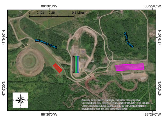
Figure 1.
The locations of the five soil pits at KRC are highlighted. Boxes show the area of the soil pits: Fine (red), Coarse (blue), Rink (green), Stability (purple), and 2NS (black).

Table 1.
Keweenaw Research Center (KRC) Soil Information. % Gravel, % Sand, % Fine, D10, D30, D60, Cu, Cc, and Unified Soil Classification for Soil (USCS) Classification.

Figure 2.
Overview flowchart of the laboratory study process from beginning to end.
2.1. Thermal Remote Sensing Background
The electromagnetic spectrum is a way of classifying different wavelengths of electromagnetic energy. The visible wavelength, the ones human eyes can distinguish, is between 350–750 nm. There are other wavelengths, both longer and shorter, such as radio waves (longer, less energy) to gamma rays (shorter, higher energy). Depending on the wavelength, the energy being projected onto the interest area can be reflected, transmitted, or absorbed. The short-wave infrared wavelengths are where one starts recording, not the reflected data, but rather the energy that was absorbed and then re-emitted later. This is called thermal remote sensing.
Thermal remote sensing is unique because since the energy being recorded by the camera has been re-emitted, the collected information provides subsurface characteristics. In contrast, with visible light, we only see the surface reflected color (such as red or blue) rather than the subsurface properties. The temperature of the material is recorded using thermal cameras.
2.2. Thermal Inertia/Apparent Thermal Inertia
Thermal inertia (TI) is a way to measure the potential for absorbing and storing heat in a material. Shown below is the equation for calculating the thermal inertia of a material, Equation (3) [33,34].
The values for thermal conductivity (k), bulk density (ρ), and specific heat (c) cannot be collected using remote sensing. Instead, we approximate TI by using the ATI, by using variables that can all be collected remotely (Equation (4)) [33]. This formula uses only the temperature change (∆T) of a material and the albedo (α), the overall average reflectance of a material in the 400–900 nm range. This value changes based on the smoothness or roughness of a material, as well as its color.
2.3. Lab Setup and Sensors
The soils were organized in the lab into five separate bins of approximately 2 × 2 × 1 ft. (length × width × height). Heat sources, two 500 W work lights, were then placed above each bin. The work lights were mounted on two horizontal metal poles, as shown in Figure 3. These heat sources were approximately 1 m above the soil surface to allow for full and even coverage of the exposed soil. This was done to provide the means of examining temperature change over time and allow enough distance above the soil to image the entire surface area without capturing the work lights in the thermal image.
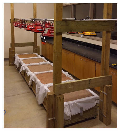
Figure 3.
Shows the lab setup of the 5 KRC soils. The soils in order from top left to bottom right: Fine, Coarse, Rink, Stability, and 2NS. Above each bin are two 500 W work lights.
Using a CR1000X data logger and CS615 water content reflectometers, the volumetric water content of the soils in each bin was collected. The CS615 and CR1000X full technical details can be located in the Campbell Scientifics manuals for each device [35,36]. The probes, 12 inches in length, were inserted at an angle to permit full submersion into the soil, ensuring we ranged from the surface to the bin’s base. The probes were removed after recording for 15 min, and soil was smoothed out.
The albedo was collected using an ASD Spectral Radiometer Handheld Pro, ranging from 350–900 nm. The range from 350–399 nm had a lot of noise, which made the data less reliable, so the 400–900 nm range was used to calculate the albedo of each soil [25]. To ensure that averaging was reliable, the reflectance values were collected at five different spots on the soil and tested 10 times. Full technical specifications are in the user manual [37].
The Humboldt GeoGauge was used on each soil to record stiffness [MN/m]. The GeoGauge does this by inducing small displacements on the soil using 25 steady-state frequencies, over the range of 100 to 196 Hz, and then averaging them to give the soil’s stiffness. The depth of this measurement is approximately 9–12 inches. With this range of frequencies, the measured stiffness is proportional to the shear modulus of the soil if one knows Poisson’s ratio [38].
Using a FLIR Duo R, the radiometrically calibrated temperatures were collected. This camera operates in the 7.5–13.5 μm wavelength range, and. the FLIR software automatically corrects the reflectance temperatures. This camera has a thermal sensor resolution of 160 × 120 pixels with a spectral band of 7.5–13.5 μm. The camera’s full technical aspects are in the FLIR Duo R manual [39].
2.4. Laboratory Testing Methodology
Initially, the volumetric water content was recorded by placing water content probes into each of the soil bins. These were then left to collect the average water content over 15-min. The probes were then removed and the soil smoothed out. A spectral radiometer was then used to collect samples from five different locations in each bin (each corner and the middle), and at each location the wavelengths were recorded from 350–900 nm. Each spot was tested 10 times at the same location. These values were then averaged over all tests and locations, for a total of 50 recordings per soil bin, which gave the single albedo value for each of the soils.
Next, the stiffness was recorded for each bin; the soil top was smoothed once again before thermal images were taken. The first thermal image was taken at hour 0 at a height of 1 m above the surface before the lights were turned on to get the starting temperature. Then, after every hour, a thermal image was captured for each bin throughout a four-hour time frame. The ATI was then calculated from the temperature change over the four hours and compared to the soil stiffness.
2.5. Machine Learning Background
Machine learning uses specific algorithms to mathematically predict the output (stiffness) by using different inputs (e.g., water content, ATI.). Various algorithms have different methodologies for predicting this outcome. The ones used in this study were linear, ridge [40,41,42], lasso [43,44], partial least squares [45], k nearest neighbors [2], and support vector machine regression [2,46,47,48,49]. Some of these algorithms were not scale-invariant so Box–Cox transformation, centering, and scaling were performed as an overall initial data preprocessing. A brief discussion of some of the regression methods used in this study is given below.
2.5.1. Linear Regression
Linear regression is the process of using a linear relationship between the predictors and the outcome while minimizing the sum of square error (SSE). Equation (5) shows the formula for SSE where n is the number of samples; yi is the observed value of the response variable, and ŷi is the predicted value for the response variable. This regression method is tuned by using different weight values as coefficients for each of the predictors to help enhance the prediction ability, in our case for soil stiffness. This is a very quick computational model that is highly interpretable, but it only performs well on data that have a linear relationship [40,41,42]. As linear regression creates coefficients that are unbiased when providing the lowest variance model, one can add bias to the coefficients to allow for penalized models such as ridge and lasso regression.
2.5.2. Ridge Regression
Ridge regression works by examining all of the input parameters and determines weights for each of those predictors’ importance by using the L2 regularization method, that is, the square of the coefficient weights [40,41,42]. Equation (6) show the ridge regression algorithm where λ is the cost parameter and βj is the weight for each individual predictor. It means that the value of those predictors which are less useful will be shrunk to smaller values, but not to zero. This algorithm still maintains all of the original predictors and does not perform feature selection. Tuning is performed by varying the cost (λ).
2.5.3. Lasso Regression
Lasso regression works in a similar manner, but instead of working with the L2 regularization, it works with the L1 regularization, that is, the absolute value of the weight of the coefficients [43,44]. Similarly, in the Equation (7) for lasso regression, λ is the cost parameter and βj is the weight for each individual predictor. This method will do feature reduction in situations where certain parameters may be of no use in the prediction process by setting their weight value to zero. Like that of ridge regression, tuning is performed over λ.
2.5.4. Partial Least Squares Regression
Partial least squares regression works by using latent variables and projecting the data into a new dimensional space. The latent variables are linear combinations of the predictors with different weights that explain the maximum variance of the data to better predict the response variable [45]. This methodology is similar to that of the principal component regression. Finding the optimal number of latent variables to use is the tuning parameter for this algorithm.
2.5.5. K Nearest Neighbors Regression
This algorithm, known as k nearest neighbors (KNN), works by taking a new data point and examining the surrounding data points that have the smallest distance from it. The number of nearest neighbors used is the tuning parameter for this model. One of the simplest ways to do this is to go over a range of values for k to see which has the best performance, as was the case for this work. Note, if you were to increase k to the number of sample points. you would end up simply going with the largest class in your data. More depth about this model is located in [2].
2.5.6. SVM Regression
SVM regression works by using a series of hyperplanes that act as a means to distinguish among the data. In a two-class linearly separable example, parallel hyperplanes were generated from the samples and the pair of samples that maximized the distance between the two classes were selected, the support vectors. The middle of the support vector is where a hyperplane is positioned perpendicular to both samples as a decision boundary between the two classes. The distance from this middle hyperplane to the nearest sample is called the margin. If the classes are not linearly separable then the kernel trick can be applied to map the dataset into a linearly separable space. A radial basis function kernel was used for this study. More information on this algorithm can be found in the following papers: [2,46,47,48,49].
3. Results
Results from the albedo found that each soil has a unique albedo value, but sometimes close to one another as shown in Table 2. This makes sense since the albedo is the average reflectance value in the visible-NIR spectrum, and each soil type is a different shade of color. This was evident in visual observation as seen previously in Figure 2. Values for GeoGauge stiffness also had specific ranges but varied based on the water content; see Table 3. The % moisture content ranges generally go from 2 to 4%, but for “Stability” one of the tests had a larger moisture content of 8%, increasing its average higher.
Table 2.
Table of albedo mean values and ranges for each soil.
Table 3.
Table of stiffness (MN/m) and ATI ranges and means for each soil. ATI values are taken after 3 h of heating.
The temperature change of the soil over time had an overall increasing effect but began to level off after about 2 h. The soils still changed uniquely for the next hour, but at hour 4, the different soils hit their threshold and began to converge, as seen in Figure 4. The 3 h mark is approximately where the diurnal cycle temperature change would be; however, testing was done to 4 h to see where the soils’ temperatures would begin to converge (or rather become oversaturated). Correspondingly, we noticed the ATI of the soils decreasing over time and following a similar plateau shape; see Figure 5. To maximize the performance among the machine learning models, the ATI at the 3 h mark was used as it provided the best distinction between the five soil types. Recalling Equation (4), the ATI showed a roughly mirror image to that of the temperature change because the larger the temperature change, the smaller the ATI value, as seen in Figure 5.
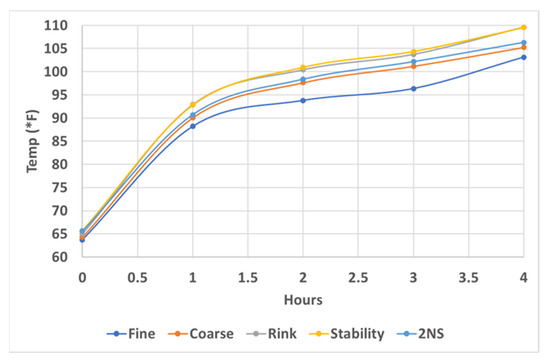
Figure 4.
Plot of the average change in temperature over time for each of the five soils.
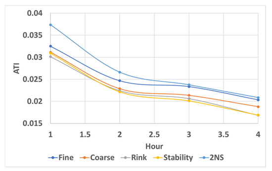
Figure 5.
Plot of the average change in ATI over time for each of the five soils.
The data were then organized and loaded into Python for processing. Box plots of the samples’ stiffness values are shown below in Figure 6. When examining all the samples, one saw that there was a range of strength values that came in a variety of conditions. It was also apparent that a simple linear correlation to either ATI (Figure 7) or moisture content (Figure 8) alone was not possible, further validating the need to build a more complex model with multiple predictors.
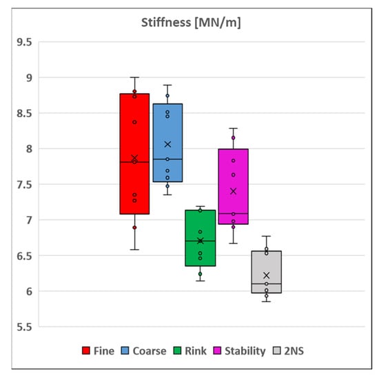
Figure 6.
Box plot of the soil stiffness values [MN/m] for each of the individual soil types from all laboratory trials.
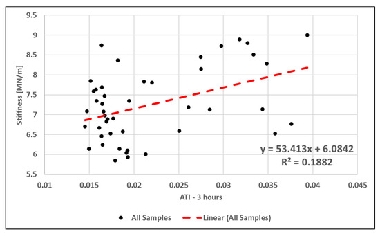
Figure 7.
Plot of all the samples Stiffness (MN/m) verses ATI.
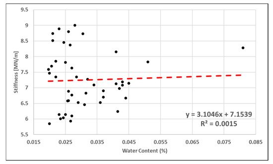
Figure 8.
Plot of all the samples Stiffness [MN/m] verses Water Content [%].
Initial data preprocessing included Box–Cox transformation, centering, and scaling of the data. Some of the algorithms are scale-invariant; that is, they are affected by the numerical values, which means a predictor with a value of 10 will have a smaller impact than a predictor with a value of 100. The total sample size was gathered from 9 laboratory tests for each of the 5 soil types, leading to 45 observations. Data used an 80/20 (train/test) split with random sampling (even distribution among the soil types). K-fold cross-validation was applied when tuning the training data parameters, and then the best models (models with optimal tuning parameters) were run on the test set.
Different sets of predictors were examined to find the minimum number of variables needed while maintaining good predictive capability within the model. Trials were run solely to examine the correlation between soil stiffness (response), the % water content and the ATI for 3 h for the first group. The second group of predictors was conducted with % water content, ATI 3 h, and the values for calculating the ATI (temperature at 0 h and 3 h, and albedo). Thirdly, the addition of soil information, or rather the use of dummy variables to identify the soil type, was added to each of the prior-mentioned predictor groups for testing. Initial results for the different models are shown in the table below. The best fit for the models is shown in Figure 9 using ATI (3 h), % water content, and soil type information using the KNN model.
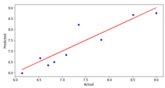
Figure 9.
Actual versus predicted outcome using ATI (3 h), % water content, and soil type information from the KNN model.
4. Discussion
Table 4 displays the values for each of the classifiers using different predictor sets and shows % water content and ATI (3 h) alone did not give enough information to estimate soil stiffness accurately. Adding in the predictors in group 2 (% water content, ATI (3 h), temperature at 0 and 3 h, and albedo) gave enough information for the algorithms to predict soil stiffness values somewhat. We still saw an increase in information when we added dummy variables to describe the soil type. With the additional soil type information, we improved the models in such a way that only the % water content and ATI (3 h) provided the best results for prediction accuracy.
Table 4.
Table of Prediction accuracy (R2) and Root Mean Squared Error (RMSE) for each of the regression models implemented on each predictor set.
If one is using only the thermal imagery process, the best methodology would therefore be to use group 2’s set of predictors: % water content, ATI (3 h), temperature at 0 and 3 h and the albedo. If the soil type under examination is known the model dimensions can be lowered to % water content, ATI (3 h), and soil type.
The success rate of these algorithms shows that using only ATI and soil moisture to predict the soil stiffness yields an R2 value of 0.381. Adding in the predictors’ additional information to calculate the ATI enhanced the predictive capability by giving an R2 value of 0.661. Finally, additional information about the soil type being examined adds significant enhancement to these algorithms’ predictive ability for the original two predictor sets: R2 = 0.824 and R2 = 0.755, respectively. The ATI, % water content, and the soil information yielded the best R2 and lowest RMSE value using KNN, thereby making this the optimal choice of parameters and model. Using the KNN model, we quantitatively predicted the soil stiffness reasonably well by using only the ATI after 3 h, % water content, and soil type information. When looking at similar work, the conclusions are mostly qualitative [9]. Gonzalez and his group stated which remote-controlled car could cross a select few, very different terrains the fastest without getting stuck.
A significant limitation of this study is the sample size. Its focus was to demonstrate the applicability of this approach in a controlled lab environment. Another limitation is that we only examined five soil types. We are in the process of expanding this work to the field and other soil types and will build the machine-learning model for the field with a larger database.
It is important to note that this study showed the applicability of the approach in a controlled laboratory environment. When this approach is performed in the field, multiple inputs may differ, ranging from the mixing of soils, changes in water content values, and sensor/scan area resolutions. While one cannot reasonably expect there to be identical conditions every time a field site is visited, the approach followed in the lab will be applied in the field.
5. Conclusions
This study showed that the use of ATI with the addition of moisture content and soil information provided a usable methodology for estimating soil stiffness. A comparison of different machine-learning algorithms showed that KNN was the best predictive algorithm for this lab study when using the previously mentioned predictor variables (R2 = 0.824). This KNN model provided a fairly accurate soil stiffness estimation tool that required few inputs and allowed for implementation over an image area. Using KNN with albedo, temperature at 0 and 3 h), ATI (3 h), and % moisture content, but no soil information, gave only a moderate predictive ability (R2 = 0.66). This should be used only when no soil information is available as a rough estimation.
Present methodologies of in situ measurements can be both costly and difficult to obtain to characterize terrain strength. In contrast, the means of predicting soil stiffness through ATI is a safer, faster means to collect data. The KNN model provided a method to estimate the stiffness of the five soils provided by the Keweenaw Research Center’s mobility testing tracks.
By using only remotely sensed data, the thermal images, % water content, and soil stiffness can be estimated. This means a UAV or satellite could fly over an area and take three images of interest without someone going there. With relatively inexpensive tools, one could characterize the terrain strength, and remote sensing is a better means of collection because one is no longer limited to point location collections; instead, an entire area can be estimated within the images. Adding additional information about what soil type is being examined enhances predictions. The limitations would be the resolution of the thermal camera, the sensor recording the albedo (hyperspectral camera), and the need to wait for a large enough temperature change to occur. The ability of the proposed approach for other soil types such as silt, clay, loam, and peat need to be tested.
Landsat 8 and Landsat 9 satellites already have bands available to capture and calculate the ATI of an area. The resolution of these satellites––30 m for capturing the albedo (bands 1–5) and 100 m for the thermal bands (bands 10–11)––would need to be examined to see if this model would still hold at this resolution. To validate the results, one would need to know the soil strength for a specified area of 100 m of thermal imagery. If one were to meet these conditions and establish a working model, a variety of scenarios could be examined across the world in various conditions and for a variety of soil types using these satellites. One could even look to using this approach on a smaller scale (higher resolution) to estimate the strength of an area and then compare the results with the satellite imagery to help better validate the results of the lower-resolution sensors. If this is not possible, ground-control points or specific areas with known soil strength values can be used to train and build the model with the understanding that some level of uncertainty may be added because the known soil strength of an area could be smaller than the resolution of sensor.
In future research, we hope to examine soil types beyond the five examined here, including those that have of organics present. The use of drones and satellites, which have a larger area coverage and different spatial resolutions is of great interest for seeing how the model holds up at the various scales and heights. All our current sensors are UAS mountable and can therefore be taken out into the field for testing at various heights and resolutions. This also adds more real-world data scenarios and larger sample sizes. The use of hyperspectral data could add extra information to classify the soil type, instead of using dummy variables, and improve the prediction accuracy of these models. Lastly, collecting a much larger sample size could lead to using deep-learning methods that would not only to check the accuracy of our current models, but also possibly improve our predictive capabilities, especially when we begin to examine more soil types and conditions.
Author Contributions
J.E., T.O. and P.J. conceived and designed the experiments; J.E. and T.O. performed the experiments; J.E, T.O. and P.J. analyzed the data; J.E. and T.O. wrote the original draft preparation; J.E, T.O., P.J. and R.A. contributed to writing—review and editing. All authors have read and agreed to the published version of the manuscript.
Funding
This research was funded by the University of Michigan’s Automotive Research Center (ARC), the U.S. Army Combat Capabilities Development Command Ground Vehicle Systems Center (CCDC-GVSC, formerly TARDEC), and Michigan Technological University (MTU).
Acknowledgments
We would like to acknowledge the technical and financial support of the Automotive Research Center (ARC) in accordance with Cooperative Agreement W56HZV-19-2-0001 U.S. Army Ground Vehicle Systems Center (GVSC) Warren, MI. We would also like to thank Michigan Technological University (MTU) for helping to fund this research and the Keweenaw Research Center (KRC) for providing the logistics for data collection.
Conflicts of Interest
The authors declare no conflict of interest.
Disclaimer
DISTRIBUTION A. Approved for public release; distribution unlimited. OSPEC #5204.
References
- McCullough, D.M.; Jayakumar, D.P.; Dasch, D.J.; Gorsich, D.D. Developing the Next Generation NATO Reference Mobility Model. In Proceedings of the 2016 Ground Vehicle Systems Engineering and Technology Symposium (GVSETS), Novi, MI, USA, 2–4 August 2016. [Google Scholar]
- Mechergui, D.; Jayakumar, P. Efficient generation of accurate mobility maps using machine learning algorithms. J. Terramech. 2020, 88, 53–63. [Google Scholar] [CrossRef]
- Pandey, V.; Bos, J.P.; Ewing, J.; Kysar, S.; Oommen, T.; Jayakumar, P.; Gorsich, D. Decision-Making for Autonomous Mobility Using Remotely Sensed Terrain Parameters in Off-Road Environments; SAE Technical: Warrendale, PA, USA, 2021. [Google Scholar]
- Okello, J.A. A Review of Soil Strength Measurement Techniques for Prediction of Terrain Vehicle Performance. J. Agric. Eng. Res. 1991, 50, 129–155. [Google Scholar] [CrossRef]
- Shoop, S.A. Terrain Characterization for Trafficability; CRREL Report 93-6; US Army Corps of Engineers Cold Regions Research & Engineering Laboratory: Hanover, NH, USA, 1993. [Google Scholar]
- Li, H.; Chen, L.; Li, F.; Huang, M. Ship detection and tracking method for satellite video based on multiscale saliency and surrounding contrast analysis. J. Appl. Remote Sens. 2019, 13. [Google Scholar] [CrossRef]
- Bialas, J.; Oommen, T.; Havens, T.C. Optimal segmentation of high spatial resolution images for the classification of buildings using random forests. Int. J. Appl. Earth Obs. Geoinf. 2019, 82, 101895. [Google Scholar] [CrossRef]
- Samui, P.; Gowda, P.H.; Oommen, T.; Howell, T.A.; Marek, T.H.; Porter, D.O. Statistical learning algorithms for identifying contrasting tillage practices with Landsat Thematic Mapper data. Int. J. Remote Sens. 2012, 33, 5732–5745. [Google Scholar] [CrossRef]
- González, R.; López, A.; Iagnemma, K. Thermal vision, moisture content, and vegetation in the context of off-road mobile robots. J. Terramech. 2017, 70, 35–48. [Google Scholar] [CrossRef]
- Yang, L.; Wang, L.; Huang, J.; Mansaray, L.R.; Mijiti, R. Monitoring policy-driven crop area adjustments in northeast China using Landsat-8 imagery. Int. J. Appl. Earth Obs. Geoinf. 2019, 82. [Google Scholar] [CrossRef]
- Waldner, F.; Diakogiannis, F.I. Deep learning on edge: Extracting field boundaries from satellite images with a convolutional neural network. Remote Sens. Environ. 2020, 245. [Google Scholar] [CrossRef]
- Hossain, M.D.; Chen, D. Segmentation for Object-Based Image Analysis (OBIA): A review of algorithms and challenges from remote sensing perspective. ISPRS J. Photogramm. Remote Sens. 2019, 150, 115–134. [Google Scholar] [CrossRef]
- Minasny, B.; McBratney, A.B. Digital soil mapping: A brief history and some lessons. Geoderma 2016, 264, 301–311. [Google Scholar] [CrossRef]
- Yang, J.; Li, P.; He, Y. A multi-band approach to unsupervised scale parameter selection for multi-scale image segmentation. ISPRS J. Photogramm. Remote Sens. 2014, 94, 13–24. [Google Scholar] [CrossRef]
- Stark, N.; McNinch, J.; Wadman, H.; Graber, H.C.; Albatal, A.; Mallas, P.A. Friction angles at sandy beaches from remote imagery. Géotechnique Lett. 2017, 7, 292–297. [Google Scholar] [CrossRef]
- Strojnik, M.; Merola, P.; Allegrini, A.; Guglietta, D.; Sampieri, S. Buried archaeological structures detection using MIVIS hyperspectral airborne data. In Proceedings of the Infrared Spaceborne Remote Sensing XIV, San Diego, CA, USA, 13–17 August 2006. [Google Scholar]
- Ewing, J.; Oommen, T.; Jayakumar, P.; Alger, R. Utilizing Hyperspectral Remote Sensing for Soil Gradation. Remote Sens. 2020, 12, 3312. [Google Scholar] [CrossRef]
- Schulz, K.; Michel, U.; Geller, C. A comprehensive land cover classification approach for the development of wildfire fuels layers. In Proceedings of the Earth Resources and Environmental Remote Sensing/GIS Applications IX, Berlin, Germany, 11–13 September 2018. [Google Scholar]
- Valero, M.M.; Rios, O.; Mata, C.; Pastor, E.; Planas, E. GIS-based integration of spatial and remote sensing data for wildfire monitoring. In Proceedings of the Earth Resources and Environmental Remote Sensing/GIS Applications IX, Berlin, Germany, 11–13 September 2018. [Google Scholar]
- Kumar, C.; Chatterjee, S.; Oommen, T.; Guha, A. Automated lithological mapping by integrating spectral enhancement techniques and machine learning algorithms using AVIRIS-NG hyperspectral data in Gold-bearing granite-greenstone rocks in Hutti, India. Int. J. Appl. Earth Obs. Geoinf. 2020, 86. [Google Scholar] [CrossRef]
- Kumar, C.; Chatterjee, S.; Oommen, T. Mapping hydrothermal alteration minerals using high-resolution AVIRIS-NG hyperspectral data in the Hutti-Maski gold deposit area, India. Int. J. Remote Sens. 2019, 41, 794–812. [Google Scholar] [CrossRef]
- Shaw, G.A.; Burke, H.-H.K. Spectral Imaging for Remote Sensing. Linc. Lab. J. 2003, 14, 3–28. [Google Scholar]
- Bishop, S.S.; Isaacs, J.C.; Gagnon, M.-A.; Lagueux, P.; Gagnon, J.-P.; Savary, S.; Tremblay, P.; Farley, V.; Guyot, É.; Chamberland, M. Airborne thermal infrared hyperspectral imaging of buried objects. In Proceedings of the Detection and Sensing of Mines, Explosive Objects, and Obscured Targets XX, Baltimore, ML, USA, 20–23 April 2015. [Google Scholar]
- Bowman, A.P.; Winter, E.M.; Stocker, A.D.; Lucey, P.G. Hyperspectral Infrared Techniques for Buried Landmine Detection. In Proceedings of the 1998 Second International Conference on the Detection of Abandoned Land Mines, Edinburgh, UK, 12–14 October 1998; pp. 129–133. [Google Scholar]
- Zwissler, B.; Oommen, T.; Vitton, S.; Seagren, E.A. Thermal Remote Sensing For Moisture Content Monitoring of Mine Tailings: Laboratory Study. Environ. Eng. Geosci. 2017, 23, 299–312. [Google Scholar] [CrossRef]
- Badarinath, K.V.S.; Chand, T.R.K. Analysis Of Apparent Thermal Inertia Over Different Land Use/Land Cover Types Using Envisat Aatsr Data. J. Indian Soc. Remote Sens. 2007, 35, 185–191. [Google Scholar] [CrossRef]
- Lei, S.-g.; Bian, Z.-f.; Daniels, J.L.; Liu, D.-l. Improved spatial resolution in soil moisture retrieval at arid mining area using Apparent Thermal Inertia. Trans. Nonferrous Met. Soc. China 2014, 24, 1866–1873. [Google Scholar] [CrossRef]
- Scheidt, S.; Ramsey, M.; Lancaster, N. Determining soil moisture and sediment availability at White Sands Dune Field, New Mexico, from Apparent Thermal Inertia data. J. Geophys. Res. Earth Surf. 2010, 115. [Google Scholar] [CrossRef]
- Sohrabinia, M.; Rack, W.; Zawar-Reza, P. Soil moisture derived using two Apparent Thermal Inertia functions over Canterbury, New Zealand. J. Appl. Remote Sens. 2014, 8. [Google Scholar] [CrossRef]
- Taktikou, E.; Bourazanis, G.; Papaioannou, G.; Kerkides, P. Prediction of Soil Moisture from Remote Sensing Data. Procedia Eng. 2016, 162, 309–316. [Google Scholar] [CrossRef][Green Version]
- Gao, Y.; Spiteri, C.; Li, C.-L.; Zheng, Y.-C. Lunar soil strength estimation based on Chang’E-3 images. Adv. Space Res. 2016, 58, 1893–1899. [Google Scholar] [CrossRef]
- ASTM. Standard Practice for Classification of Soils for Engineering Purposes (Unified Soil Classification System); D2487–17; ASTM International: West Conshohocken, PA, USA, 2019. [Google Scholar] [CrossRef]
- Minacapilli, M.; Cammalleri, C.; Ciraolo, G.; D’Asaro, F.; Iovino, M.; Maltese, A. Thermal Inertia Modeling for Soil Surface Water Content Estimation: A Laboratory Experiment. Soil Sci. Soc. Am. J. 2012, 76, 92–100. [Google Scholar] [CrossRef]
- Jensen, J.R. Remote Sensing of the Environment: An Earth Resource Perspectie 2/e; Pearson Education: New Delhi, India, 2009. [Google Scholar]
- Campbell Scientific, I. CR1000X. Product Manual 2018. Available online: https://www.campbellsci.com/cr1000x (accessed on 11 June 2021).
- Campbell Scientific, I. CS615–Water Content Reflectometer. 1996. Available online: https://s.campbellsci.com/documents/us/manuals/cs615.pdf (accessed on 11 June 2021).
- Analytical Spectral Devices, I. FieldSpec HandHeld Manual. 2002. Available online: https://www.malvernpanalytical.com/en/support/product-support/asd-range/fieldspec-range/handheld-2-hand-held-vnir-spectroradiometer#manuals (accessed on 11 June 2021).
- Humboldt. H-4140–GeoGauge. 2014. Available online: https://www.humboldtmfg.com/geogauge.html (accessed on 11 June 2021).
- FLIR. flir-duo. User-Guide. 2016. Available online: https://www.flir.com/support/products/duo-r/#Overview (accessed on 11 June 2021).
- Guilkey, D.K.; Murphy, J.L. Directed Ridge Regression Techniques in Cases of Multicollinearity. J. Am. Stat. Assoc. 1975, 70, 769–775. [Google Scholar] [CrossRef]
- Marquardt, D.W.; Snee, R.D. Ridge Regression in Practice. Am. Stat. 1975, 29, 3–20. [Google Scholar] [CrossRef]
- Hoerl, A.E.; Kennard, R.W. Ridge Regression: Biased Estimation for Nonorthogonal Problems. Technometrics 1970, 12, 55–67. [Google Scholar] [CrossRef]
- Tibshirani, R.; Johnstone, I.; Hastie, T.; Efron, B. Least angle regression. Ann. Stat. 2004, 32, 407–499. [Google Scholar] [CrossRef]
- Tibshirani, R. Regression Shrinkage and Selection Via the Lasso. J. R. Stat. Society. Ser. B Methodol. 1996, 58, 267–288. [Google Scholar] [CrossRef]
- Geladi, P.; Kowalski, B.R. Partial least-squares regression: A tutorial. Anal. Chim. Acta 1986, 185, 1–17. [Google Scholar] [CrossRef]
- Burges, C.J.C. A Tutorial On Support Vector Machines for Pattern Recognition. Data Min. Knowl. Discov. 1998, 2, 121–167. [Google Scholar] [CrossRef]
- Cristianini, N. An Introduction to Support Vector Machines and Other Kernel-Based Learning Methods; Cambridge University Press: Cambridge, UK, 2000. [Google Scholar]
- Melgani, F.; Bruzzone, L. Classification of hyperspectral remote sensing images with support vector machines. IEEE Trans. Geosci. Remote Sens. 2004, 42, 1778–1790. [Google Scholar] [CrossRef]
- Mũnoz-Marí, J.; Bovolo, F.; Gómez-Chova, L.; Bruzzone, L.; Camp-Valls, G. Semisupervised One-Class Support Vector Machines for Classification of Remote Sensing Data. IEEE Trans. Geosci. Remote Sens. 2010, 48, 3188–3197. [Google Scholar] [CrossRef]
Publisher’s Note: MDPI stays neutral with regard to jurisdictional claims in published maps and institutional affiliations. |
© 2021 by the authors. Licensee MDPI, Basel, Switzerland. This article is an open access article distributed under the terms and conditions of the Creative Commons Attribution (CC BY) license (https://creativecommons.org/licenses/by/4.0/).