1. Introduction
The realization and maintenance of a terrestrial reference frame (TRF) is foundational for the understanding and investigation of the linear and nonlinear time variations of the solid earth’s shape caused by various geophysical processes, such as plate tectonics [
1,
2,
3], glacial isostatic adjustment [
4,
5], and large scale surface mass (atmosphere, snow, glacier, soil moisture, and ground water storage) variations [
6,
7], and sea level rise [
8,
9,
10,
11]. The TRF also plays a critical role as the reference in operational geodesy applications, such as precise point positioning, precise orbit determination, and natural hazard monitoring. High accuracy, consistency, and long-term stability of a TRF are required for geophysical and geodetic applications, demanding that the accuracy and stability of the TRF to be at the 1 mm and 0.1 mm/yr level [
8,
12].
The most recent realizations with the combination strategy and physical model enhancement are ITRF2014 [
13], DTRF2014 [
14], and JTRF2014 [
15], respectively. All three realizations are computed on the basis of the data from four space geodetic techniques [
16], including Global Navigation Satellite System (GNSS), Doppler Orbitography and Radiopositioning integrated by Satellite (DORIS), Satellite Laser Ranging (SLR), and Very Long Baseline Interferometry (VLBI). As no single space geodetic technique is able to provide the full reference frame-defining parameters, the strengths of the four contributing space geodetic techniques are integrated, and their weaknesses and systematic errors are mitigated.
Although identical input data were used, the three realized TRFs are defined in different conceptions [
16]. While ITRF2014 and DTRF2014 are based on a piecewise linear motion model of global distributed stations with positions at a reference epoch and velocities, JTRF2014 is a time series-based frame. The two secular solutions, ITRF2014 and DTRF2014, are established following a two-step procedure: (1) stacking the individual time series to estimate a long-term solution for each space technique; and (2) combining the four long-term solutions together by means of local ties at co-location sites.
ITRF2014 and DTRF2014 are computed by the combination of solutions and normal equations, respectively [
14], and they differ from the modeling of non-linear station motions: the sites deformation after major earthquakes are described by post-seismic deformation (PSD) models in the ITRF2014, while the DTRF2014 uses piece-wise linear models to represent the earthquake-affected station positions. Furthermore, the atmospheric and hydrological non-tidal loading (NTL) was applied within the DTRF2014 computation, while seasonal (annual and semiannual) signals of station positions were estimated within the ITRF2014 computation. The averaging strategies for scale are the arithmetic mean and the weighted average of VLBI and SLR for the ITRF2014 and the DTRF2014. Different combination strategies and combination models of local tie techniques at co-location sites used by the realized TRFs may lead to differences in the reference-frame-defining parameters.
Owning to its large number and the extensive distribution of geodetic stations on the ground, the International GNSS Service (IGS) plays a crucial role in the realization and densification of TRFs along with its continuous improvement in data precision. The orientation definition of a TRF generally relies on a well-distributed ground network, where other space techniques are inaccessible due to limited ground sites and distributions. Furthermore, GNSS sites act as a connector at co-location sites when combining the four contributing techniques, which benefit from the precise positions and lower-cost construction of sites.
In addition to the essential status in the realization of International Terrestrial Reference System (ITRS), the IGS maintains GNSS-based TRFs, such as IGb08 and IGS14, which are used as the reference datum for precise orbit determination and deformation monitoring etc. As the real-time updating of the IGS datum, non-linear variations, including real geophysical crustal motions, artificial variations, and unexplained variations [
17], are contained in the time series of station positions, IGS solutions are superior to the secular frames with only linear information included. Moreover, position discontinuities induced by equipment changes or earthquakes, etc. are properly handled in the IGS solutions.
The determination of a new TRF involves great efforts of data analysis for large amount of historical data and is normally updated every 5–6 years. During the period between the generation of the up-to-date ITRS realization and its next release, IGS solutions can provide ultimate accurate positions of ground sites based on the minimal constraints applied to a subset of core stations. The IG2 solutions are based on the second IGS reprocessing campaign (repro2) to provide homogeneous IGS inputs to the three mentioned TRF realizations [
18,
19]. GNSS data spanning from 1994 to 2014 were reanalyzed by nine different Analysis Centers (ACs) using the latest available models and methodology.
Since geocenter motions estimated from the GNSS technique are biased by orbit modeling errors and severe correlation with other parameters (like clock offsets and tropospheric parameters) [
20,
21,
22], the origin of the final combined solution is aligned to IGb08 with minimum constraints (no-net-translation, NNT) applied to a subset of core stations [
23]; the orientation is aligned to IGb08 with no-net-rotation (NNR) applied to the same core network; and the scale is defined by using the igs08.atx based satellite PCO values [
18,
24]. The IGS solutions are based on the IGb08 frame before 28 February 2017, and then they are aligned to the IGS14 frame until 16 May 2020 and the IGb14 frame thereafter.
IGS14 and IGb14 were defined similarly with origin, orientation, and scale consistent with ITRF2014, except that nine additional stations and five more years of data were involved for the construction of the IGb14 frame (
https://lists.igs.org/pipermail/igsmail/2020/007917.html) (accessed on 28 May 2021). A third reprocessing campaign of GNSS/DORIS/SLR/VLBI observations has been performing so as to provide the new input to the upcoming new TRF release. For the new TRF release, the additional 6 years of observations, new sites and local ties will be included, so as to improve its overall performance.
With regard to the comparison of TRF realizations, the studies of Abbondanza et al. (2020) [
25] indicated that the level of long-term consistency between the three products is in the order of 0.18 mm/yr. The results of Angermann et al. (2020) [
16] revealed (1) almost the same accuracy level for ITRF2014, DTRF2014, and JTRF2014, within which, the best results were obtained from JTRF2014 and DTRF2014+NTL, by performing a comparison of the three latest realizations using Precise Orbit Determination (POD) and SLR data; (2) the geodetic datum (origin, scale, and orientation) between the two long-term realizations, the ITRF2014 and DTRF2014, agreed within 5–6 mm by applying 14-parameter Helmert transformations individually for the four different space techniques.
Dach et al. (2016) [
26] suggested that the differences between the most recent ITRF realizations were smaller than the effects from the distortion introduced into the solution by forcing the center of mass into the origin, while the studies in Dach et al. (2017) [
27] indicated that the differences between the ITRF realizations were smaller than the effects from orbit modeling errors of GNSS satellites and station-/satellite-specific effect introduced by the SLR technology.
Due to the model deficiency, ITRF2014, DTRF2014, and JTRF2014 unavoidably exhibit accuracy degradation with time evolution. In this paper, we use the continuously observed GNSS frame solutions, i.e., the IG2 solutions from January 1995 to January 2015 and the IGS solutions from February 2015 to July 2020 as reference benchmarks to study the signals in the three realizations and their performance in frame prediction. The Helmert transformation approach and related parameters are used to study the discrepancies and consistencies between the IGS solutions and up-to-date TRF realizations. In
Section 2, the selected stations used to perform similarity transformation are illustrated. Then, the IGS solutions are compared to ITRF2014, DTRF2014, and JTRF2014 and their predictions in the following sections.
2. Selected GNSS Station Networks
As an indispensable component of TRS realizations, IG2 reveals its predominant status in time series combinations of global frames especially due to the extensive distribution of ground stations and the accurate determination of station positions. The IGS/IG2 solutions combine daily solutions from different GNSS Analysis Centers based on diverged network geometry and their own processing strategies. All the available signals are combined, and spurious signal are mitigated in the IG2 time series through the advantageous combination strategies used by IGS. The daily origin and orientation are aligned to IGb08/IGS14 by NNT and NNR constraints, and the two IGS reference frames are extracted from the linear frame ITRF2008 and ITRF2014, respectively.
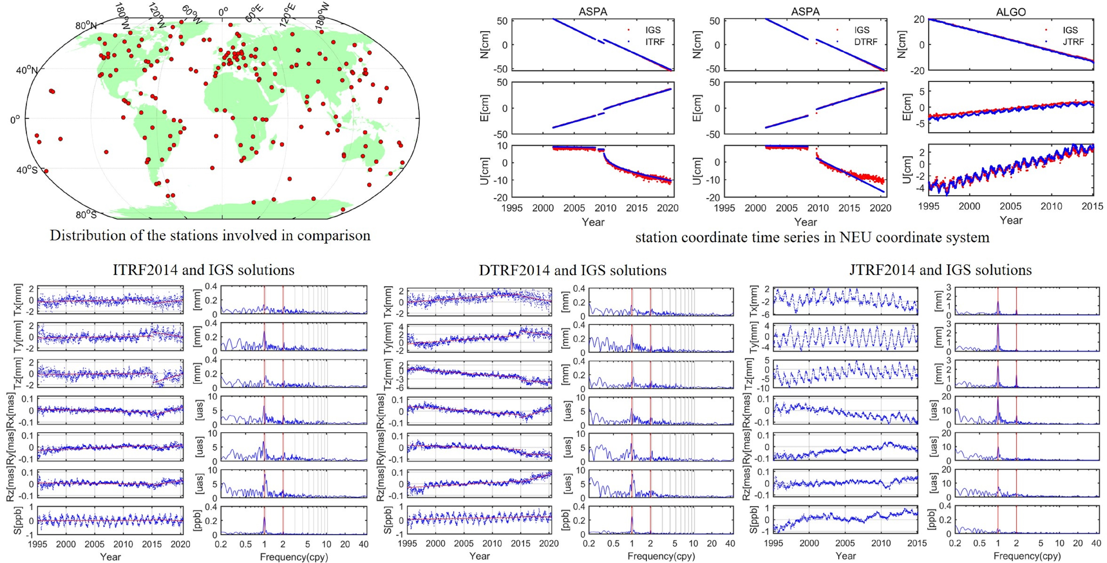
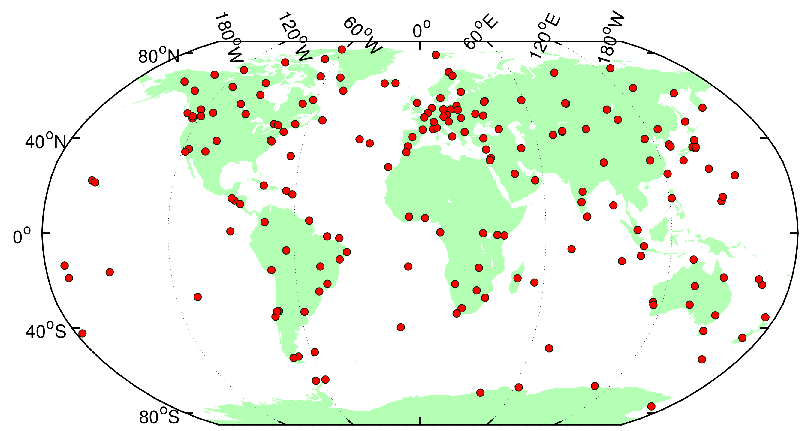
Helmert transformation is a typical method for reference frame analysis, and its parameter estimates may be affected by the network distribution. A stable and well distributed network is selected with 165 ground stations, which is displayed in
Figure 1, and the number variation of the selected stations involved in the comparisons over time is displayed in
Figure 2. The selection criteria contained two main points: continuity and stability of the stations participating in the daily solutions, where all the stations contain at least a data span of a 2-year consecutive period.
3. Comparison between ITRF2014 and IGS
ITRF2014 is a superior release compared to past ITRS realizations with two innovations implemented in the construction of the ITRF2014: First, post-seismic deformation (PSD) models along with linear station motions are provided for the stations affected by major earthquakes; Second, seasonal signals (annual and semi-annual) are estimated at the stacking step for the purpose of acquiring more precise velocities of ground stations. As it precisely models the actual trajectories of station position time series, ITRF2014 was demonstrated to be a more robust secular frame.
In this section, IG2 daily solutions from January 1995 to January 2015 and IGS solutions from February 2015 to July 2020 were selected to compare with the ITRF2014 positions of the selected stations, where the station coordinates of ITRF2014 after January 2015 were from the prediction based on ITRF models.
In the following, both IG2 and IGS are uniformly called IGS. The IGS and ITRF2014 station coordinate time series for ALBH and MIZU are plotted in
Figure 3. The site ALBH experienced an abrupt break on 15 September 2015 due to an antenna change, while the corresponding coordinate corrections were not possible to be derived from the ITRF2014 model. The site MIZU suffered increasing position errors in the ITRF2014 models due to inaccurate position prediction of the PSD model after January 2015. The accuracy of the ITRF2014 became worse when the number of sites, such as ALBH and MIZU, reached a certain amount.
In order to further assess the discrepancies between the two linear frames, a Helmert transformation was performed between them. In the Helmert transformation processing, the outlier rejection thresholds were 10, 10, and 30 mm in the N, E, and U components, respectively [
28].
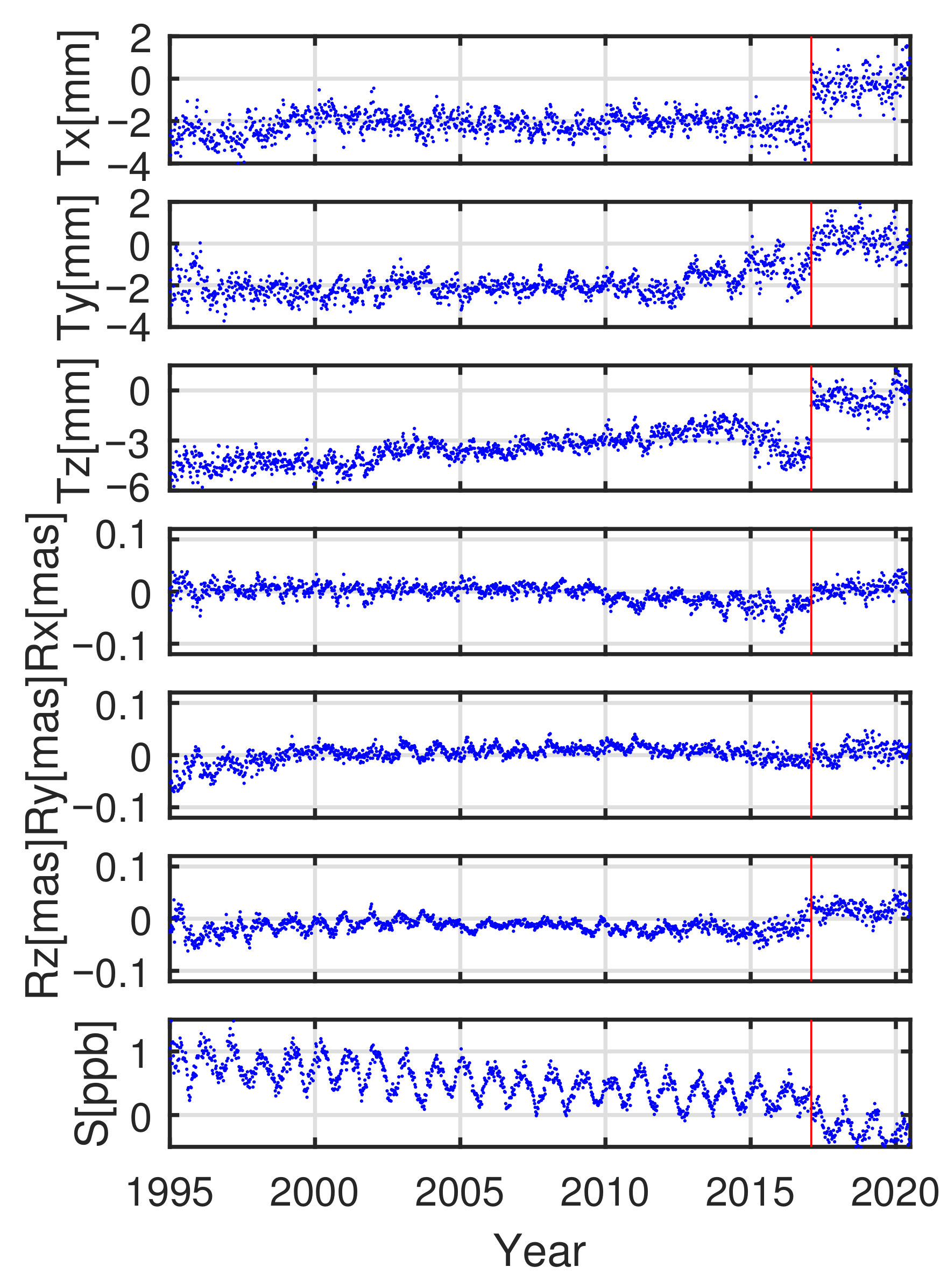
Figure 4 displays the translation, rotation, and scale time series estimated between the ITRF2014 and IGS solutions. The discontinuity that occurs in February 2017 is due to the fact that the IGS daily solutions were switched from IGS realizations of ITRF2008 (i.e., IGb08) to ITRF2014 (i.e., IGS14) on 28 February 2017.
Non-zero constant offsets of the X, Y components of −2.16 ± 0.51 and −1.97 ± 0.59 mm were observed in the time series before 28 February 2017. The slope 0.12 mm/yr and −0.03 ppb/yr were found in the Z component of the translation and scale time series, which is coincident to the transformation parameters from ITRF2014 to ITRF2008 [
13]. The origin and orientation of IGS were aligned to the IGb08 before 28 February 2017, and the scale of IGS was determined by using the igs08.atx [
18].
Both the drift of the Z component translation time series and scale offsets suggest precision improvements coming from the contributing reprocessed data because of the corresponding improved technique-specific analysis strategies in ITRF2014. The rotation parameters in all components with negligible offsets and temporal variations before 14 February 2015 demonstrated excellent agreement of orientation between the IGS solutions and ITRF2014 due to the NNR constraint applied to successive ITRFs. Greater biases in the period from 1995 to 1998 may be caused by the poor geometry distribution of usable GNSS stations selected for the minimum constraints in the IGS daily solutions.
To obtain homogeneous results of the Helmert transformation comparison, we corrected the IGS solutions before 29 February 2017 to be uniform with the IGS14 using the two-step transformation recommended by Rebischung et al. 2012 [
29]. In addition, offsets generated from the long-term scale rate difference of 0.026 ppb/yr between the ITRF2014 and IGS14-based IGS solutions after January 2017 were subtracted to search for completed uniformity [
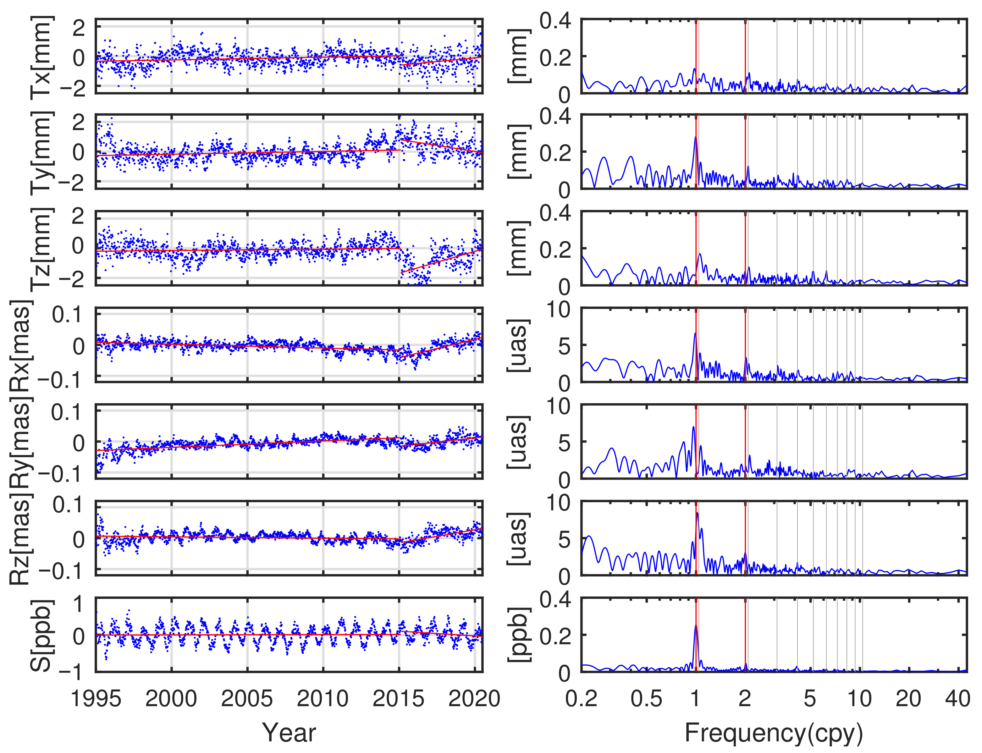
30]. The transformation parameters after the frame alignment and their amplitude spectrum are displayed in
Figure 5. The time series of the seven transformation parameters became more consistent after the correction especially for the translation and scale parameters. Remaining discrepancies still appeared in the translation time series from October 2012 to January 2017, in which the offsets could be up to 1.8 and 2.0 mm in the X and Y components, respectively. This may be caused by the geometry degradation of the IGb08 core network during that period.
To study the degradation degree of ITRF2014, the time series of the transformation parameters were divided into two sections, where the first section, from January 1995 to February 2015, is the ITRF2014 determination period, and the section from February 2015 until July 2020 is the ITRF2014 extrapolating (prediction) period. The drifts and standard deviations of the transformation parameter time series were estimated between ITRF2014, and the corrected IGS solutions of the two sections are provided in
Table 1.
Compared to the first section, the fitting drifts of the second sections showed non-negligible trends, especially for the rotation parameters with drifts of 11.9, 5.5, and 8.4 μas/yr in the X, Y, and Z components, respectively, which reflects the accuracy degradation embodied in the orientation of ITRF2014. Apparent drifts were also presented in the Y and Z translation parameters. A rate of −0.038 ppb/year was found in the scale offsets, which is related to the scale degradation of ITRF2014.
Among all seasonal and draconitic signals of the IGS time series, the largest amplitudes at the annual signals were less than 0.24 mm for the translation offsets and less than 6.5 μas for the rotation offsets. The non-linear scale offsets with an annual amplitude of about 0.25 ppb in the last panel of
Figure 5 were mostly expected from the non-linear vertical deformations of the selected station network [
31,
32] and a fraction from imperfections in the adopted satellite antenna z-PCO values [
33].
4. Comparison between DTRF2014 and IGS
DTRF2014 was provided by the Deutsches Geodätisches Forschungsinstitut (DGFI-TUM; German Geodetic Research Institute), another combination center in charge of the realization of the ITRS, and was constructed based on the normal equations of the four contributing space techniques combined rather than with the solutions combined as in the ITRF2014 construction [
14,
16]. The piece-wise linear models and atmospheric and hydrological (NTL) models were applied to DTRF2014 to describe the station non-linear motions [
14]. Correspondingly, piece-wise linear models being used for stations affected by major earthquakes may cause a certain departure from the real trajectory after major earthquakes.
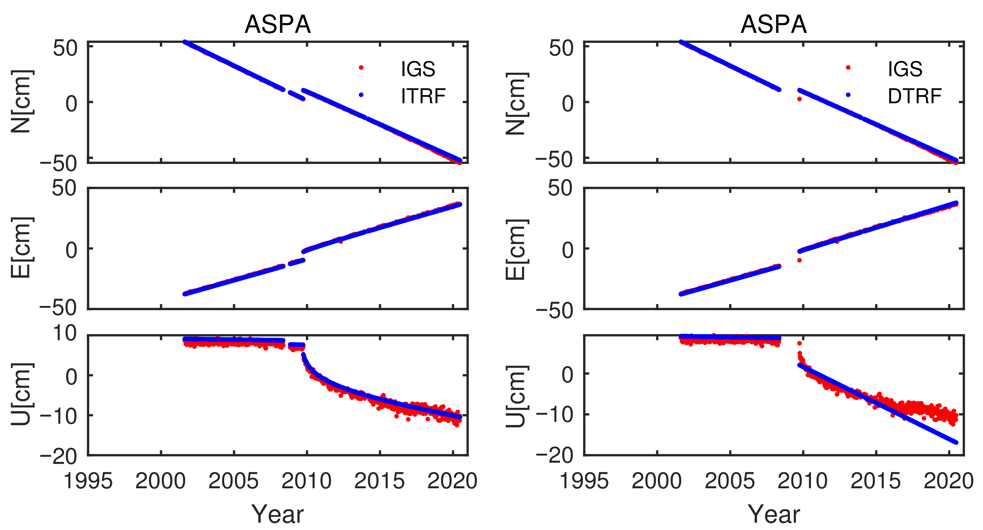
For instance, the coordinate time series of station ASPA are displayed in
Figure 6, where we find that using the ITRF2014 models to fit the IGS time series performed better than the DTRF2014—especially after 31 December 2014. As a post-seismic response may last several years, the affected stations will contain irregular error signals, which is different from systematic errors. Applying NTL models to correct individual daily or weekly solution motions will generate position and velocity differences. Constant offsets exist in most station position time series between DTRF2014 and IGS; however, the magnitude may differ from the previous section in the comparison between ITRF2014 and IGS.
We performed a Helmert transformation between the DTRF2014 and the corrected IGS time series and employed identical outlier rejection condition as utilized in the previous section. The corrected transformation parameter time series and their amplitude spectrums are displayed in
Figure 7. Following the comparison strategy from the previous section, the Helmert parameters were split into two sections at the reference epoch of 2015.0. The drifts and standard deviations that resulted from linear regressions to the transformation parameter time series of the two sections are provided in
Table 2.
The time series of transformation parameters between the DTRF2014 and IGS solutions exhibited distinct linear signals during the determination and prediction periods in all the three components. The drifts of the translations changed from 0.07, 0.11, and −0.15 mm/yr to −0.17, −0.18, and −0.12 mm/yr; the drifts of rotations from −3.6, −1.9, and 2.9 μas/yr to 15.9, −2.3, and 13.2 μas/yr; and the drift of scale offsets from 0.007 to −0.005 ppb/yr. In contrast with the comparison between the ITRF2014 and IGS solutions, the drift of the transformation parameters between DTRF2014 and the IGS solutions showed greater differences between the two sections (particularly for the X component translation and rotation time series). Although complex signals were similarly contained in the time series of the Y and Z component translation parameters, the trends of the two can reveal accuracy degradation of DTRF2014 to an extent.
A mean offset of 0.123 ± 0.135 ppb and a statistical drift of 0.007 ppb/yr were found in the scale offsets before February 2017 as the consequence of the scale processing strategies adopted in averaging the VLBI/SLR information and the constraints at the colocation sites used for the local ties between the two space techniques [
30,
34]. The annual and semiannual amplitudes of the scale offsets were 0.25 ppb and 0.05 ppb, respectively, which are similar to the values estimated between the ITRF2014 and IGS time series.
Except for the non-linear signals in scale offsets, the largest spectral peak less than 0.25 mm was visible in the X component of the translation time series, and other peaks were observed at several harmonics of the GPS draconitic year. For instance, the Z component translation parameters showed distinct peaks at the 6th and 7th harmonics, and the X component rotation parameters showed clear peaks at the 3rd harmonics. All the amplitudes of spectral peaks were slightly unequal to the amplitude spectra estimated between ITRF2014 and IGS, which indicates coordinate differences induced by the different combination strategies, non-linear signal handling, etc.
5. Comparison between JTRF2014 and IGS
Unlike the secular frames ITRF2014 and DTRF2014, the JTRF2014 is a time series-based reference frame realized by combining space geodetic inputs, including VLBI, SLR, GNSS, and DORIS, at a weekly resolution, whose origin is at the quasi-instantaneous CM as measured by SLR. The scale is the weighted average of the quasi-instantaneous scales determined by SLR and VLBI observations. The frame orientation is conventionally aligned to ITRF2008 through the NNR constraint applied to each weekly solution. As a quasi-instantaneous frame, the JTRF2014 attempts to provide station positions by referring to the quasi-instantaneous geocenter position.
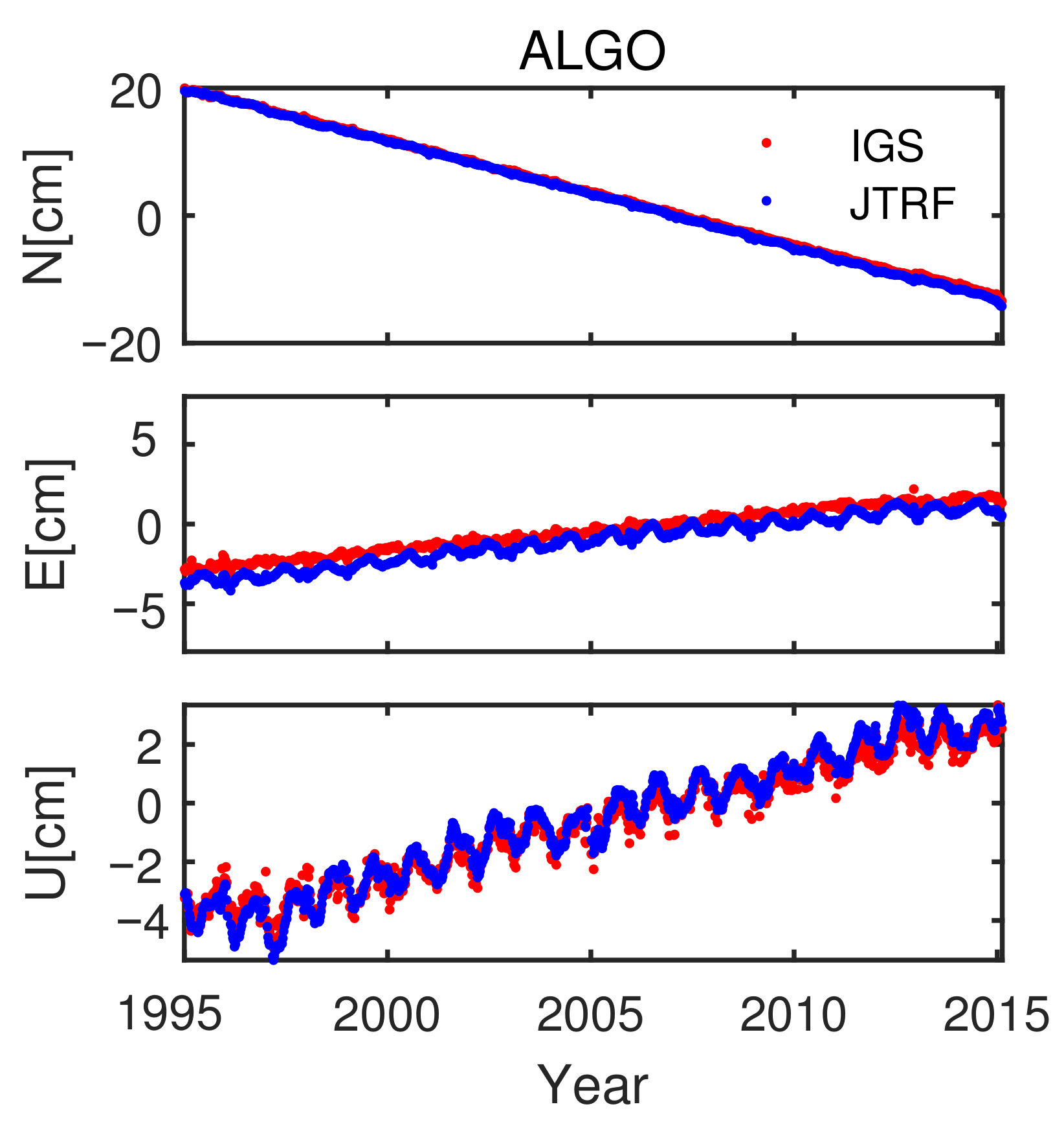
Figure 8 shows the station position time series of ALGO of the IGS and JTRF2014 frames, which indicates not only a constant offset but also unequal amplitudes of the periodic signals between the two position time series. Stable offsets between the two station coordinate time series indicate a long-term mean bias of origin between them. The amplitudes of the periodic signals in JTRF2014 were unequal to IGS because JTRF2014 was constructed as an epoch-like frame, and the subsecular variations of the non-linear geocenter motions and the surface seasonal variations of solid earth are represented in the time series of the realized quasi-instantaneous JTRF2014 frame, while, for the linear frame IGS time series, only surface seasonal variations are included.
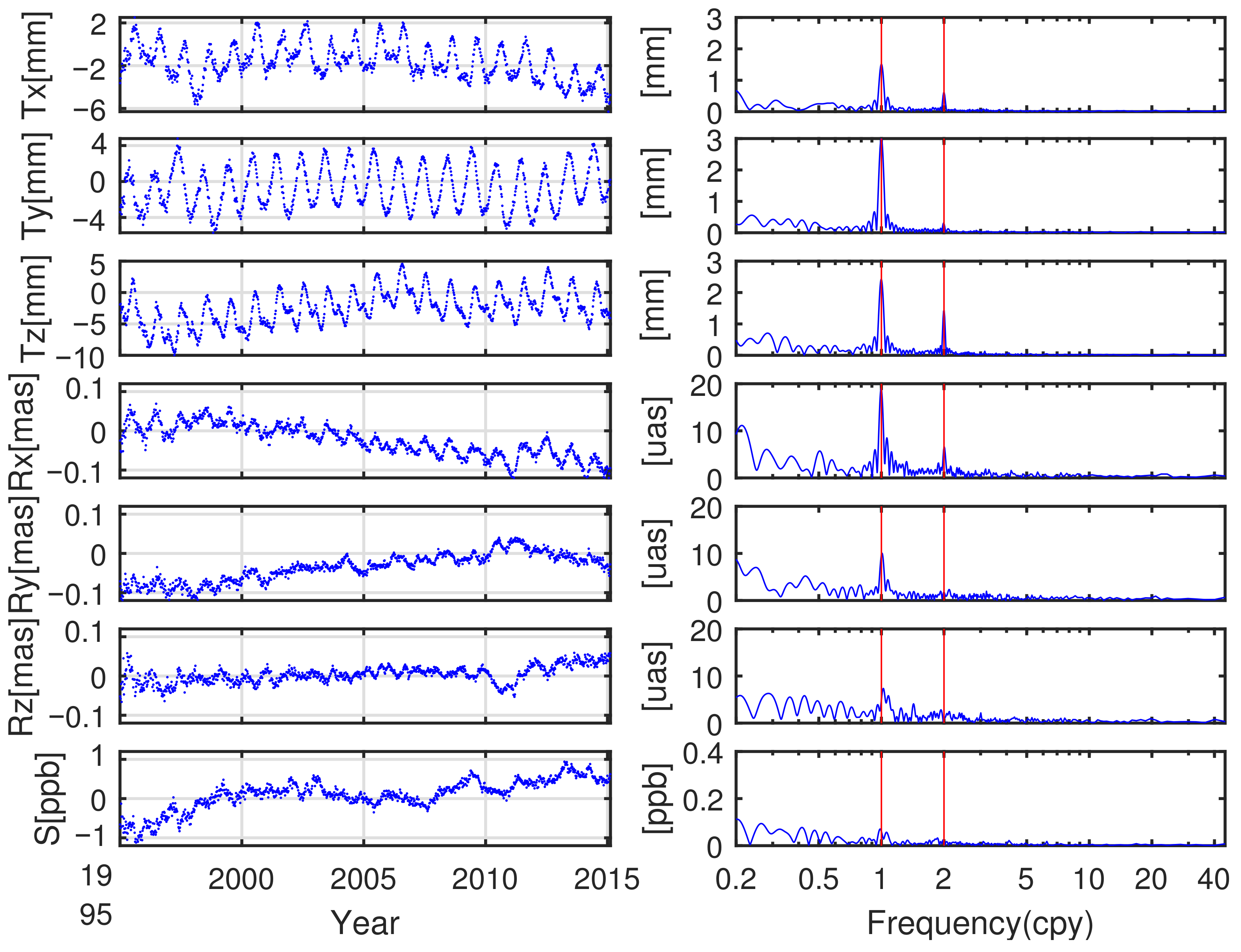
Likewise, a Helmert transformation was performed between JTRF2014 and the corrected IGS solutions. JTRF2014 is a quasi-instantaneous frame and unable to access to the period after February 2015; therefore, only IGS solutions from 1995 to February 2015 are compared in this section. The transformation parameter time series and their amplitude spectra are displayed in
Figure 9. The offset, drift, and standard deviation (STD) that resulted from linear regressions to the transformation parameter time series are provided in
Table 3. The annual and semiannual amplitudes of the translation and rotation parameter time series estimated between JTRF2014 and IGS are provided in
Table 4.
Significant spectrum peaks at the annual and, to a lesser degree, semi-annual frequency, are visible in the amplitude spectra of the translation time series, which reflects the geophysical, and mostly related to mass, transformation of the earth surface, and to a large extent, eventually reflect the seasonal geocentric motion [
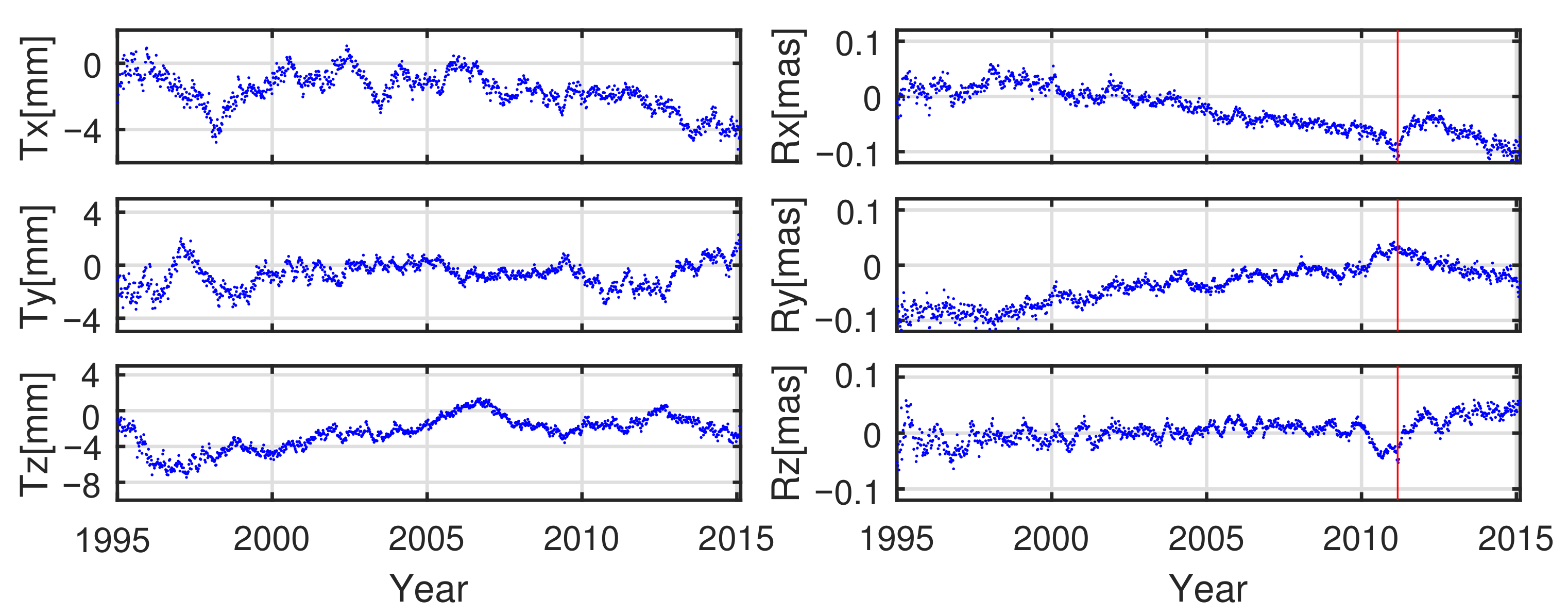
35]. The time series of the translation parameters estimated between JTRF2014 and IGS after subtracting the annual and semiannual signals are displayed in the left panel of
Figure 10, where we see that the Helmert parameters vary with time and could be split into different sessions with the trend of each session diverging from the long-term overall trend.
Linear fits of the translation drifts were statistically zero for the Y components. Drifts of −0.10 and 0.33 mm/yr were found for the X and Z components in the long-term fitting, respectively. The results indicate that the SLR-determined origin was not only nonlinear but also had a short-term variation trend. Therefore, using a long-term averaged origin of SLR observations to describe geocenter motions of the solid earth, as implemented in the determination of the ITRF2014 and DTRF2014 appears not rigorous and would introduce inappropriate errors in geophysical-related research.
The rotation offsets between JTRF2014 and the corrected IGS solutions, together with corresponding amplitude spectra are reported in the fourth to sixth rows of
Figure 9. The annual amplitudes estimated for the X and Y component were 18.6 and 9.7 μas, respectively. In addition, there was an apparent change in the trend of the rotation parameters time series around the epoch 2011.0. Thus, the NNR constraints designed by Wu et al. [
15] may not precisely satisfy the orientation definition of the JTRF2014. In general, the worse consistency between the IGS and JTRF and apparent linear trend that occurred in the three components of −5.72, 4.25, and 2.87 μas/yr was unexpected. How to reduce the seasonal variations and linear discrepancies is a great concern in the next generation ITRF.
Weak seasonal signals and draconitic frequencies of the scale offset time series are shown in
Figure 9. Here, non-linear variation of the selected GNSS network vertical component disappears due to the fact that periodic signals are characterized in both of the two epoch-like frames. The scale discrepancy between JTRF2014 and the corrected IG2 was less than 1 ppb over time (about 7 mm at the equator). In addition, a positive long-term linear varying trend (about 0.05 ppb/yr) can be noticed in the scale offset time series.
Thus, most of the non-linear variations should come from the SLR results. The number of SLR stations shows unstable variations from week to week (see, e.g., Figure 2.16 in Sosnica, 2014 [
36] and Figure 5 in Zajdel et al. 2019 [
37]), from which the geometry variations may be the major factor for the temporal instability in the time series of scale offsets [
38]. The poor geometry of VLBI and co-location sites and the constraints and weightings performed at local ties were also non-negligible factors for the time-dependent trend of the scale differences.
6. Conclusions
The three most recent ITRS realizations, ITRF2014, DTRF2014, and JTRF2014, are regarded as the most accurately realized TRFs thus far. In this paper, the continuous IGS position time series from 1995 to 2020 were used as a reference to investigate the characteristics of the three frames by applying the Helmert transformation approach. The major results from this work are listed as follows:
(1) Datum maintenance of the IGS solutions relied on a minimum constraint applied on a subset of the core stations. Due to the decrease in the core station number used as the datum to align the IGS solutions with the specific IGS frame, the origin differences between the IGS solutions after frame alignment and ITRF2014 reached 1.8 and 2.0 mm in the Y and Z components, respectively.
(2) Due to mismodeling and inappropriate modeling of ITRFs, the orientation of ITRF2014 diverged from the definition orientation (i.e., the orientation of ITRF2008) with drifts of 11.9, 5.5, and 8.4 μas/yr, and the scale of ITRF2014 diverged from the definition with a drift of −0.038 ppb/yr.
(3) Comparing DTRF2014 to the IGS solutions, the origin rate parameters in the X/Y directions and orientation rate parameters in the X/Z directions show distinguished divergences for the determination and prediction periods, where X/Y origin rate parameters change from 0.07, 0.11 mm/yr to −0.17, −0.18 mm/yr and X/Z orientation rate parameters change from −3.6, 2.9 μas/yr to 15.9, 13.2 μas/yr.
(4) For the JTRF2014, its annual signals regarding the origin differences could be up to 1.5, 3.0, and 2.4 mm in the X, Y, and Z components, respectively, and the temporal variation trends were not in accordance with the long-term trend. In addition, except for the larger linear discrepancies and seasonal signals that exist in the X and Y components, a distinct trend switch occurred in the orientation parameters. The temporal variation characteristics of the scale offsets may be related to the weekly ground network variations of SLR, along with the local ties and weights used to combine the SLR and VLBI.


