Abstract
Machine learning and deep learning methods have been employed in the hyperspectral image (HSI) classification field. Of deep learning methods, convolution neural network (CNN) has been widely used and achieved promising results. However, CNN has its limitations in modeling sample relations. Graph convolution network (GCN) has been introduced to HSI classification due to its demonstrated ability in processing sample relations. Introducing GCN into HSI classification, the key issue is how to transform HSI, a typical euclidean data, into non-euclidean data. To address this problem, we propose a supervised framework called the Global Random Graph Convolution Network (GR-GCN). A novel method of constructing the graph is adopted for the network, where the graph is built by randomly sampling from the labeled data of each class. Using this technique, the size of the constructed graph is small, which can save computing resources, and we can obtain an enormous quantity of graphs, which also solves the problem of insufficient samples. Besides, the random combination of samples can make the generated graph more diverse and make the network more robust. We also use a neural network with trainable parameters, instead of artificial rules, to determine the adjacency matrix. An adjacency matrix obtained by a neural network is more flexible and stable, and it can better represent the relationship between nodes in a graph. We perform experiments on three benchmark datasets, and the results demonstrate that the GR-GCN performance is competitive with that of current state-of-the-art methods.
1. Introduction
Hyperspectral image (HSI) classification has received attention due to its applications in environmental monitoring, agriculture, and the military [1,2]. In recent years, many methods have been applied in HSI classification, e.g., k-nearest neighbor (k-NN) [3], support vector machine (SVM) [4], random forest [5], extended morphological profile (EMP) [6], and extreme learning machine [7]. With the success of deep learning in the computer vision [8,9,10,11] and natural language processing [12,13,14] fields, many scholars have attempted to utilize advanced network structures in HSI classification. Chen et al. first introduced the concept of deep learning into HSI classification by using stacked autoencoders [15]. A feature extraction framework based on the deep belief network was proposed by Chen et al. to deeply extract features [16]. Because recurrent neural networks are designed for sequential data, Mou et al. applied them in HSI data analysis [17]. Zhu et al. presented two generative adversarial network (GAN) frameworks, spectral-based and spatial-spectral-based frameworks, and confirmed the usefulness of GAN in HSI classification [18].
Of the deep learning methods used for HSI classification, one widely applied framework is the convolutional neural network (CNN). Hu et al. introduced CNN to HSI classification for the first time as a one-dimensional CNN (1D-CNN) that only used spectral information and exhibited limited accuracy [19]. Various CNN types have been subsequently developed. Makantasis et al. adopted a two-dimensional CNN (2D-CNN), where spectral bands are regarded as feature maps [20]. Chen et al. then systematically compared the 1D-CNN, 2D-CNN, and three-dimensional CNN (3D-CNN), and they provided guidance on CNN structure design [21]. He et al. proposed a multi-scale three-dimensional deep CNN, in which convolution kernels of different sizes were employed in spectral dimension [22]. In addition, Li et al. put forward a novel pixel-pair method to augment the available training samples, with the final classification determined by voting [23]. According to [24], a siamese network composed of two CNNs can be trained to lower intraclass variability and raise interclass variability. In [25], the spectral dimension is cut into several sections, and these sections are parallelly fed into the network to effectively extract features using fewer training parameters, known as BASS net. Additionally, a spatial-spectral residual network (SSRN), where two residual blocks, namely spectral and spatial residual blocks, constitute the end-to-end network, was created. By using residual blocks, SSRN can achieve higher classification accuracy with more layers [26]. To take advantage of the high accuracy of 3D-CNN while reducing the number of training parameters, Roy et al. devised a hybrid network named HybridSN that uses a 3D-CNN to extract low-level features and a 2D-CNN to extract high-level features [27]. Zhang et al. utilized the depthwise and pointwise convolution layers to construct a three-dimensional lightweight CNN, and they adopted transfer learning to alleviate the small sample problem [28]. Additionally, in [29], a 1D-CNN was used to extract spectral features, a 2D-CNN was used to extract spatial-spectral features, and the features were then fused according to a predictive feature weighting mechanism, achieving sufficient classification performance.
As a kind of graph neural network, graph convolution network (GCN), a method to process non-euclidean data, is widely used in the fields of social networks, knowledge graphs, and so on. The following is a brief introduction to the development of GCN and the graph neural network. Bruna et al. extended the convolution operation from Euclidean data to graph-structured data using the spectral domain perspective [30]. Afterwards, quickly localized convolutional filters were designed for graphs by Defferrard et al. using Chebyshev polynomials to approximate the convolution kernels [31]. Kipf et al. further simplified this work by only using the first-order approximation of spectral graph convolutions, and the final result was the basic form of the GCN, which is now widely used [32]. Apart from applying convolution operations in the spectral domain, exploration in the spatial domain has also been made. Considering that the previous work is transductive, meaning that all node details in a graph are required for training, Hamilton et al. proposed an inductive framework named GraphSAGE based on the spatial domain in which a function learns to generate node embeddings [33]. In addition, in [34], Simonovsky et al. formulated edge-conditioned convolution (ECC), where the filter weights depend on the edge labels and vary according to the input samples. Velickovic et al. introduced an attention mechanism to graph neural networks and proposed the graph attention network (GAT) [35]. GraphSAGE, ECC, and GAT are similar, spatial-based approaches.
To the best of our knowledge, graph neural networks were introduced to the HSI classification field within the last three years. Qin et al. proposed a spectral–spatial GCN in which the relation between nodes not only depends on spectral similarity but also spatial distribution [36]. Shahraki et al. applied 1D-CNN to an HSI data to obtain node features, and then they used a semi-supervised adjacency matrix with the previously obtained nodes to perform graph convolution [37]. In [38], the ECC method was deployed for HSI classification, and during the graph construction process, both spectral and spatial information were considered. Hong et al. adopted a mini-batch strategy to train the GCN called miniGCN and investigated the situations of jointly using GCNs and CNNs to extract feature representations [39]. A multi-scale dynamic GCN (MDGCN) was presented by Wan et al. in which the superpixel technique was used to reduce the training complexity, and a multi-scale technique was applied to effectively utilize spatial information [40]. Wan et al. also developed the context-aware dynamic GCN. They proposed a dynamic graph refinement mechanism to obtain a more accurate adjacency matrix and graph projections based on superpixels [41]. Liu et al. extracted EMP features and organized them as graph-structured data to apply a GCN [42]. In addition, Mou et al. employed a nonlocal GCN in which the entire HSI image is fed to the network, requiring high network computational complexity [43]. Apart from applying a GCN in HSI classification through semi-supervised learning, unsupervised learning has also been attempted. For example, Cai et al. presented a new subspace clustering framework based on graph convolution and obtained satisfactory results [44]. GAT has also been innovated for HSI classification as a graph neural network [45,46].
As introduced above, machine learning and deep learning methods are widely used in the field of HSI classification. Among the deep learning methods, the CNN-based methods are the most widely used and become the mainstream technical route. In recent years, GCN, as a kind of graph neural network, has achieved great success in processing graph structure data. Because of its advantages in dealing with the node relationship, researchers introduced GCN to the field of HSI classification. However, there are two crucial problems using GCN in HSI classification. The one is how to transform HSI into the graph structure data which GCN can handle. The other one is how to model the node relationship in the graph structure data we build.
Faced with these, we propose a novel network called Global Random Graph Convolution Network (GR-GCN). Our work was inspired by [47], in which a GCN is applied in the few-shot learning field. The primary contributions of this article are as follows.
- A novel method of constructing the graph in HSI classification is proposed. The method, which we call global random graph-based strategy, can save computing resource, overcome the problem of insufficient samples. Moreover, the diversity of the constructed graphs can make the network more robust.
- A neural network-based method of obtaining an adjacency matrix is proposed. Compared with artificial rules, this method can more effectively mine the internal connections between graph nodes.
- We propose a general end-to-end supervised learning framework based on the GCN for HSI classification. Three benchmark datasets are used to test the proposed framework performance.
2. Proposed Method
2.1. Preliminary Knowledge
Given the graph , with V and E denoting the sets of nodes and edges, define as the adjacency matrix of G, where represents the connection status between the ith and the jth nodes, and as the degree matrix, where the diagonal element . Then, the symmetric normalized Laplacian matrix, the key spectral filtering operator on the graph, is calculated as follows:
where I is the identity matrix, U represents the matrix of the eigenvectors of L, and denotes the diagonal matrix of the eigenvalues of L.
Based on this information, the convolution operation of the graph in the spectral domain can be expressed as follows:
where is a diagonal matrix, elements of which are the parameters to be learned. represents one scalar for each node in the graph. Because Equation (2) requires calculating the eigenvectors of L, it is computationally costly. To overcome this problem, Defferrard et al. [31] used Chebyshev polynomials up to the Kth order to approximate .
where is the Chebyshev polynomial of order K; denotes the polynomial coefficient, which represents the parameters to be trained; and is defined as , where is the largest eigenvalue of L. The purpose of computing is to rescale the to fit the input range of the Chebyshev polynomial. Hence, Equation (2) can be rewritten as
where . The eigendecomposition is circumvented in Equation (4), which is the desired outcome. The suitable nature of the Chebyshev polynomial is also noteworthy. , where , and , meaning that can be obtained recursively.
To further simplify the computational process, Kipf and Welling [32] only utilized two polynomials (the 0th order and 1st order polynomials), and they approximated . By conducting this limiting and approximating, we obtain the following equation.
where and are both polynomial coefficients. By letting ,
The range of is , which may cause gradient explosion or vanishing. Therefore, Kipf and Welling [32] applied a normalization technique that replaced with , where and . As a result, the final GCN model formulation is
where denotes the input graph data of the lth layer, represents the trainable parameter matrix of the lth layer, and is the activate function used in network.
2.2. Construction of Global Random Graph
HSIs typically exhibit a shape of , where H and W are the height and width of the HSI, respectively, and B is the number of spectral bands. First, a principal component analysis is applied to the HSI to remove redundant details in the spectral dimension. Then, the HSI shape becomes , where is the number of reserved principal components. To fully utilize the spatial context, the input into the GR-GCN is the target pixel combined with its neighborhood (called cube in this article), whose shape is , where w is an odd number greater than 1 that refers to the window size limiting the neighborhood scope. To feed pixels near the HSI edge into the network, we fill in a moat around the image with zeros; the width of moat is set to . In the experiment, we take as 30 and w as 25.
We define C as the number of classes in the HSI, n as the number of labeled samples of each class, and as the number of total unlabeled samples. Then we can get the total label set L, the label set with label i , and the unlabeled set U as follows:
where x represents a cube whose shpae is , the superscript i of x means the cube label is i and the superscript u of x means the cube label is unknown.
The graph construction process is described in Figure 1. As illustrated in Figure 1, the train and test graphs are derived from the label and unlabeled sets. The following is the construction process of the train graph. First, k samples are picked randomly from each label set so that we can obtain samples called supported nodes. After that, we select one sample from remaining samples in total label set and call it target node. The support nodes and the target node together constitute the train graph. The test graph composition is nearly the same as that of the train graph. The only difference is that the target node in test graph is from the unlabeled set and not from the total label set. We can observe that there are nodes in both the train graph and test graph.
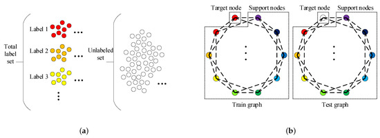
Figure 1.
(a) is the schematic diagram of the label sets and unlabeled set. (b) is the schematic diagram of the train graph and test graph. Both the train graph and test graph are derived from the label sets and unlabeled set and composed of one target node and support nodes. The support nodes in both train graph and test graph are obtained by randomly selecting k samples from each label set, and there are total C label sets. The schematic diagram actually depicts the situation when . The one target node in train graph is obtained by randomly selecting one sample from total label set. The one target node in test graph is obtained by randomly selecting one sample from unlabeled set.
Then we discuss the number of available graphs below. From the description of the graph construction process, it can be known that the number of available train graphs and the number of available test graphs are respectively:
Let us take the University of Pavia dataset (one of the datasets we used in the experiments) as an example. In this dataset and we assume that n and k are 200 and 1 respectively, then can be determined and is equal to 40,976. According to Equations (11) and (12), the magnitude of train graph number we obtain is and the magnitude of test graph number is . It is apparent that by using this strategy, the available train graphs is sufficient. However, it is neither possible nor necessary to traverse all the train graphs due to their large number. In the experiment, we used the mini-batch learning method for training, and set the batch size to 200, the batch number to 500. Therefore, the total number of train graphs we used is 100,000. In subsequent section, we will discuss the loss convergence and accuracy of our proposed GR-GCN as the batches fed into network increases. The number of available test graphs is huge as well. But for one target node to classify, we only use one corresponding test graph. In other words, when trianing is accomplished, our proposed network is capable of distinguishing the given target node only using a set of support nodes picked randomly. In subsequent section, we will discuss the dependence of target node classification accuracy on support node selection. In the experiments, We set n and k as 200 and 2 respectively. The hyperparameter n associates with the number of available label samples, and the hyperparameter k associates with the number of nodes in graphs we construct. The impact of these two key hyperparameters will be discussed in a subsequent section.
Introducing the GCN, a method of processing non-euclidean data, into the field of HSI classification, a key issue is how to transform HSI, a typical euclidean data, into non-euclidean data. Different researchers have given different solutions. In [36,37,38,39,42], the researchers searched for samples to construct neighbor nodes based on the similarity of spectra, supplemented by spatial constraints (called spectrum-based method in this article). In [40,41], the researchers first merged pixels into superpixels with the superpixel technique and then determined the neighbor nodes based on the connection in space (called superpixel-based method in this article). And in [43], the researchers considered all the other samples when considering the neighbor nodes of a sample, which relies on the powerful computing capacity (called entirety-based method in this article). We propose a novel method of constructing the graph in HSI classification called the global random graph method. There are three main advantages of using the global random graph-based method as follows:
(1) The size of each global random graph is small. The above three methods all use the whole samples to form graph nodes. For both the spectrum-based method and the entirety-based method, the number of nodes in the constructed graph is tens of thousands. Even for the superpixel-method which applies the superpixel technique, there are still thousands of nodes in the constructed graph. However, for our proposed method, the size of each global random graph is quite small. Let us continue taking the University of Pavia dataset as an example and there are only 10 nodes in the global random graph with k assumed to 1. Therefore, the computing resources occupied by the scale of the global random graph are very limited. Actually, the most computational resource occupancy of the proposed network is in the parallel feature extraction network.
(2) The number of available global random graphs is huge. As described above, the global random graph-based method significantly increases the available train graphs. We can declare that using the global random graph-based method largely overcomes the problem of insufficient label samples.
(3) Randomness is introduced through permutation and combination. We tend to regard the global random graph as a lookup table by which we can identify the target node relying on the associations between the target node and support nodes. This is why the diversity of node combinations is needed, because only in this way can the trained network be more robust and adapt to various situations. The randomness introduced by permutation and combination satisfies this diversity. For the spectrum-based method, similar samples in the spectral dimension are considered as neighbor nodes in the graph. For the superpixel-based method, it is based on the connection in space. These two methods both consider only a limited number of samples as neighbor nodes. Although the entirety-based method considers the relationship between any two samples, it requires large computing resources. Using simple permutation and combination, the global random graph-based method not only satisfies the diversity but also does not require excessive computing resources.
2.3. The Overview of GR-GCN
The framework of GR-GCN is displayed in Figure 2. In the schematic diagram, the gray arrows indicate the flow of data.
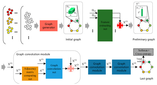
Figure 2.
The framework of Global Random Graph Convolution Network (GR-GCN). The gray arrows indicate the flow of data. First, using the graph generator with a random mechanism, we obtain the initial graph. Then, the initial graph nodes are fed into feature extracting net parallelly to extract features and we combine the extracted features forming a graph called the preliminary graph. After that, the preliminary graph passes through three graph convolution modules and transforms into the last graph. Finally, we apply the softmax/cross-entropy loss function to the target node of the last graph. There are two symbols worthy to note. The red symbol “+” refers to splicing N tensors, whose shapes are all , into one tensor whose shape is . The pink symbol “+” refers to splicing two tensors, whose shapes are and , into one tensor whose shape is . Here, a, b, and N are only for illustration.
First, using the graph generator with a random mechanism, we can obtain a graph called the initial graph. The initial graph node is the cube denoted by (the subscript j denotes the jth node in the graph) whose shape is . It is worth noting that the initial graph is just in an embryonic form because the node features and the relationship between nodes are not determined yet.
Then, we feed the initial graph nodes into the feature extracting net parallelly and obtain a graph called the preliminary graph. The preliminary graph node is the feature vector that is extracted by the feature extracting net and denoted by (the subscript j denotes the jth node in the graph) whose shape is . refers to the set of node features in the preliminary graph. Although the node features of the preliminary graph are obtained, the preliminary graph is still not complete due to the absence of the adjacency matrix.
After that, data passes through three graph convolution modules and transforms into a graph called the last graph, which is the graph we use to classify. The graph convolution module is composed of the adjacency matrix computing net and the graph convolution net. For conciseness, Figure 2 only shows the composition of one of three graph convolution modules. In the graph convolution module, the adjacency matrix computing net is responsible for obtaining the adjacency matrix. Therefore, the graph becomes complete after using the adjacency matrix computing net and is fed to the subsequent graph convolution net. In Figure 2, refers to the set of node features and denotes the adjacency matrix in the corresponding graph. The superscript i in and indicates the location in the network.
Finally, the softmax/cross-entropy loss function is applied to the target node of the last graph to train the proposed network.
To obtain additional insight into the GR-GCN, the shape details of data flow are listed in Table 1, in which is the feature number of , and J is the channel number of the adjacency matrix. It is worth mentioning that and are not shown in Figure 2 and they are adjacency matrices obtained in the second and third graph convolution module respectively.

Table 1.
The shape of essential datas in GR-GCN.
2.4. The Feature Extracting Net
Figure 3 shows the main architecture of the feature extracting net and Table 2 displays the details of each layer in the feature extracting net. It can be seen that the feature extracting net is essentially a 3D-CNN, used for extracting features from the target pixel and its neighborhood. Using the 3D-CNN, the feature extracting net utilizes not only spectral information but also spatial information. Furthermore, the extracted high-level and abstract features are more conducive to the subsequent classification task. In follow-up experiments, the ablation experiment will be conducted to illustrate the role of the feature extracting net and its impact on classification accuracy.
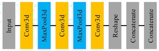
Figure 3.
The architecture of feature extracting net.
Table 2.
The details of each layer in the feature extracting net.
There are two details that need to be elaborated. The one is that in the first concatenate layer, we need to code the sample label into the one-hot format and concatenate it to the extracted features. After that, N individual sample features are concatenated forming the set of node features , from which we can see that . The other is that there is no activate layer in the feature extracting net because adding the activation layer after the convolutional layer reduces the classification accuracy by to . The reason for this phenomenon may be that introducing excessive nonlinearity to the network results in inaccurate network convergence.
2.5. The Graph Convolution Module
As Figure 2 shows, there are three graph convolution modules. As described above, the graph convolution module consists of the adjacency matrix computing net and the graph convolution net. In the graph convolution module, the set of node features first is fed to the adjacency matrix computing net to obtain the adjacency matrix. Then, the set of node features, with the adjacency matrix, passes through the graph convolution net to further extract features. Finally, the features extracted by the graph convolution net are combined with the previous features as the input of the subsequent module. This operation draws trick from the residual network [10] and aims to make the features more representative and prevent network degradation.
Figure 4 shows the main architecture of the adjacency matrix computing net and Table 3 displays the details of each layer in the adjacency matrix computing net. Before feeding into the adjacency matrix computing net, a metric should be applied to to quantify the bonds between each node in the graph. The metric is calculated as
where either or is the features of any node in (the subscript p and q denote the pth and qth node in the graph. The subtraction and absolute value operators both occur at the element level. Despite the simplicity of the metric, it is demonstrated to be effective in the experiment. It can be seen that the adjacency matrix computing net is essentially a 2D-CNN. In the adjacency matrix computing net, we stack multiple 2D convolution layers with convolution kernels and take the final feature map as the adjacency matrix. This approach seems slightly rough, but the end-to-end training method makes it work well. In pioneer works that employ GCN in HSI classification, the adjacency matrix is typically calculated using a distance metric, and then the adjacency matrix is fixed. Compared with the artificial rules, a neural network based on trainable parameters is more flexible and can more precisely investigate the associations between nodes in a graph. At the end of the network, considering the relationship between the node and itself in the graph, an identity matrix is concatenated to the adjacency matrix, which means that .
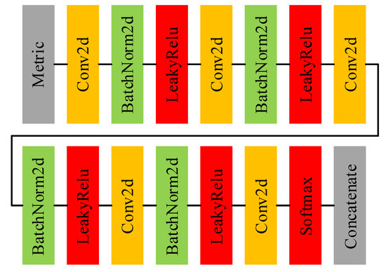
Figure 4.
The architecture of adjacency matrix computing net.
Table 3.
The details of each layer in the ith adjacency matrix computing net.
Table 4 displays the details of the graph convolution net. The graph convolution net is the application of Equation (7), in which the W denotes the parameters that need to be trained in the graph convolution net. The first and second graph convolution net output feature numbers are both 48, whereas that of the third graph convolution net is C. From Table 1 and Figure 2, we can obtain the relationships between the , , , and , which are , , and , respectively.
Table 4.
The feature number of input and output of ith GCN.
2.6. Some Hyperparameters
The softmax/cross-entropy loss function is applied to the target node, which is split from the last graph, and the Adam optimizer is selected to train the GR-GCN. The parameters in the network are randomly initialized, and the learning rate is set to to update these parameters. We use the mini-batch learning method and set the batch size to 200, the batch number to 500.
3. Datasets and Experimental Setup
3.1. Datasets
Three widely used HSI datasets are employed in our experiments, including the Indian Pines, Salinas, and University of Pavia datasets.
- The Indian Pines dataset was obtained using the Airborne Visible Infrared Imaging Spectrometer (AVIRIS), which is in size and contains 220 spectral channels. After removing 20 water absorption bands, we obtain corrected data with 200 spectral bands. And the spatial resolution is 20 m per pixel. There are a total of 16 land-cover classes; only 12 of them are used in the experiments due to an insufficient number of samples in certain categories.
- The University of Pavia dataset was collected using the Reflective Optics System Imaging Spectrometer, which is in size and contains 103 spectral channels. And the spatial resolution is m per pixel. There are 9 land-cover classes in the dataset, and all of them are used in the experiments.
- The Salinas dataset was also gathered using the AVIRIS, which is in size and contains 224 spectral channels. Similar to the Indian Pines dataset, a correcting operator is applied to the Salinas dataset, and 204 spectral bands remain afterward. And the spatial resolution is m per pixel. There are 16 land-cover classes in the dataset, and all of them are used in the experiments.
The number of training and testing samples for each category of the three datasets is listed in Table 5, Table 6 and Table 7. The dataset pseudo color images fused by certain bands and ground truth images are displayed in Figure 5, Figure 6 and Figure 7. The classes that are not used in the experiments are not in the ground truth images.
Table 5.
The number of label and unlabeled samples for each category in Indian Pines dataset.
Table 6.
The number of label and unlabeled samples for each category in University of Pavia dataset.
Table 7.
The number of label and unlabeled samples for each category in Salinas dataset.
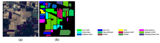
Figure 5.
Indian Pines dataset’s pseudo color image fused of some bands (bands 9, 19 and 29) and ground truth image. (a) pseudo color image; (b) ground truth image.
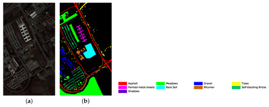
Figure 6.
University of Pavia dataset’s pseudo color image fused of some bands (bands 9, 19 and 29) and ground truth image. (a) pseudo color image; (b) ground truth image.
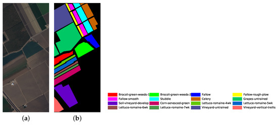
Figure 7.
Salinas dataset’s pseudo color image fused of some bands (bands 9, 19 and 29) and ground truth image. (a) pseudo color image; (b) ground truth image.
3.2. Experimental Setup
Certain machine learning-based, CNN-based and GCN-based methods are compared with our proposed method. Of the machine learning-based methods, we use k-NN and SVM as references. Of the CNN-based methods, 1D-CNN [19], 2D-CNN [20], and BASS [25], classic methods based on CNNs, are selected for comparison. Of the GCN-based methods, the original GCN with no modifications [32], miniGCN [39], and MDGCN [40] are chosen for comparison.
For the k-NN method, the parameter k, the number of nearest neighbors, is determined using a grid search, in which k is set as . The SVM method optimal parameters are also determined using a grid search algorithm. Two types of kernel functions are tested, linear and radial basis function (RBF) kernels. The regularization parameter C is searched for in during the linear kernel grid search process. In the RBF kernel process, the regularization parameter C is searched for in , and the kernel coefficient is searched for in .
The 1D-CNN model is trained for 10000 epochs with a batch size of 256, and the other settings are consistent with those of [19]. Because certain details regarding 2D-CNN are not disclosed in [20], we select the parameters ourselves to achieve the same accuracy. An SGD optimizer is used to train 2D-CNN model, and the learning rate is set to . We use mini-batches 32 in size and train the network for 2000 epochs. The data we apply in the BASS model experiment is the corrected data after the water absorption bands are removed, whereas [25] implements the original data. Therefore, the experiment model architecture has a few differences with that in [25]. Specifically, the model in [25] contains 10 parallel networks with a bandwidth of 22 for the Indian Pines dataset and 14 parallel networks with a bandwidth of 16 for the Salinas dataset. However, in our experiments, 10 parallel networks with a bandwidth of 20 are set for both the Indian Pines and Salinas datasets. Training occurrs for 500 epochs, and the other settings are the same as those described in [25].
For the original GCN model, the k-NN algorithm is applied to acquire the most similar pixels in spectral domain, and the key parameter k is set to 20. Then, Equation (14) is employed to calculate adjacency matrix element
where represents the element of the adjacency matrix located in row i and column j; d is the distance computed by the k-NN algorithm; is the coefficient that controls the exponential function shape; and denotes the set of k nearest neighbors obtained using the k-NN method. Using Equation (14), a sparse adjacency matrix is acquired, which is necessary for the GCN. For the GCN structure, we select a two-layer GCN, with the hidden layer in the middle containing 25 units. The learning rate is set to , and the maximum epoch is set to 500 for training. As for miniGCN and MDGCN models, all the settings are consistent with those of [39,40].
3.3. Implementation Platform
The k-NN and SVM methods are both implemented using a scikit-learn library, and the other methods, which are all deep learning-based, are implemented using a PyTorch library. The experiments are conducted on a server equipped with a single NVIDIA Tesla V100 graphics processing unit (GPU) with 16 GB of memory and 12 GB of random access memory.
4. Results and Discussion
The methods based on the CNN (1D-CNN, 2D-CNN, and BASS) are superior to the machine learning methods (k-NN and SVM) for all three datasets, although the SVM test accuracy is close to that of the 1D-CNN and 2D-CNN for certain datasets. The experiment results demonstrate the superiority of CNN-based methods, which is why CNN has been widely used in HSI classification in recent years. We can see that the original GCN results are only slightly superior to those of the k-NN, and they are inferior to those of the SVM. However, as the GCN-based method continues to be explored, the GCN-based methods keep improving and getting competitive results, such as the MDGCN model and our proposed GR-GCN model. This can show the potential and prospects of the GCN-based method in dealing with the HSI classification. Overall, although the GCN-based method is not as intuitive as the CNN-based method when applied to the HSI classification, with continuous exploration, the GCN-based method shows its potential and prospects in dealing with the HSI classification.
The proposed GR-GCN outperforms all the other methods for all evaluation criteria including OA, AA, and Kappa. For the Indian Pines dataset, compared with the SVM, BASS, and MDGCN methods, the GR-GCN increases the OA by , , and , respectively. For the University of Pavia dataset, compared with the SVM, BASS, and MDGCN methods, the GR-GCN increases the OA by , , and , respectively. For the Salinas dataset, compared with the SVM, BASS, and MDGCN methods, the GR-GCN increases the OA by , , and respectively. The GR-GCN is superior both quantitatively and qualitatively compared to the other methods. The visual effect of the classification maps in Figure 8, Figure 9 and Figure 10 agree with the data in Table 8, Table 9 and Table 10. The GR-GCN classification maps exhibit fewer noises, which indicates a lower misclassification rate than that of the other methods, especially for the Indian Pines and Salinas datasets. For the Salinas dataset, the GR-GCN achieves a test accuracy of . Moreover, the two land covers types that are easily misclassified by other methods, grapes-untrained and vineyard-untrained, can be distinguished well by the GR-GCN. Based on these results, we can conclude that the GR-GCN model surpasses traditional machine learning methods and is comparable with state-of-the-art CNN-based methods. In addition, among the GCN-based methods, the GR-GCN performance far exceeds that of the original GCN and miniGCN, and is competitive compared with MDGCN, which verifies the effectiveness of the techniques utilized in the GR-GCN method.
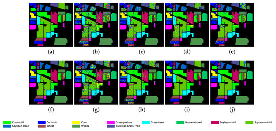
Figure 8.
Classification map for Indian Pines dataset using different methods. (a) Ground truth map; (b) k-NN; (c) SVM; (d) 1D-CNN; (e) 2D-CNN; (f) BASS; (g) GCN; (h) miniGCN; (i) MDGCN; (j) GR-GCN.
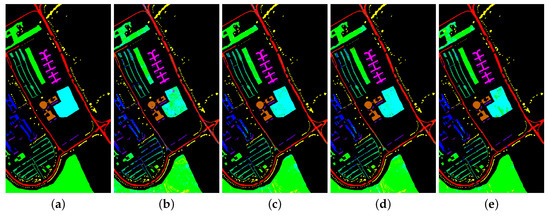
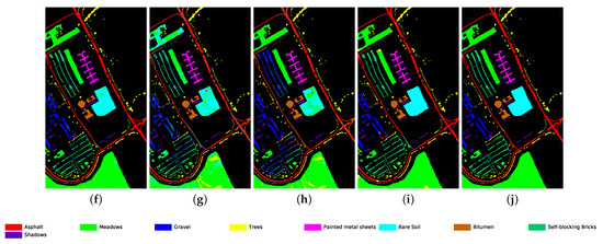
Figure 9.
Classification map for University of Pavia dataset using different methods. (a) Ground truth map; (b) k-NN; (c) SVM; (d) 1D-CNN; (e) 2D-CNN; (f) BASS; (g) GCN; (h) miniGCN; (i) MDGCN; (j) GR-GCN.
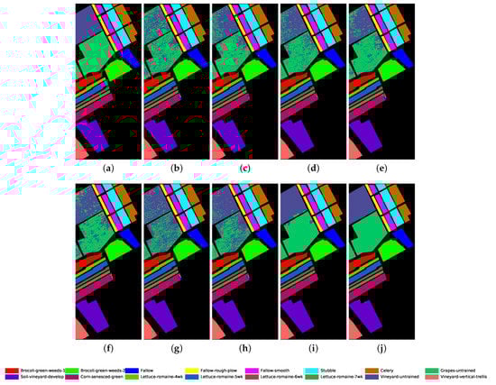
Figure 10.
Classification map for Salinas dataset using different methods. (a) Ground truth map; (b) k-NN; (c) SVM; (d) 1D-CNN; (e) 2D-CNN; (f) BASS; (g) GCN; (h) miniGCN; (i) MDGCN; (j) GR-GCN.
Table 8.
Class specific accuracy, overall accuracy (OA), average accuracy (AA) and kappa coefficient (Kappa) of different methods for Indian Pines dataset.
Table 9.
Class specific accuracy, overall accuracy (OA), average accuracy (AA) and kappa coefficient (Kappa) of different methods for University of Pavia dataset.
Table 10.
Class specific accuracy, overall accuracy (OA), average accuracy (AA) and kappa coefficient (Kappa) of different methods for Salinas dataset.
4.1. The Accuracy and Loss Convergence
For further exploring the model optimization, we display the loss convergence and classification accuracies of our proposed GR-GCN as the batches fed into the network increase in Figure 11. In Figure 11, the orange line corresponds to the train data and the blue line corresponds to the verification data. All hyperparameters are the same as those described above, except that the validation data is added. The verification data is composed of 500 batches, each of which contains 200 random test graphs, and it is worth noting that the verification data does not participate in the backward propagation. As shown in Figure 11, as the batches fed into the network increase, the training and verification accuracy simultaneously improve and the training and verification loss simultaneously converge. The accuracy and loss curves prove that the model we proposed has a good generalization ability, and no over-fitting phenomenon occurs. It can be seen that the convergence is basically completed in the 200th batch, which demonstrates the GR-GCN’s optimization efficiency.
Figure 11.
The loss convergence and classification accuracies of our proposed GR-GCN as the batches fed into network increase. (a) classification accuracies; (b) loss convergence.
4.2. The Ablation Experiment of Feature Extracting Net
To investigate the role of the feature extracting net, the following experiments are conducted. Figure 12 shows the loss convergence and classification accuracies of our proposed GR-GCN with four different configurations. The parameters used in configuration 4 are the parameters of the experiment described above, namely the ultimate version of GR-GCN. Configuration 1 does not adopt feature extracting net but directly inputs the one-dimensional spectral data to the graph convolution module. Configuration 2 uses some regularization techniques, such as batch normalization, on the basis of configuration 1. Configuration 3 adopts feature extracting net but utilizes fewer neighborhoods of the target pixel, setting w as 15.
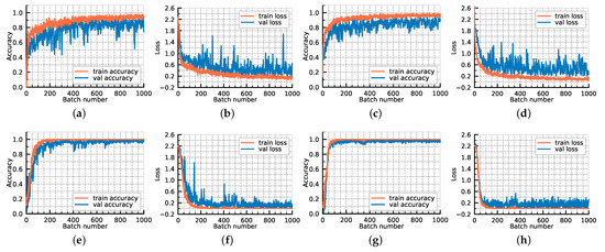
Figure 12.
The loss convergence and classification accuracies of our proposed GR-GCN with four different configurations. (a,b) configuration 1; (c,d) configuration 2; (e,f) configuration 3; (g,h) configuration 4.
The comparison of configuration 1 and 4 illustrates the abstract features extracted from spectral-spatial information are more conducive than only spectral information. The comparison of configuration 2 and 4 demonstrates that the global random graph technique can achieve relatively satisfying accuracy and robustness even without using spatial information. The comparison of configuration 3 and 4 probes the influence of hyperparameter w, and the result shows that a larger value of w can make the model converge faster and fit better.
4.3. The Effect of Support Node Selection
For one target node to classify, we only use one corresponding test graph whose support nodes are randomly selected. Therefore it is necessary to check whether the random selection strategy of the support nodes is effective. The experiment is conducted using the University of Pavia dataset. For each category, we randomly choose 10 unlabeled samples as the target nodes to test. And for each target node, we randomly select 1000 sets of support nodes constructing 1000 test graphs. Table 11 shows the percentage of correct predictions using the 1000 test graphs for each target node. From Table 11, we can see that completely random selection of support node can make correct prediction for target node, which demonstrate the effectiveness and the robustness of our GR-GCN.
Table 11.
Employing GR-GCN to University of Pavia, we randomly choose 10 unlabeled samples as the target nodes for each category. And for each target node, we randomly select 1000 sets of support nodes constructing 1000 test graphs. Here is the the percentage of correct predictions.
4.4. The Impact of Labeled Sample Number n
The number of labeled samples can affect the classification accuracy significantly, there are more labeled samples, the classification accuracy is higher. To investigate the performance of GR-GCN and other competitors under different numbers of labeled samples, we conduct the following experiments. All the methods above are employed under different numbers of labeled samples per class which range from 50 to 200 with a step of 50. And we repeat the experiments in Indian Pines, University of Pavia, and Salinas, and take OA as the metric. The results are shown in Figure 13. As can be seen from Figure 13, except in the experiments in which the labeled sample number is set 50 in Indian Pines and University of Pavia datasets, GR-GCN outperforms the other competitors regardless of the number of labeled samples, no matter in Indian Pines, University of Pavia, or Salinas. The reason why MDGCN performs well when the labeled sample number is small is that it applies a superpixel technique and it is a semi-supervised method that can use unlabeled sample information.
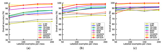
Figure 13.
Overall accuracies of different methods as the number of labeled samples varies. (a) Indian Pines; (b) University of Pavia; (c) Salinas.
4.5. The Influence of Hyperparameter k
According to the graph-constructing process, we can presume that the number of samples picked randomly from each sample set k influences the classification accuracy. We employ GR-GCN for three datasets with different k values, which varied from 1 to 3 at an interval of 1. As illustrated in Table 12, we do not obtain the accuracy for the Salinas dataset when k is 3 because the GPU run out of memory under these conditions. Because as the value of k increases, the cost of computing resources dramatically increases due to the feature extracting net. Based on Table 12, as the k value increases from 1 to 2, the classification accuracy improves, which is in line with our expectations. However, when the k value increases from 2 to 3, the classification accuracy declines slightly, which is probably due to intra-class difference. Therefore, we set k as 2 in the experiments. Setting k as 1 is also a suitable choice because when k is 1, high accuracy is achieved, and the cost of the computing resources is low.
Table 12.
Overall accuracies of GR-GCN under different hyperparameter k, the number of samples picked randomly from each label set, for Indian Pines, University of Pavia, and Salinas.
4.6. Running Time
Running time is an important indicator of deep learning method performance as it affects whether the method can be deployed in real-world applications. Both CNN-based and GCN-based methods are tested using the three datasets, and the results are listed in Table 13, where the training and testing times are reported as the evaluation index. The running time measured for the GCN-based methods includes the graph-building time to make a fairer comparison between the various methods.
Table 13.
The training time and testing time, both in seconds, of various deep learning methods for Indian Pines, University of Pavia, and Salinas.
Based on the results listed in Table 13, we can see that the training time of GR-GCN has its strengths and weaknesses compared with other methods, but it is basically in the same order of magnitude. However, the GR-GCN testing time is substantially longer than the other methods, which is unexpected. The training time can be reduced by using a smaller k value or by terminating the training process in advance. As displayed in Table 13, using a small k value can cut the training time nearly in half. Terminating the training process in advance is effective because the loss convergence is achieved in approximately the 200th batch out of 500 batches. In contrast, testing time can only be reduced by using a smaller k value, which is severely limited. After analyzing the GR-GCN structure, we find that a graph must be constructed for each HSI pixel tested, which makes the testing process costly. Higher cost of testing may be the main limitation of our proposed GR-GCN, and the future work will focus on decreasing the testing time.
5. Conclusions
In this article, we have proposed a novel end-to-end supervised framework named GR-GCN for HSI classification. Two techniques are applied in GR-GCN, constructing the graph for HSI classification in a novel manner and using the neural network to obtain the adjacency matrix necessary for GCN. Using the former technique, the size of the constructed graph is small, which can save computing resources. Besides, we can obtain an enormous quantity of graphs, which can overcome the problem of insufficient samples. Moreover, the random combination of samples can make the generated graph more diverse and make the network more robust. Using the latter technique, we obtain a more reliable and precise adjacency matrix by which high-precise classification can be achieved. Three benchmark datasets have been selected to test the performance of our proposed GR-GCN, and the results indicate that our method is both quantitatively and qualitatively competitive with current state-of-the-art methods.
Author Contributions
C.Z. programmed, analyzed the results and wrote the paper; J.W. was responsible for project administration and the methodology; K.Y. revised the paper. All authors have read and agreed to the published version of the manuscript.
Funding
This research received no external funding.
Conflicts of Interest
The authors declare no conflict of interest.
Abbreviations
The following abbreviations are used in this manuscript:
| HSI | hyperspectral image |
| CNN | convolution neural network |
| GCN | graph convolution network |
| GR-GCN | Global Random Graph Convolution Network |
| k-NN | k-nearest neighbor |
| SVM | support vector machine |
| EMP | extended morphological profile |
| GAN | generative adversarial network |
| 1D-CNN | one-dimensional convolution neural network |
| 2D-CNN | two-dimensional convolution neural network |
| 3D-CNN | three-dimensional convolution neural network |
| BASS | Band-Adaptive Spectral-Spatial Feature Learning Neural Network |
| SSRN | Spatial-Spectral Residual Network |
| HybridSN | Hybrid Spectral Convolutional Neural Network |
| GraphSAGE | Graph SAmple and aggreGatE |
| ECC | edge conditioned graph convolutional network |
| GAT | graph attention network |
| miniGCN | mini-batch graph convolution network |
| MDGCN | Multi-scale Dynamic Graph Convolutional Network |
| AVIRIS | Airborne Visible Infrared Imaging Spectrometer |
| RBF | radial basis function |
| GPU | graphics processing unit |
| OA | overall accuracy |
| AA | average accuracy |
| Kappa | kappa coefficient |
References
- Ghamisi, P.; Plaza, J.; Chen, Y.; Li, J.; Plaza, A.J. Advanced spectral classifiers for hyperspectral images: A review. IEEE Geosci. Remote Sens. Mag. 2017, 5, 8–32. [Google Scholar] [CrossRef]
- Li, S.; Song, W.; Fang, L.; Chen, Y.; Ghamisi, P.; Benediktsson, J.A. Deep learning for hyperspectral image classification: An overview. IEEE Trans. Geosci. Remote Sens. 2019, 57, 6690–6709. [Google Scholar] [CrossRef]
- Blanzieri, E.; Melgani, F. Nearest neighbor classification of remote sensing images with the maximal margin principle. IEEE Trans. Geosci. Remote Sens. 2008, 46, 1804–1811. [Google Scholar] [CrossRef]
- Melgani, F.; Bruzzone, L. Classification of hyperspectral remote sensing images with support vector machines. IEEE Trans. Geosci. Remote Sens. 2004, 42, 1778–1790. [Google Scholar] [CrossRef]
- Gislason, P.O.; Benediktsson, J.A.; Sveinsson, J.R. Random forests for land cover classification. Pattern Recognit. Lett. 2006, 27, 294–300. [Google Scholar] [CrossRef]
- Benediktsson, J.A.; Palmason, J.A.; Sveinsson, J.R. Classification of hyperspectral data from urban areas based on extended morphological profiles. IEEE Trans. Geosci. Remote Sens. 2005, 43, 480–491. [Google Scholar] [CrossRef]
- Pal, M. Extreme-learning-machine-based land cover classification. Int. J. Remote Sens. 2009, 30, 3835–3841. [Google Scholar] [CrossRef]
- Krizhevsky, A.; Sutskever, I.; Hinton, G.E. Imagenet classification with deep convolutional neural networks. In Proceedings of the Advances in Neural Information Processing Systems (NIPS), Lake Tahoe, NV, USA, 3–6 December 2012; pp. 1097–1105. [Google Scholar]
- Ren, S.; He, K.; Girshick, R.; Sun, J. Faster r-cnn: Towards real-time object detection with region proposal networks. In Proceedings of the Advances in Neural Information Processing Systems (NIPS), Montreal, QC, Canada, 7–12 December 2015; pp. 91–99. [Google Scholar]
- He, K.; Zhang, X.; Ren, S.; Sun, J. Deep residual learning for image recognition. In Proceedings of the IEEE Computer Society Conference on Computer Vision and Pattern Recognition (CVPR), Las Vegas, NV, USA, 27–30 June 2016; pp. 770–778. [Google Scholar]
- Redmon, J.; Divvala, S.; Girshick, R.; Farhadi, A. You only look once: Unified, real-time object detection. In Proceedings of the IEEE Computer Society Conference on Computer Vision and Pattern Recognition (CVPR), Las Vegas, NV, USA, 27–30 June 2016; pp. 779–788. [Google Scholar]
- Hochreiter, S.; Schmidhuber, J. Long short-term memory. Neural Comput. 1997, 9, 1735–1780. [Google Scholar] [CrossRef]
- Bahdanau, D.; Cho, K.; Bengio, Y. Neural machine translation by jointly learning to align and translate. arXiv 2014, arXiv:1409.0473. [Google Scholar]
- Devlin, J.; Chang, M.W.; Lee, K.; Toutanova, K. Bert: Pre-training of deep bidirectional transformers for language understanding. arXiv 2018, arXiv:1810.04805. [Google Scholar]
- Chen, Y.; Lin, Z.; Zhao, X.; Wang, G.; Gu, Y. Deep learning-based classification of hyperspectral data. IEEE J. Sel. Top. Appl. Earth Obs. Remote Sens. 2014, 7, 2094–2107. [Google Scholar] [CrossRef]
- Chen, Y.; Zhao, X.; Jia, X. Spectral–spatial classification of hyperspectral data based on deep belief network. IEEE J. Sel. Top. Appl. Earth Obs. Remote Sens. 2015, 8, 2381–2392. [Google Scholar] [CrossRef]
- Mou, L.; Ghamisi, P.; Zhu, X.X. Deep recurrent neural networks for hyperspectral image classification. IEEE Trans. Geosci. Remote Sens. 2017, 55, 3639–3655. [Google Scholar] [CrossRef]
- Zhu, L.; Chen, Y.; Ghamisi, P.; Benediktsson, J.A. Generative adversarial networks for hyperspectral image classification. IEEE Trans. Geosci. Remote Sens. 2018, 56, 5046–5063. [Google Scholar] [CrossRef]
- Hu, W.; Huang, Y.; Wei, L.; Zhang, F.; Li, H. Deep convolutional neural networks for hyperspectral image classification. J. Sens. 2015, 2015, 258619. [Google Scholar] [CrossRef]
- Makantasis, K.; Karantzalos, K.; Doulamis, A.; Doulamis, N. Deep supervised learning for hyperspectral data classification through convolutional neural networks. In Proceedings of the IEEE International Geoscience and Remote Sensing Symposium (IGARSS), Milan, Italy, 26–31 July 2015; pp. 4959–4962. [Google Scholar]
- Chen, Y.; Jiang, H.; Li, C.; Jia, X.; Ghamisi, P. Deep feature extraction and classification of hyperspectral images based on convolutional neural networks. IEEE Trans. Geosci. Remote Sens. 2016, 54, 6232–6251. [Google Scholar] [CrossRef]
- He, M.; Li, B.; Chen, H. Multi-scale 3D deep convolutional neural network for hyperspectral image classification. In Proceedings of the IEEE International Conference on Image Processing (ICIP), Beijing, China, 17–20 September 2017; pp. 3904–3908. [Google Scholar]
- Li, W.; Wu, G.; Zhang, F.; Du, Q. Hyperspectral image classification using deep pixel-pair features. IEEE Trans. Geosci. Remote Sens. 2017, 55, 844–853. [Google Scholar] [CrossRef]
- Liu, B.; Yu, X.; Zhang, P.; Yu, A.; Fu, Q.; Wei, X. Supervised deep feature extraction for hyperspectral image classification. IEEE Trans. Geosci. Remote Sens. 2018, 56, 1909–1921. [Google Scholar] [CrossRef]
- Santara, A.; Mani, K.; Hatwar, P.; Singh, A.; Garg, A.; Padia, K.; Mitra, P. BASS net: Band-adaptive spectral-spatial feature learning neural network for hyperspectral image classification. IEEE Trans. Geosci. Remote Sens. 2017, 55, 5293–5301. [Google Scholar] [CrossRef]
- Zhong, Z.; Li, J.; Luo, Z.; Chapman, M. Spectral–spatial residual network for hyperspectral image classification: A 3-D deep learning framework. IEEE Trans. Geosci. Remote Sens. 2018, 56, 847–858. [Google Scholar] [CrossRef]
- Roy, S.K.; Krishna, G.; Dubey, S.R.; Chaudhuri, B.B. HybridSN: Exploring 3-D–2-D CNN feature hierarchy for hyperspectral image classification. IEEE Geosci. Remote Sens. Lett. 2020, 17, 277–281. [Google Scholar] [CrossRef]
- Zhang, H.; Li, Y.; Jiang, Y.; Wang, P.; Shen, Q.; Shen, C. Hyperspectral classification based on lightweight 3-D-CNN with transfer learning. IEEE Trans. Geosci. Remote Sens. 2019, 57, 5813–5828. [Google Scholar] [CrossRef]
- Zhang, Y.; Huynh, C.P.; Ngan, K.N. Feature fusion with predictive weighting for spectral image classification and segmentation. IEEE Trans. Geosci. Remote Sens. 2019, 57, 6792–6807. [Google Scholar] [CrossRef]
- Bruna, J.; Zaremba, W.; Szlam, A.; LeCun, Y. Spectral networks and locally connected networks on graphs. arXiv 2013, arXiv:1312.6203. [Google Scholar]
- Defferrard, M.; Bresson, X.; Vandergheynst, P. Convolutional neural networks on graphs with fast localized spectral filtering. In Proceedings of the Neural Information Processing Systems (NIPS), Barcelona, Spain, 5–10 December 2016; pp. 3844–3852. [Google Scholar]
- Kipf, T.N.; Welling, M. Semi-supervised classification with graph convolutional networks. arXiv 2016, arXiv:1609.02907. [Google Scholar]
- Hamilton, W.; Ying, Z.; Leskovec, J. Inductive representation learning on large graphs. In Proceedings of the Neural Information Processing Systems (NIPS), Long Beach, CA, USA, 4–9 December 2017; pp. 1024–1034. [Google Scholar]
- Simonovsky, M.; Komodakis, N. Dynamic edge-conditioned filters in convolutional neural networks on graphs. In Proceedings of the IEEE Computer Society Conference on Computer Vision and Pattern Recognition (CVPR), Honolulu, HI, USA, 21–26 July 2017; pp. 3693–3702. [Google Scholar]
- Veličković, P.; Cucurull, G.; Casanova, A.; Romero, A.; Lio, P.; Bengio, Y. Graph attention networks. arXiv 2017, arXiv:1710.10903. [Google Scholar]
- Qin, A.; Shang, Z.; Tian, J.; Wang, Y.; Zhang, T.; Tang, Y.Y. Spectral–spatial graph convolutional networks for semisupervised hyperspectral image classification. IEEE Geosci. Remote Sens. Lett. 2019, 16, 241–245. [Google Scholar] [CrossRef]
- Shahraki, F.F.; Prasad, S. Graph convolutional neural networks for hyperspectral data classification. In Proceedings of the IEEE Global Conference on Signal and Information Processing (GlobalSIP), Anaheim, CA, USA, 26–29 November 2018; pp. 968–972. [Google Scholar]
- Sha, A.; Wang, B.; Wu, X.; Zhang, L.; Hu, B.; Zhang, J.Q. Semi-Supervised Classification for Hyperspectral Images Using Edge-Conditioned Graph Convolutional Networks. In Proceedings of the IEEE International Geoscience and Remote Sensing Symposium (IGARSS), Yokohama, Japan, 28 July–2 August 2019; pp. 2690–2693. [Google Scholar]
- Hong, D.; Gao, L.; Yao, J.; Zhang, B.; Plaza, A.; Chanussot, J. Graph convolutional networks for hyperspectral image classification. IEEE Trans. Geosci. Remote Sens. 2020, 1–13. [Google Scholar] [CrossRef]
- Wan, S.; Gong, C.; Zhong, P.; Du, B.; Zhang, L.; Yang, J. Multiscale dynamic graph convolutional network for hyperspectral image classification. IEEE Trans. Geosci. Remote Sens. 2020, 58, 3162–3177. [Google Scholar] [CrossRef]
- Wan, S.; Gong, C.; Zhong, P.; Pan, S.; Li, G.; Yang, J. Hyperspectral Image Classification with Context-Aware Dynamic Graph Convolutional Network. IEEE Trans. Geosci. Remote Sens. 2021, 59, 597–612. [Google Scholar] [CrossRef]
- Liu, B.; Gao, K.; Yu, A.; Guo, W.; Wang, R.; Zuo, X. Semisupervised graph convolutional network for hyperspectral image classification. J. Appl. Remote Sens. 2020, 14, 1–14. [Google Scholar] [CrossRef]
- Mou, L.; Lu, X.; Li, X.; Zhu, X.X. Nonlocal Graph Convolutional Networks for Hyperspectral Image Classification. IEEE Trans. Geosci. Remote Sens. 2020, 58, 8246–8257. [Google Scholar] [CrossRef]
- Cai, Y.; Zhang, Z.; Cai, Z.; Liu, X.; Jiang, X.; Yan, Q. Graph Convolutional Subspace Clustering: A Robust Subspace Clustering Framework for Hyperspectral Image. arXiv 2020, arXiv:2004.10476. [Google Scholar] [CrossRef]
- Sha, A.; Wang, B.; Wu, X.; Zhang, L. Semisupervised Classification for Hyperspectral Images Using Graph Attention Networks. IEEE Geosci. Remote Sens. Lett. 2021, 18, 157–161. [Google Scholar] [CrossRef]
- Wang, T.; Wang, G.; Tan, K.E.; Tan, D. Spectral Pyramid Graph Attention Network for Hyperspectral Image Classification. arXiv 2020, arXiv:2001.07108. [Google Scholar]
- Garcia, V.; Bruna, J. Few-shot learning with graph neural networks. arXiv 2017, arXiv:1711.04043. [Google Scholar]


Publisher’s Note: MDPI stays neutral with regard to jurisdictional claims in published maps and institutional affiliations. |
© 2021 by the authors. Licensee MDPI, Basel, Switzerland. This article is an open access article distributed under the terms and conditions of the Creative Commons Attribution (CC BY) license (https://creativecommons.org/licenses/by/4.0/).