Occurrence of GPS Loss of Lock Based on a Swarm Half-Solar Cycle Dataset and Its Relation to the Background Ionosphere

Abstract

This paper discusses the occurrence of Global Positioning System (GPS) loss of lock events obtained by considering total electron content (TEC) measurements carried out by the three satellites of the European Space Agency Swarm constellation from December 2013 to December 2020, which represents the longest dataset ever used to perform such an analysis. After describing the approach used to classify a GPS loss of lock, the corresponding occurrence is analyzed as a function of latitude, local time, season, and solar activity to identify well-defined patterns. Moreover, the strict relation of the occurrence of the GPS loss of lock events with defined values of both the rate of change of electron density index (RODI) and the rate of change of TEC index (ROTI) is highlighted. The scope of this study is, on one hand, to characterize the background conditions of the ionosphere for such events and, on the other hand, to pave the way for their possible future modeling. The results shown, especially the fact that GPS loss of lock events tend to happen for well-defined values of both RODI and ROTI, are of utmost importance in the light of Space Weather effects mitigation.

1. Introduction

Electron density irregularities are at the base of sudden and rapid fluctuations characterizing both amplitude and phase of electromagnetic waves propagating through the ionospheric plasma, e.g., [1,2,3,4,5]. These fluctuations significantly affect the Global Navigation Satellite System (GNSS) and, in the worst case, can even cause a loss of lock (LoL) event, a condition for which a GNSS receiver can no longer track the signal sent by the satellite, with a consequent degradation of the positioning accuracy. Due to the relevance that these phenomena have in the framework of Space Weather, several works have recently focused on this matter. Buchert et al. [6] investigated the early LoL events affecting the European Space Agency (ESA) Swarm mission in January and February 2014 at low latitudes, and ascribed them to electron density gradients associated with equatorial plasma bubbles (EPBs) immersed in a very high electron density background. Using Global Positioning System (GPS) radio occultation observations of the Constellation Observing System for Meteorology, Ionosphere, and Climate, Yue et al. [7] analyzed the signal cycle slip occurrence from 2007 to 2011. They correlated it with the appearance of sporadic E layers, and more specifically with F-region irregularities and the equatorial ionospheric anomaly (EIA) at low and equatorial latitudes, and with the polar cap electron density gradients in the polar regions. Liu et al. [8] analyzed the LoL occurrence characterizing the GNSS data collected in Weipa (Australia; 12.45° S, 130.95° E) from 2011 to 2015, and highlighted how these events are closely related with the solar activity. Using GPS data recorded at Skibotn (Norway; 69.43° N, 20.38° E), Jin and Oksavik [9] found the occurrence of many LoL events connected with the St. Patrick storm that occurred in March 2015. On the contrary, Piersanti et al. [10], analyzing the geomagnetic storm occurred in August 2018, found no LoL events in the GPS data recorded by the ESA Swarm constellation, and attributed this to the fact that the storm was too weak to seriously degrade GPS signals. Damaceno et al. [11], using data from four GPS receivers located in a latitudinal belt ranging from about 25° S to 2° S in the eastern part of Brazil, performed a statistical analysis of LoL occurrence throughout the 24th solar cycle. Their results showed that LoL events occur mainly in the post-sunset hours, especially within the Southern crest of the EIA, i.e., where EPBs are most likely to occur. Zhang et al. [12] made a statistical study of the GPS LoL occurrence during 14 intense geomagnetic storms, defining at the same time two indices to identify, respectively, the number of LoL events affecting a single site and the global average rate of LoL. Xiong et al. [13,14] were the first that, using L1 and L2 GPS measurements acquired by the Swarm constellation from December 2013 to December 2016, showed a global view of the LoL occurrence.

This work is based on an extended dataset of LoL events recorded by the Swarm constellation from December 2013 to December 2020, the longest ever used, and discusses the corresponding occurrence as a function of latitude, local time, season, and solar activity. In addition, our analyses aim at finding a relation between the LoL occurrence and defined values of the following two ionospheric indices: the rate of change of electron density index (RODI) and the rate of change of total electron content (TEC) index (ROTI). This kind of investigation is done both to characterize the background conditions of the ionosphere for such events, and to start understanding whether these events can be somehow forecast, which would be very important for Space Weather effects mitigation purposes.

Section 2 describes data and methods used for the analyses. Section 3 is devoted to the results and corresponding discussion, while the summary and conclusions are presented in Section 4.

2. Data and Methods

2.1. Swarm Data

Swarm is an ESA constellation constituted by three low-Earth-orbit satellites launched at the end of 2013, and still operating, in a circular near-polar orbit [15]. Two of them (Swarm A and C) have the same orbit configuration: An inclination of 87.35°, an initial altitude of about 460 km, and an initial east–west separation of about 1°–1.5° in longitude. The third (Swarm B) has a different orbital configuration: An inclination of 87.75° and an initial altitude of about 520 km. For this study, we consider data recorded from all the three Swarm satellites for the seven-year period between 2 December 2013 and 31 December 2020.

We used Langmuir Probes (LPs) [16] and Precise Orbit Determination (POD) antennas [17] data. LPs provide measurements of in situ electron density (Ne) with a 2-Hz rate [18,19]. POD antennas are GPS receivers through which TEC values are estimated [20,21]. Level 2 (L2) TEC data contain time series of vertical and slant (both absolute and relative) TEC for each GPS satellite in view (at most eight due to the instrumentation design). TEC time series are at 0.1 Hz until 15 July 2014, and since then at 1 Hz. Swarm data are freely downloadable at ftp://swarm-diss.eo.esa.int (accessed on 31 May 2021).

LP data are provided with different flags [18]. The ones we are interested in are two: Flags_LP related to the LP instruments; Flags_Ne related to electron density measurements. Only the most reliable LP data are considered for this study, namely, those with Flags_LP = 1 and Flags_Ne ≤ 29. Differently, no flag identifies TEC data, so all TEC data are considered.

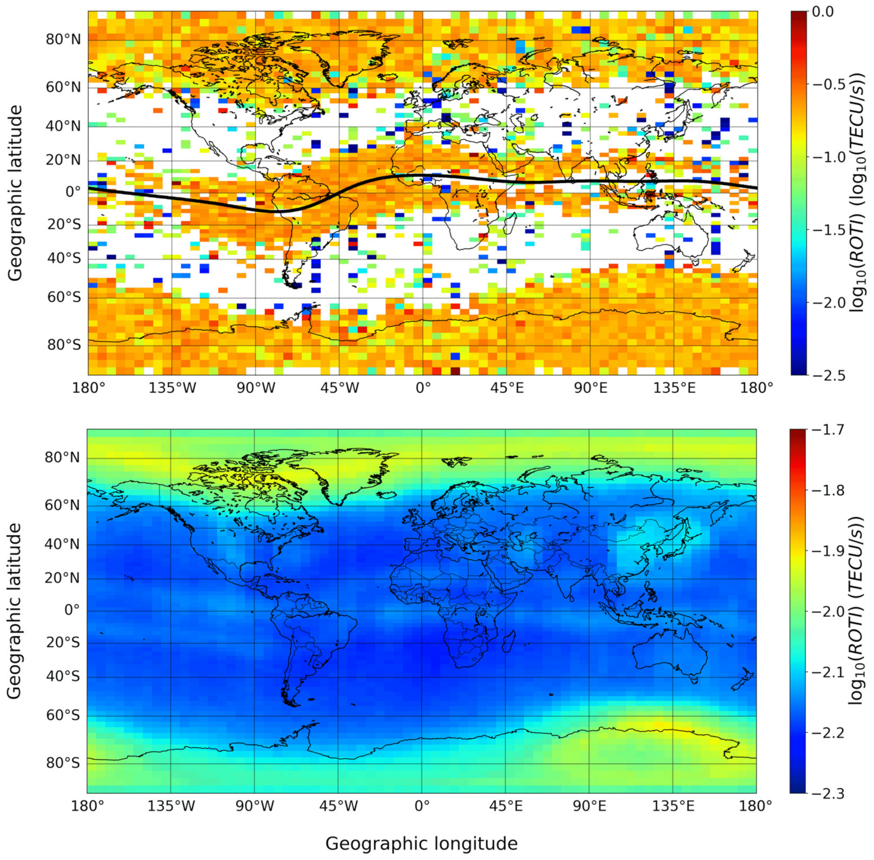
2.2. Ionospheric Indices: RODI and ROTI

By means of Ne and TEC measured time series, it is possible to calculate indices, like RODI and ROTI, characterizing their fluctuations at different spatial and temporal scales. The Swarm constellation, due to its orbit configuration and to the high sampling rate of its measurements, is particularly suited for the calculation of these indices. Several studies, exploiting Swarm data, have used these indices to get very good results about the topside ionospheric dynamics characterizing the high latitudes [22,23], as well as the low latitudes [13,24,25].

2.2.1. RODI

RODI values [26] can be obtained according to the procedure recently proposed by Pignalberi [27] through his TITIPy (Topside Ionosphere Turbulence Indices with Python) tool.

Specifically, the rate of change of electron density (ROD) is the time derivative of the electron density calculated along the satellite’s orbit using a 1st order finite difference scheme. Ne values measured by LPs onboard Swarm satellites in principle are continuous time series; however, missing measurements are possible. By indexing with k the contiguous measured values, the kth ROD value is defined as

$${\mathrm{ROD}}_k=\frac{N{\mathrm{e}}_{k+1}-N{\mathrm{e}}_k}{t_{k+1}-t_k},$$

(1)

where Ne_k is the electron density measured at time t_k. ROD values are calculated only for time consecutive measurements, that is, when the condition (t_k+1 − t_k) = δt = 0.5 s is met. Then, the kth RODI value is calculated as the standard deviation of ROD_k in a window of N = 2j + 1 elements, i.e.,

$${\mathrm{RODI}}_k=\sqrt{\frac{1}{2j}{\displaystyle \sum _{i=-j}^j{\left|{\mathrm{ROD}}_{k+i}-{\overline{\mathrm{ROD}}}_k\right|}^2}},$$

(2)

where ROD_k+i are the ROD values falling inside the window centered at the index k, whose width is N = (2j + 1), and ${\overline{\mathrm{ROD}}}_k$ is

$${\overline{\mathrm{ROD}}}_k=\frac{1}{2j+1}{\displaystyle \sum _{i=-j}^j{\mathrm{ROD}}_{k+i}}.$$

(3)

The choice of the width of the window used is crucial for the detection of fluctuations of different spatial and temporal scales. A good compromise is to select a 10-s window, as was done for instance by Jin et al. [22] and De Michelis et al. [23], which is precisely the width used in this study. This means that j = 10 and (at most) 21 values are used for RODI calculation.

RODI value is calculated only when at least half of the values are present in the window; otherwise, the corresponding value is considered not statistically significant and discarded. Then, in our case where Δt = 10 s and δt = 0.5 s, at least 11 ROD values are needed to start calculating the index.

2.2.2. ROTI

ROTI value [28] is calculated as RODI but considering TEC values in place of Ne values. However, while for each instant of time a single value of Ne is available, several TEC values can be available, because Swarm satellites can track up to eight GPS satellites simultaneously.

Specifically, the rate of change of TEC (ROT) is the time derivative of TEC calculated along the path between a Swarm satellite and a specific GPS satellite. For the sake of simplicity, in the following, we simply refer to TEC values, having in mind that both slant TEC (sTEC) and vertical TEC (vTEC) values can be used in the ROT calculation. In this study, we use absolute sTEC values, then

$${\mathrm{ROT}}_k^s=\frac{{\mathrm{TEC}}_{k+1}^s-{\mathrm{TEC}}_k^s}{t_{k+1}-t_k},$$

(4)

where s is the index running on the GPS satellites in view, identified by their Pseudo Random Noise (PRN) number. The kth ROTI value, for the GPS satellite s, is calculated as

$${\mathrm{ROTI}}_k^s=\sqrt{\frac{1}{2j}{\displaystyle \sum _{i=-j}^j{\left|{\mathrm{ROT}}_{k+i}^s-\overline{{\mathrm{ROT}}_k^s}\right|}^2}},$$

(5)

with

$$\overline{{\mathrm{ROT}}_k^s}=\frac{1}{2j+1}{\displaystyle \sum _{i=-j}^j{\mathrm{ROT}}_{k+i}^s}.$$

(6)

The window used for ROTI calculation is as wide as that used for RODI calculation.

2.3. GPS Loss of Lock Identification Methodology

In our work, the GPS LoL is identified directly from the L2 sTEC time series calculated from ambiguity-corrected carrier phase observations, performed on L₁ and L₂ signals at frequencies that are respectively equal to 1575.42 MHz and 1227.60 MHz, contained in the receiver-independent exchange files generated by the POD antennas [20]. So, when L₁ or L₂ (or both) are unavailable, the corresponding sTEC value cannot be calculated. This can happen for two reasons: (1) when the GPS satellite is outside the POD antenna field of view; or (2) when a LoL is ongoing. In this work, LoL events are identified by looking for interruptions in the sTEC time series for a specific GPS satellite (identified by the corresponding PRN) following a 4-step procedure:

• sTEC time series of each specific GPS satellite (then, of each specific PRN) are extracted from the L2 TEC data files (which contain data of all the 32 GPS satellites);
• From the sTEC time series of each specific PRN, we identify the segments of orbit for which the GPS satellite is in the field of view;
• For each of these segments of orbit, interruptions in the sTEC time series ranging from 1 to 1200 s are identified. The choice of this range guarantees that the identified interruptions are actually LoL and not due to the fact that the satellite has gone out of the field of view. This means that if, for instance, a LoL begins just before the satellite is going outside the POD field of view, this event will not be considered in our dataset;
• Steps 1–3 loop for each of the 32 GPS satellites (then, for each PRN).

An example of a GPS LoL is given in Figure 1 for an event recorded by Swarm A on 17 March 2015, during the development of the well-known St. Patrick storm. Specifically, the event represented in Figure 1 relates to PRN = 9, that was in the Swarm A field of view between 13:46:35 and 14:06:50 universal time (UT) (ascending orbit), and is identified by the interruption in the sTEC time series. Measured sTEC values, and calculated RODI and ROTI values, are represented in geographic coordinates, and as plots latitude vs. value. RODI values are obtained through (1)–(3) from Ne measurements, and ROTI values are those calculated by applying (4)–(6) to PRN = 9 sTEC measurements. By looking at sTEC panels, it is clear how sTEC increases from South to North until the time series is interrupted (between dashed magenta curves) and then reappears after a definite time interval, whose duration in this case was of 191 s. The duration of the LoL event is calculated considering the difference between the timestamps corresponding to the magenta curves in Figure 1. The same behavior is also shown by ROTI values that are derived from sTEC. A quite similar behavior is displayed also by RODI values, with the difference that RODI can be calculated also during a LoL event, if Ne data are available and not flagged.

The most important thing to notice is that both ROTI and RODI show an abrupt increase before the GPS signal is lost, and then they are both by far lower when the GPS signal reappears (the scale of both ROTI and RODI in Figure 1 is logarithmic).

Since RODI is an in situ index, being derived by in situ Ne values, while ROTI has no simple spatial characterization, being associated with the path linking Swarm and GPS satellites, the association of RODI and ROTI values to a specific LoL event is tricky. In fact, a LoL event is due to an ionospheric irregularity whose exact spatial location cannot be identified and depends on the geometric configuration of Swarm and GPS satellites. In Pignalberi [27], sTEC and corresponding ROTI values are associated with the Ionospheric Pierce Point (IPP), that is, the point where the link path between GPS and Swarm satellites pierces the spherical thin shell located 400 km above the Swarm satellite orbit. Depending on the elevation and azimuth angles between Swarm and GPS satellites, the IPP location can differ to some degrees in both latitude and longitude from the Swarm one, and this spatial difference results in a time difference between RODI and ROTI values. For these reasons, in this work, RODI and ROTI values associated with a specific LoL event will be the corresponding maximum values in a 10-s wide window centered at the LoL start timestamp (that in Figure 1 is the timestamp corresponding to the lower magenta curve).

The methodology just described has been applied to the dataset of POD sTEC data recorded by Swarm A, B, and C from 2 December 2013 to 31 December 2020. In this way, it has been possible to identify a number of LoL equal to 16,146 for Swarm A, 12,593 for Swarm B, and 15,992 for Swarm C. From here on, we talk always in terms of the cumulative dataset of LoL obtained from all the three satellites of the Swarm constellation.

Figure 2 shows the distribution of the duration (in seconds), between 1 and 100 s, of the identified LoL events. The percentage of events whose duration is greater than 100 s is less than 5.5%. The largest fraction of LoL is made up of events whose duration is of 18 s (about 29% of the total) and 1 s (about 24% of the total). The other bins are unevenly populated. This distribution is consistent with that found by Xiong et al. [14], who analyzed data from December 2013 to November 2016.

We investigated the reliability of very short LoL events. Specifically, we tried to verify whether LoL of 1 s are real or most likely due to hardware outages. To this aim, we plotted in geographic coordinates the LoL occurrences within each bin, for the following two cases:

(1)

Considering all the 44,731 LoL (top panel of Figure 3);

(2)

Discarding the 10,727 LoL whose duration is 1 s (bottom panel of Figure 3).

This comparison shows that discarding LoL of 1 s allows to eliminate most of the events located at mid latitudes, which are somewhat unexpected, not affecting at all the patterns characterizing both low and high latitudes. In virtue of this result, the analyses that is shown in Section 3 is based on LoL events whose duration is greater than 1 s.

3. Results and Discussion

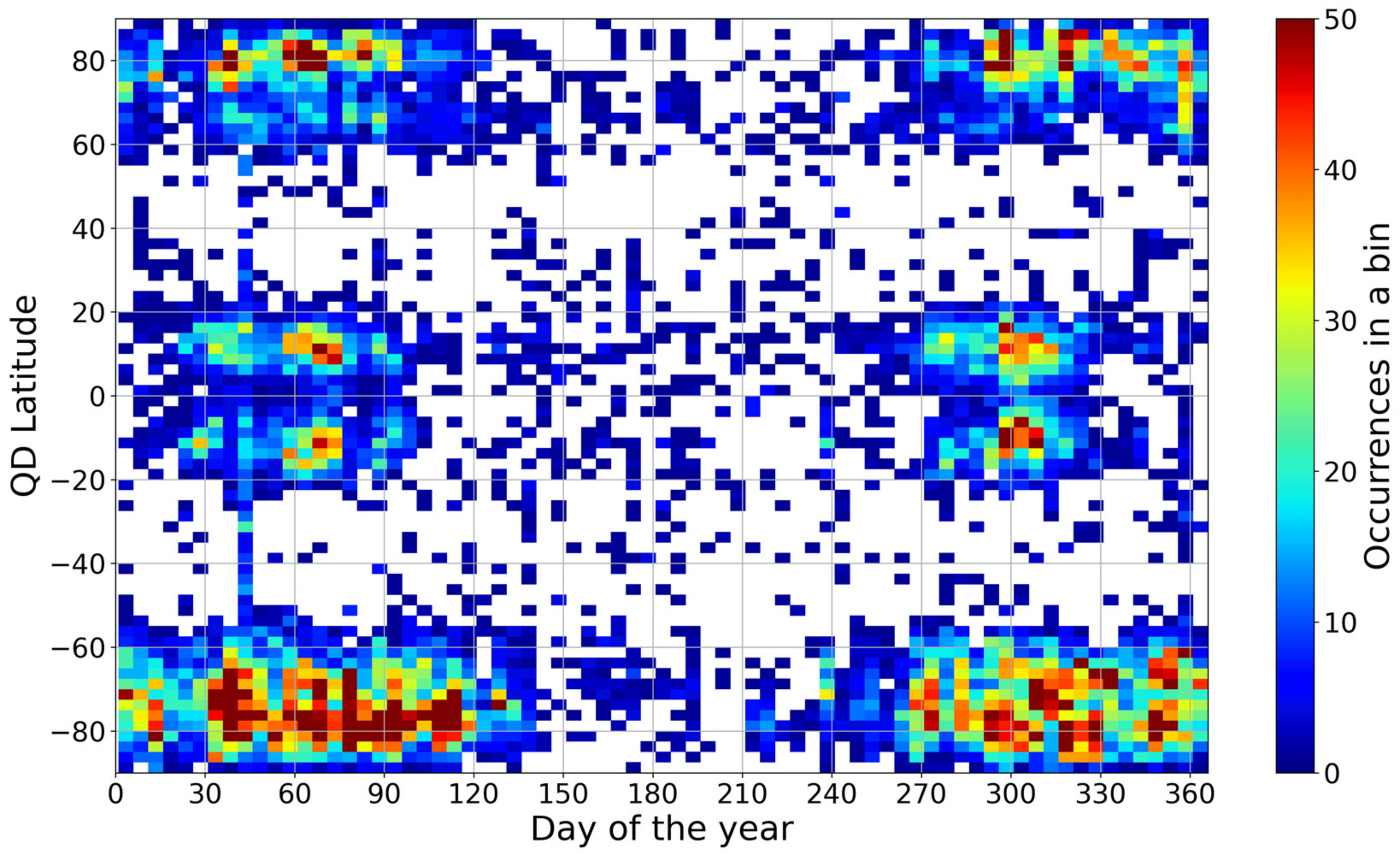
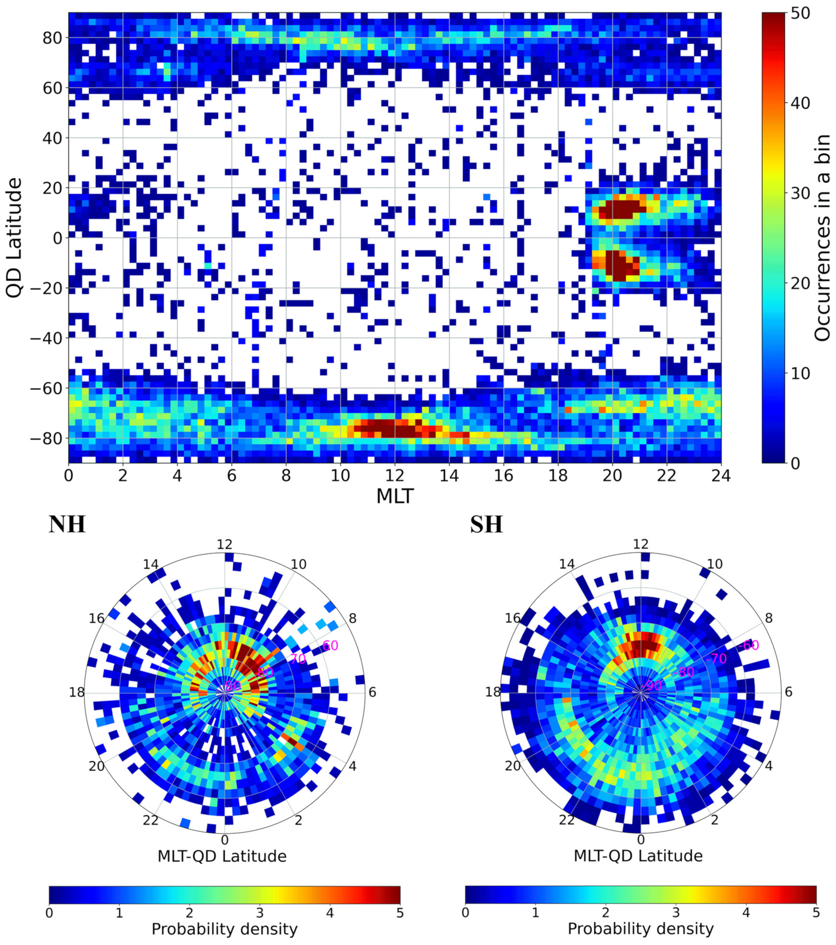
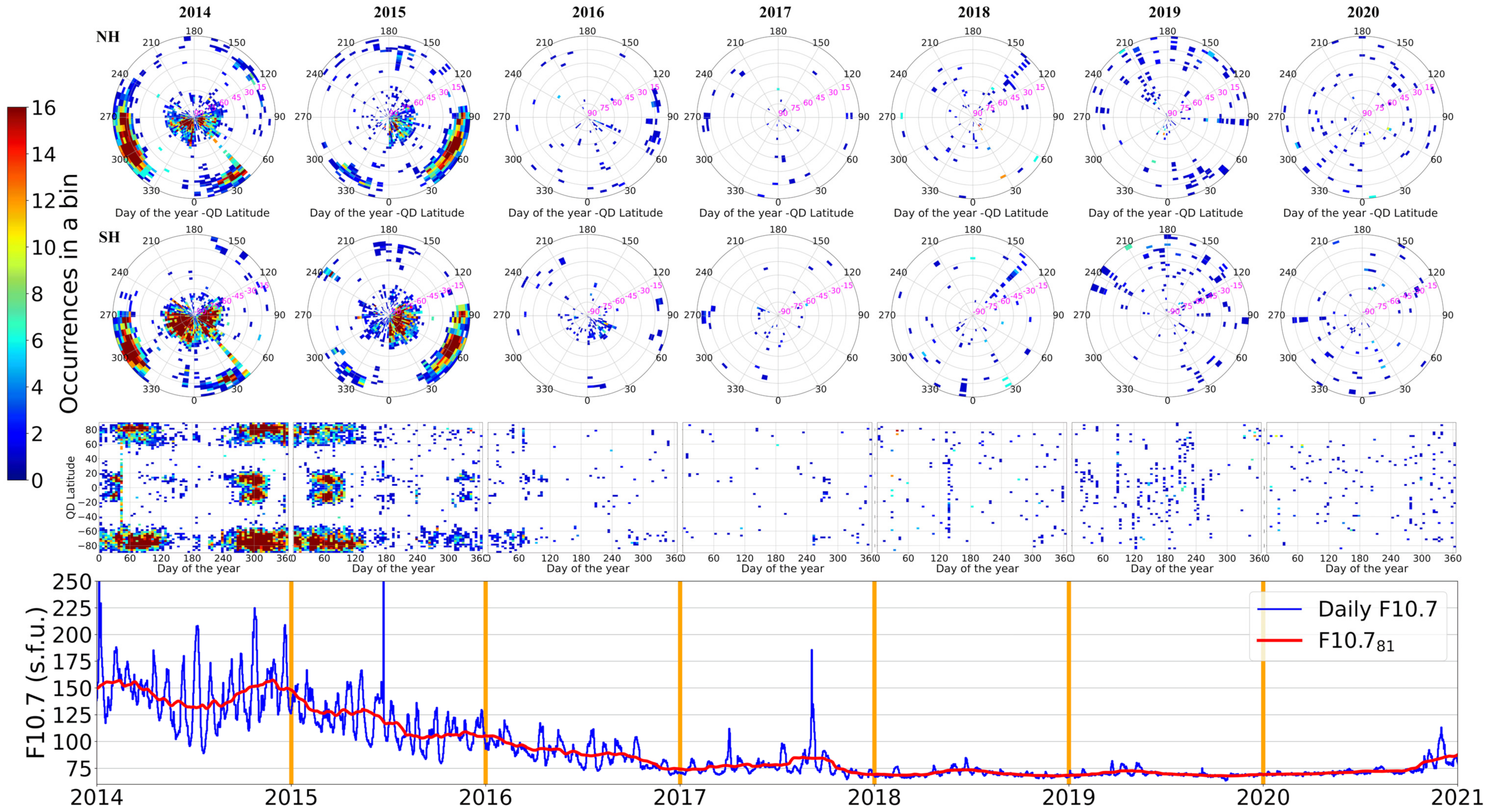
3.1. Loss of Lock Occurrence Distribution

This section discusses the distribution of the identified GPS LoL events as a function of different variables to highlight their spatial, diurnal, seasonal, and solar activity features.

Figure 3 shows the geographical distribution of LoL occurrences in bins that are 2.5°-wide in latitude and 5.0°-wide in longitude. Most of the LoL events are not randomly distributed, follow a well-defined structure, and maximize along the crests of the EIA at low latitudes, and inside the auroral oval at high latitudes, in both hemispheres.

LoL events at low latitudes have to be ascribed mainly to the generation of EPBs [6], a phenomenon that, due to the peculiar joint geometric configuration of the geomagnetic field and the equatorial zonal electric field, is more frequent at equatorial and low latitudes in the dusk–midnight sector, e.g., [29,30,31,32]. EPBs are characterized by different shapes and sizes, their lifetime ranges from a few minutes to several hours, and can seriously compromise the quality of radio signals, e.g., [33,34]. Recently, De Michelis et al. [24], using data from the ESA Swarm mission, have highlighted the turbulent nature of EPBs, suggesting at the same time a link between the scaling features of electron density fluctuations characterizing EPBs and RODI.

Considering the strong link between the equatorial plasma density irregularities and LoL events, we can suggest that the low-latitude maximum occurrence of LoL between about 70° W and 10° E of longitude has to be ascribed to both the longitudinal variation of the vertical plasma drift, and the alignment between the sunset terminator and the geomagnetic field [35]. The latter holds, taking into account that, at low latitudes, most of the plasma irregularities form in the evening sector. There is in fact a general agreement about the higher occurrence of EPBs locations where the dusk terminator is parallel to the magnetic meridian [36], a condition met in this particular longitudinal sector. Tsunoda [37] was the first who suggested that this longitudinal variation could be explained in terms of the flux tube integrated Pedersen conductivity gradients near the dusk terminator. According to Tsunoda [37], flux tubes with declinations aligning with the solar terminator facilitate the onset of the Rayleigh–Taylor (RT) instability and the onset of turbulent irregularities.

Concerning the longitudinal variability of the vertical drift, it is worth highlighting that Abdu et al. [38] and Saito and Maruyama [39] showed that there are specific longitudinal sectors, like the Southeast Asian ones, where thermospheric meridional trans-equatorial winds decrease the effect of the pre-reversal enhancement (PRE), with a consequent suppression of EPBs.

There are also studies that, in order to justify the different low-latitude longitudinal occurrence of EPBs, suggest the importance of two additional phenomena: atmospheric gravity waves that would modulate the ionospheric instabilities trigger mechanisms, e.g., [40,41]; and the South Atlantic Anomaly that would enhance the vertical drift due to the low magnetic field [42].

With regard to the high latitudes, from a longitudinal point of view, the distribution of LoL is more uniform than that at low latitudes, and confined inside the auroral oval. The auroral oval is in fact associated with significant particle precipitations and field-aligned currents from the magnetosphere, both providing the necessary energy for the development of ionospheric irregularities [43,44,45,46].

The more uniform longitudinal high-latitude distribution of LoL, if compared to the low-latitude one, has to be ascribed to the fact that the types of irregularities characterizing the high latitudes are many (polar cap patches, auroral blobs, the equatorward wall of the ionospheric trough, polar holes, and auroral cavities), located everywhere (in the dayside cusp, in the polar cap, and in the nightside auroral oval), and due to different plasma processes (the Kelvin–Helmholtz instability, the gradient drift instability, the large-scale plasma convection, the high-speed plasma convection, and the ion frictional heating) [23,47,48,49,50]. The maximum occurrence from 70° E to 180° E of geographic longitude characterizing the Southern hemisphere (SH) can be understood recalling that the geographical coordinates of the South magnetic pole are about 64.3° S and 136.6° E. So, those bins showing a high occurrence of LoL have to be thought around the South magnetic pole and inside the polar cap.

Figure 4 shows the distribution of LoL occurrences as a function of the Quasi-Dipole (QD) latitude [51] and the day of the year, in bins 2.5°-wide in QD latitude and 5-wide in days. Again, it is clear how LoL events are symmetric with respect to the magnetic equator. At low latitudes they cluster around equinoxes, while at high latitudes their occurrence is bounded between about September and May. For all latitudes, the minimum occurrence of LoL is in June, July, and August, independently of the season.

The reason of the clustering around equinoxes at low latitudes has to be found again in the alignment between the solar terminator and the geomagnetic flux tubes [35,37], a condition that is satisfied especially during equinoxes. Moreover, equinoxes are characterized by a more ionized ionosphere, a phenomenon which is known as the semiannual anomaly, e.g., [52]. This causes an increase of the equatorial zonal electric field and, around sunset, a reinforcement of the PRE, with a consequent strengthening of the vertical plasma drift. This creates a favorable environment for the RT instability, which leads to the development of EPBs, e.g., [53]. Fejer et al. [54] have done one of the first studies showing the positive correlation between the strength of PRE and the EPBs occurrence. Scherliess and Fejer [55], on the other hand, showed that eastward electric fields are more intense near the west coast of South America during March and April, which supports also the geographical distribution displayed in Figure 3. Recent works by Cai et al. [56] and Karan et al. [57], based on Global-scale Observation of Limb and Disk mission data, have given interesting insights about the South American sector in terms of the EIA hemispheric asymmetry and EPB zonal drift velocities. Furthermore, additional works by Gentile et al. [58] and Lee et al. [59] support the clustering of LoL around equinoxes. The former, using Defense Meteorological Satellite Program observations, has shown that EPBs occur most frequently around equinoxes. The latter found that the most suitable conditions for the development of EPBs, due to the interlink between the PRE and the asymmetry of EIA, occur just in the equinoctial months.

The LoL distribution characterizing the high latitudes is consistent with the seasonal trend reflecting that of polar cap patches, both in the Northern hemisphere (NH), e.g., [21,60] and in the SH [61], and that of ground-based scintillations, e.g., [62,63]. In addition, Bjoland et al. [50], using data from the European Incoherent Scatter Svalbard Radar, found that electron density depletions seem to be clearer during equinox and winter, for moderate and high solar activity, than during the rest of the year. This seasonal trend can be explained in the NH in terms of the effect of solar EUV radiation that during summer ionizes the E region, which may significantly short-circuit the F-region irregularities. Instead, in the SH this explanation can no longer be considered valid to justify the clear damping of irregularities between June and August, and other mechanisms should be invoked.

This non-seasonality characterizing the high-latitude LoL occurrence could be somehow linked to the ionospheric annual anomaly. The annual anomaly is related to the observation that, taking the world as a whole, the overall level of the maximum of electron density appears greater in December than in June, e.g., [64,65,66]. Although it has been known for more than 80 years [67], this electron density asymmetry is still unexplained. In principle, the simplest explanation of this anomaly would relate to the shape of the Earth’s orbit and, in the first place, could be ascribed to the variation of the Sun–Earth distance. The electron density annual asymmetry between solstices is, however, of about 30% and greatly exceeds the ionization rate asymmetry due to the annual variation of Sun–Earth distance which is approximately equal to 7% [68]. This is a feature that needs further and more specific studies that are out of the scope of the paper.

Figure 5 shows the distribution of LoL occurrences as a function of the QD latitude and Magnetic Local Time (MLT), in bins 2.5° and 15 min wide, respectively, in QD latitude and MLT, both as global and polar projection. Specifically, the polar projections show the probability density, just to better highlight which are the regions where the LoL occurrence maximizes. As expected, at low latitudes the events cluster between 19 and 23 MLT, the time window for which EPBs are most likely to occur, e.g., [69,70].

Differently, at high latitudes the diurnal distribution of LoL is more homogeneous, with maxima located around the local noon and in the nightside sector, mainly between 18 and 00 MLT. This is rather expected because, contrary to low latitudes, at high latitudes the ionospheric irregularities do not show a preferential time window to occur. They take place indifferently in the sub-auroral regions, in the dayside cusp, in the polar cap, as well as in the nightside auroral oval and ionospheric trough, e.g., [43,50,71,72]. Maxima related to the local noon are linked to the irregularities characterizing the dayside cusp, e.g., [73,74], while those related to the nightside sector are related to the irregularities characterizing the nightside auroral oval dynamics, e.g., [74,75].

Figure 6 shows the LoL occurrences for each year separately, from 2014 to 2020, as a function of the QD latitude and the day of the year. The bottom panel of the figure also shows the daily values of solar index F_10.7 and the corresponding 81-days running mean. F_10.7 is the solar radio flux at 10.7 cm wavelength (2800 MHz) [76] and the corresponding data have been downloaded at the National Aeronautics and Space Administration OMNIWeb Data Explorer website (https://omniweb.gsfc.nasa.gov/form/dx1.html, accessed on 31 May 2021). Figure 6 shows an evident dependence of the LoL occurrence on solar activity. In fact, LoL events maximize in 2014 and 2015, when solar activity is maximum, and they practically disappear afterwards. This confirms the findings of previous studies [35,61,77,78], namely, that ionospheric irregularities, independently of latitude, are directly proportional to solar activity and, thus, consequent phenomena such as LoL. On the other hand, for high solar activity, the physical processes at the base of the irregularities formation, like for instance the equatorial zonal electric field at low latitudes and particle precipitations at high latitudes, are much more intense, e.g., [53,79,80].

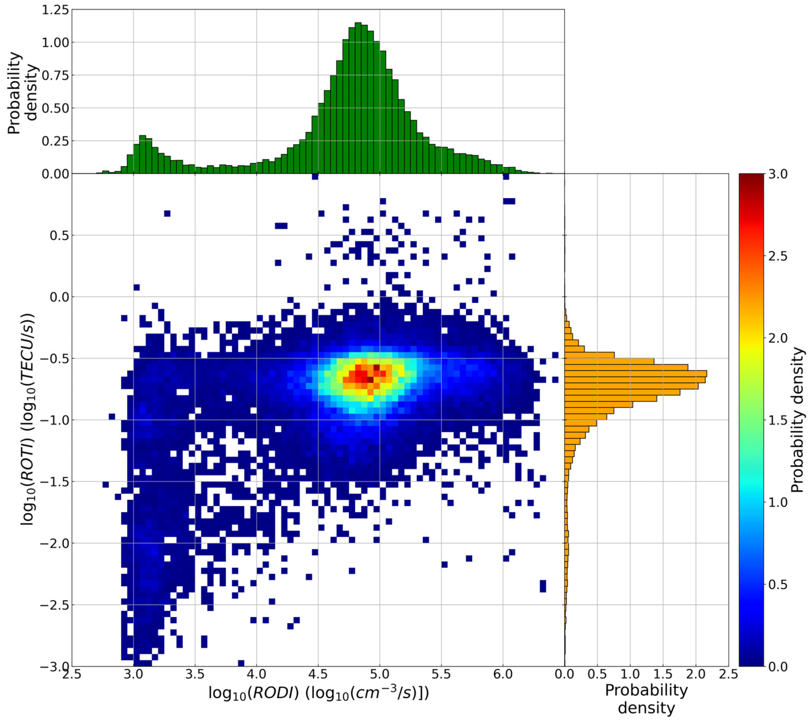
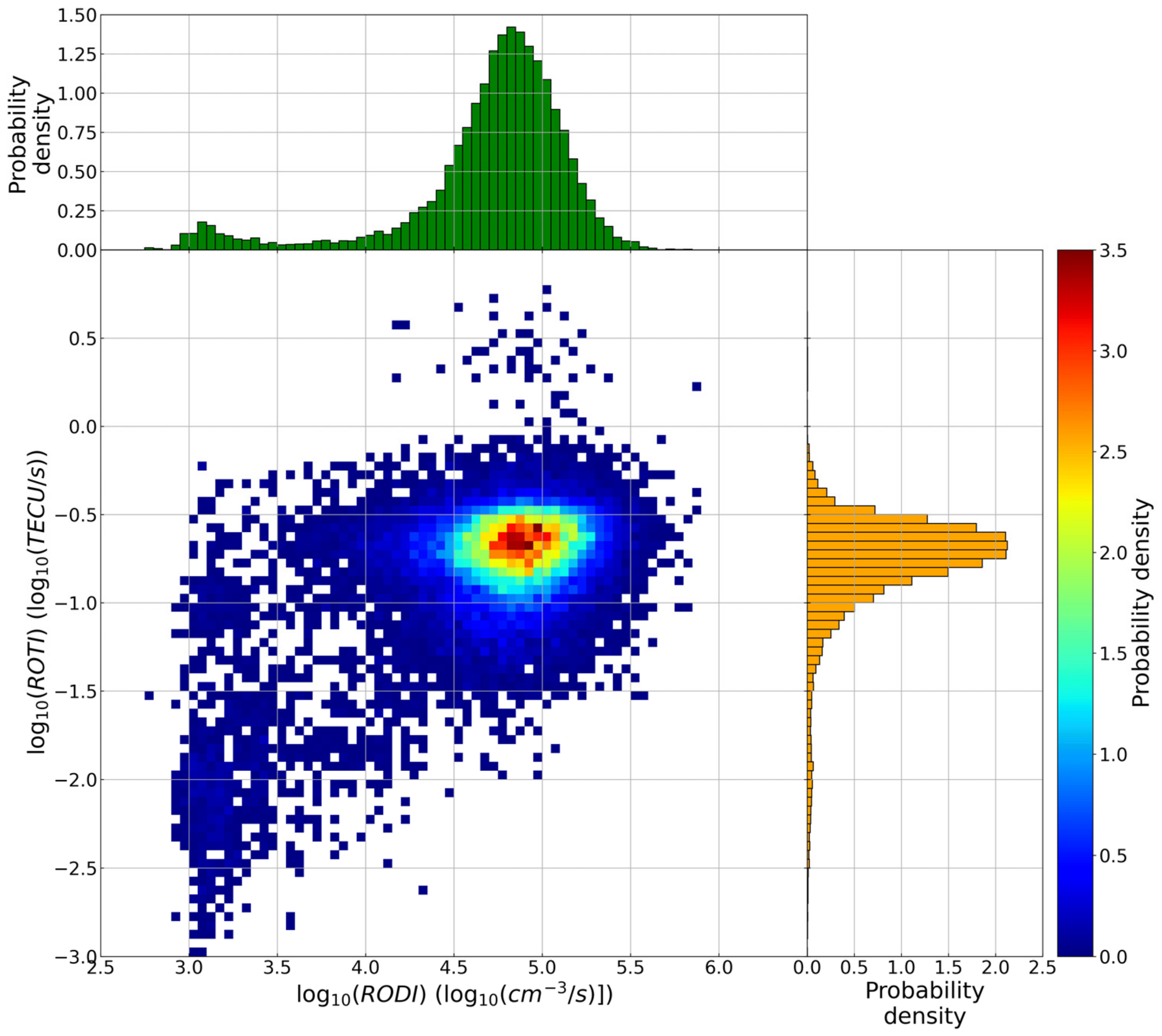
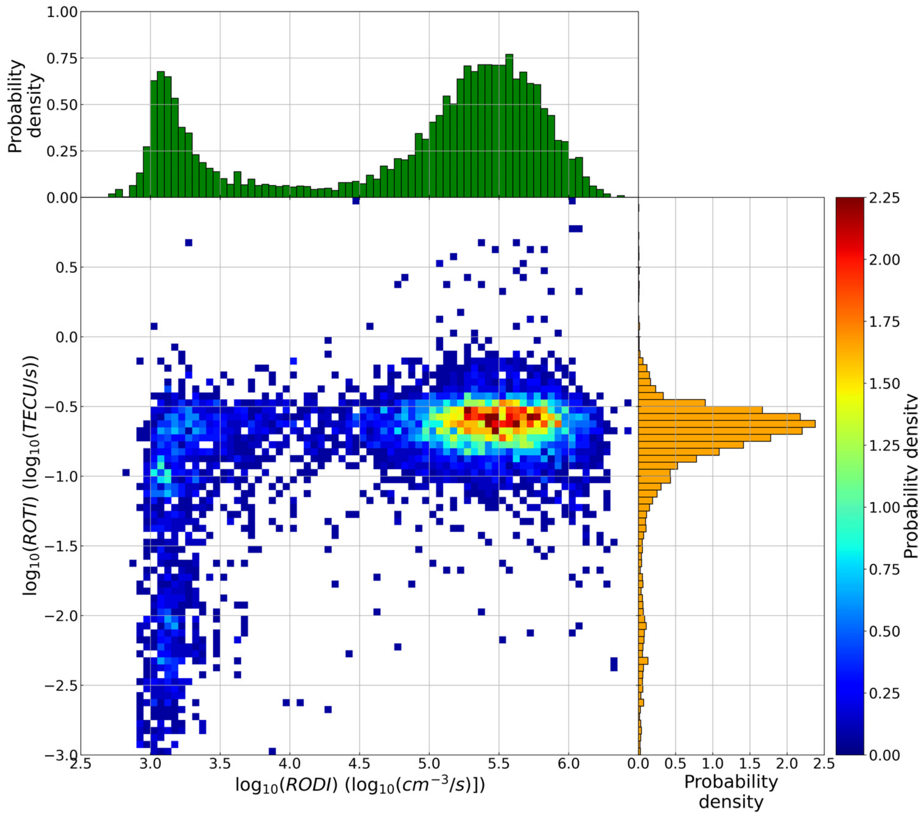
3.2. RODI and ROTI Values at GPS Loss of Lock

As previously shown in Figure 3, Figure 4 and Figure 5, the LoL distribution presents a high-latitude asymmetry between North and South, with a higher occurrence characterizing the SH than the NH. The same asymmetry was observed analyzing RODI by Jin et al. [22] and De Michelis et al. [23], who found that this is more intense in the SH than in the NH. Jin et al. [22] also found that in the SH the distribution of high values of RODI extends over a larger area than in the NH, which reflects well the LoL distribution shown for instance in Figure 3. According to this, following the procedure described in Section 2.3, we show the binned median values of RODI and ROTI values calculated during LoL events.

The top panel of Figure 7 is equivalent to the bottom panel of Figure 3, but in this case, what is represented within each bin is no longer the LoL occurrence but the median of RODI values corresponding to all LoL events falling in that bin. The dataset, the binning procedure, as well as the graphical representation of Figure 7 are the same that have been applied to obtain Figure 3. The figure shows that low-latitude RODI values are higher than high-latitude ones. The values in a log₁₀ scale range between 5 and 6 (then, between 10⁵ and 10⁶ cm⁻³/s) at low latitudes, and between 4.5 and 5.5 (then, between 10^4.5 and 10^5.5 cm⁻³/s) at high latitudes. These values are rather consistent with those found by De Michelis et al. [24,81], who investigated the properties of electron density fluctuations in terms of the first- and second-order scaling exponents and of an intermittency coefficient. This suggests that at the base of LoL events most likely there are processes of turbulent nature. It is also important to point out that the RODI values found are by far higher than those, ranging in a log₁₀ scale between 2.9 and 3.8 (then, between 10^2.9 and 10^3.8 cm⁻³/s), obtained considering all RODI values for the period December 2013–December 2020, and not only those corresponding to a LoL event, as highlighted by the bottom panel of Figure 7.

Figures similar to Figure 7, but concerning seasonal and QD latitude–MLT distributions similarly to what has been shown in Figure 4 and Figure 5 for LoL events, are visible in the Supplementary Materials as Figures S1 and S2.

Figure 8 is equivalent to Figure 7 but, in this case, what is represented is the median of ROTI values. In the top panel of Figure 8, the median within each bin is calculated considering only ROTI values corresponding to LoL events and, differently from RODI, the obtained values are similar for low and high latitudes. Again, however, it is important to highlight how these values are by far higher than those displayed in the bottom panel of Figure 8, for which the median within each bin is calculated considering all ROTI values recorded from December 2013 to December 2020, and not only those corresponding to a LoL event. In a log₁₀ scale the values in the top panel of Figure 8 range between −1.1 and −0.3 (then, between 10^−1.1 and 10^−0.3 TECU/s), while those in the bottom panel of Figure 8 range between −2.1 and −1.9 (then, between 10^−2.1 and 10^−1.9 TECU/s). It is the intention of the authors to try to investigate also the properties of the TEC fluctuations, similarly to what was done for the electron density [24,77], to strengthen the assumption that at the base of a LoL event there are processes of turbulent nature.

Figures similar to Figure 8, but concerning seasonal and QD latitude–MLT distributions similarly to what has been shown in Figure 4 and Figure 5 for LoL events, are visible in the Supplementary Materials as Figures S3 and S4. In the Supplementary Materials, the reader can also find corresponding RODI and ROTI versions of Figure 6 as Figures S5 and S6.

Figure 7 and Figure 8 highlight the fact that, in coincidence with the occurrence of a LoL event, there are high values of both RODI and ROTI, which are much higher than the background, as also highlighted by Figure 1. This means that a LoL event is most likely to occur inside regions characterized by large electron density gradients. From this perspective, with the aim of understanding if there is any value of RODI and ROTI at which it is possible to say that a LoL event has the greatest probability of occurrence, Figure 9, Figure 10 and Figure 11 show the joint probability density distribution between the values of RODI and ROTI obtained in correspondence of LoL events. Figure 9 refers to all the LoL events recorded all over the globe, while Figure 10 and Figure 11 consider only LoL events recorded at |QD latitude| > 45° and |QD latitude| ≤ 45°, respectively. Figure 9 shows that there is a well-defined family ranging between 4.5 and 5.5 values of RODI and between −0.5 and −1.0 values of ROTI (we recall that both scales are in log₁₀) for which most of the events tend to cluster. This family remains practically unchanged when considering LoL events occurred at |QD latitude| > 45°, while it moves rightward when considering LoL events occurred at |QD latitude| ≤ 45°. These results follow those recently found by De Michelis et al. [81], based only on RODI values, that have showed that high and mid-low latitudes are characterized by different families of RODI values, namely, by different kinds of physical processes responsible for the ionospheric irregularities formation. Further studies are needed, involving also additional data as the magnetic and electric field ones, to try to identify what are more specifically the processes behind the occurrence of a LoL event. This could pave the way for a future possible forecast of such events.

4. Summary and Conclusions

Considering data from the ESA Swarm constellation recorded from December 2013 to December 2020, we analyzed the occurrence of GPS LoL events and characterized them in terms of RODI and ROTI. This is the first time that such an analysis, based on such a large time window, is carried out globally, encompassing half a solar cycle, from the activity peak of 2013 to the minimum of 2020. The main outcomes of the study can be summarized as follows:

• LoL events are mainly located at low and high latitudes, for both hemispheres. Specifically, at low latitudes they maximize along the EIA crests between about 70° W and 10° E of longitude;
• The high-latitude LoL occurrence is higher in the Southern hemisphere than in the Northern hemisphere. Is this asymmetry real? This is a point that needs further analyses;
• At low latitudes, LoL events cluster around equinoxes; both high and low latitudes are characterized by a minimum of occurrence in June, July, and August, independently of the season. This non-seasonality of the LoL occurrence is intriguing and deserves additional analyses;
• At low latitudes, LoL events cluster between 19 and 23 MLT, while at high latitudes the diurnal distribution of LoL is more uniform, with maxima characterizing the local noon and the nighttime sector between 18 and 00 MLT;
• LoL events strongly depend on solar activity, maximizing for years of maximum solar activity and reducing significantly for years of minimum solar activity;
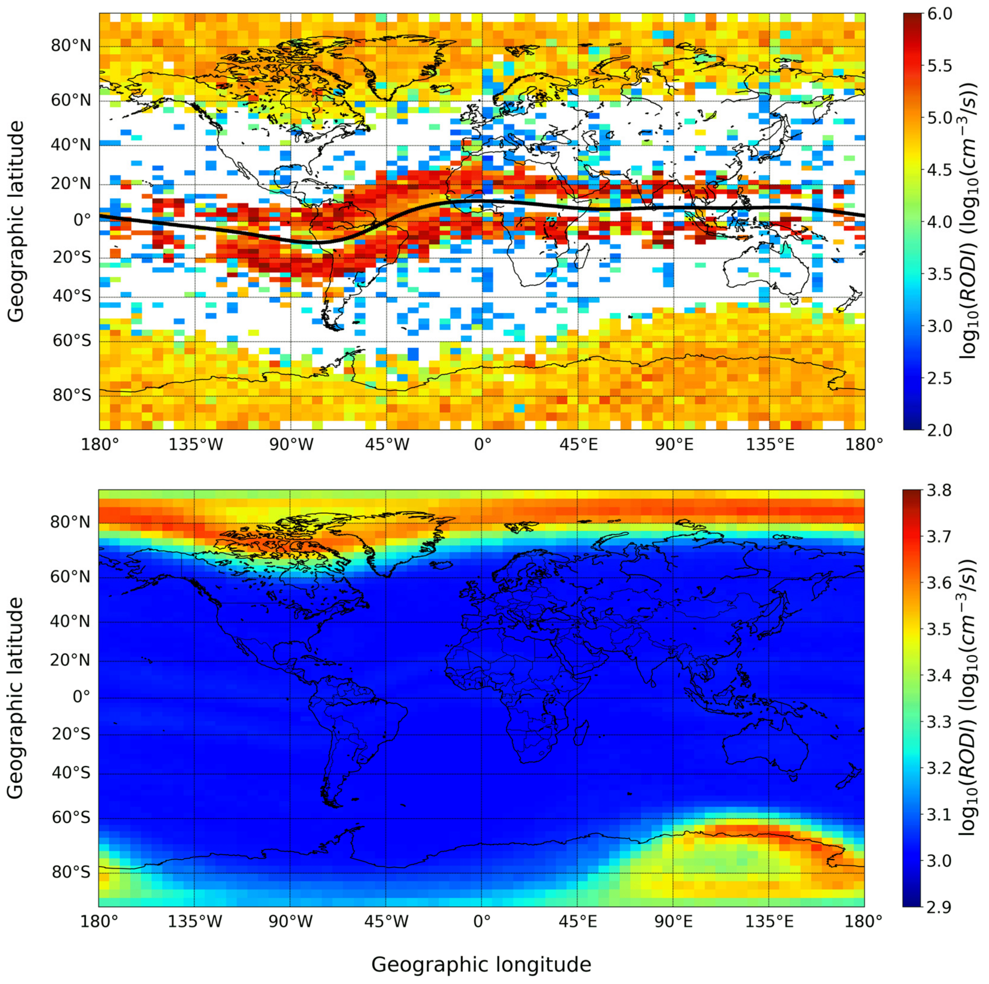
• LoL events are strictly connected with very high values of both RODI and ROTI, meaning that they are most likely to occur inside regions characterized by very large electron density gradients;
• Joint probability density distributions between RODI and ROTI values corresponding to LoL events showed that there is a well-defined family for which LoL events tend to cluster. Moreover, in terms of RODI, the values are somewhat consistent with those recently found by studies focused on the turbulent feature of ionospheric irregularities, which suggests that LoL events are likely caused by irregularities triggered by processes of turbulent nature. The position of this family changes moving from high to low latitudes. Does this movement imply that the physical processes responsible for the ionospheric irregularities formation at the base of LoL events are different? Moreover, is the second family visible for lower values of RODI (around 3) real? These questions deserve additional analyses.

Recalling that LoL events seriously degrade the accuracy of GNSS and GPS systems on which many of our infrastructures by now depend, the importance of these results can be appreciated. Trying to characterize these events in terms of ionospheric indices, as done in this work, could be valuable to lay the foundations for their possible future prediction, which would be of extreme importance in the framework of Space Weather effects mitigation.

References

1. Yeh, K.C.; Liu, C.H. Radio wave scintillations in the ionosphere. Proc. Inst. Electr. Eng. 1982, 70, 324–360. [Google Scholar] [CrossRef]
2. Cerruti, A.P.; Kintner, P.M.; Gary, D.E.; Mannucci, A.J.; Meyer, R.F.; Doherty, P.; Coster, A.J. Effect of intense December 2006 solar radio bursts on GPS receivers. Space Weather 2008, 6, S10D07. [Google Scholar] [CrossRef]
3. Alfonsi, L.; Spogli, L.; Pezzopane, M.; Romano, V.; Zuccheretti, E.; De Franceschi, G.; Cabrera, M.A.; Ezquer, R.G. Comparative analysis of spread-F signature and GPS scintillation occurrences at Tucuman, Argentina. J. Geophys. Res. Space Phys. 2013, 118, 4483–4502. [Google Scholar] [CrossRef] [Green Version]
4. Béniguel, Y. Ionospheric scintillations: Indices and modeling. Radio Sci. 2019, 54, 618–632. [Google Scholar] [CrossRef]
5. Yizengaw, E.; Groves, K. Forcing from lower thermosphere and quiet time scintillation longitudinal dependence. Space Weather 2020, 18, e2020SW002610. [Google Scholar] [CrossRef]
6. Buchert, S.; Zangerl, F.; Sust, M.; André, M.; Eriksson, A.; Wahlund, J.-E.; Opgenoorth, H. Swarm observations of equatorial electron densities and topside GPS track losses. Geophys. Res. Lett. 2015, 42, 2088–2092. [Google Scholar] [CrossRef]
7. Yue, X.; Schreiner, W.S.; Pedatella, N.M.; Kuo, Y.-H. Characterizing GPS radio occultation loss of lock due to ionospheric weather. Space Weather 2016, 14, 285–299. [Google Scholar] [CrossRef] [Green Version]
8. Liu, Y.; Fu, L.; Wang, J.; Zhang, C. Study of GNSS loss of lock characteristics under ionosphere scintillation with GNSS data at Weipa (Australia) during solar maximum phase. Sensors 2017, 17, 2205. [Google Scholar] [CrossRef] [Green Version]
9. Jin, Y.; Oksavik, K. GPS scintillations and losses of signal lock at high latitudes during the 2015 St. Patrick’s Day storm. J. Geophys. Res. 2018, 123, 7943–7957. [Google Scholar] [CrossRef]
10. Piersanti, M.; De Michelis, P.; Del Moro, D.; Tozzi, R.; Pezzopane, M.; Consolini, G.; Marcucci, M.F.; Laurenza, M.; Di Matteo, S.; Pignalberi, A.; et al. From the Sun to Earth: Effects of the 25 August 2018 geomagnetic storm. Ann. Geophys. 2020, 38, 703–724. [Google Scholar] [CrossRef]
11. Damaceno, J.G.; Bolmgren, K.; Bruno, j.; De Franceschi, G.; Mitchell, C.; Cafaro, M. GPS loss of lock statistics over Brazil during the 24th solar cycle. Adv. Space Res. 2020, 66, 219–225. [Google Scholar] [CrossRef]
12. Zhang, S.; He, L.; Wu, L. Statistical study of loss of GPS signals caused by severe and great geomagnetic storms. J. Geophys. Res. Space Phys. 2020, 125, e2019JA027749. [Google Scholar] [CrossRef]
13. Xiong, C.; Stolle, C.; Lühr, H. The Swarm satellite loss of GPS signal and its relation to ionospheric plasma irregularities. Space Weather 2016, 14, 563–577. [Google Scholar] [CrossRef]
14. Xiong, C.; Stolle, C.; Park, J. Climatology of GPS signal loss observed by Swarm satellites. Ann. Geophys. 2018, 36, 679–693. [Google Scholar] [CrossRef] [Green Version]
15. Friis-Christensen, E.; Lühr, H.; Hulot, G. Swarm: A constellation to study the Earth’s magnetic field. Earth Planets Space 2006, 58, 351–358. [Google Scholar] [CrossRef] [Green Version]
16. Knudsen, D.J.; Burchill, J.K.; Buchert, S.C.; Eriksson, A.I.; Gill, R.; Wahlund, J.-E.; Åhlen, L.; Smith, M.; Moffat, B. Thermal ion imagers and Langmuir probes in the Swarm electric field instruments. J. Geophys. Res. Space Phys. 2017, 122, 2655–2673. [Google Scholar] [CrossRef]
17. Van den IJssel, J.; Forte, B.; Montenbruck, O. Impact of Swarm GPS receiver updates on POD performance. Earth Planets Space 2016, 68, 85. [Google Scholar] [CrossRef] [Green Version]
18. Swarm L1b Product Definition. Available online: https://earth.esa.int/documents/10174/1514862/Swarm_L1b_Product_Definition (accessed on 31 May 2021).
19. Lomidze, L.; Knudsen, D.J.; Burchill, J.; Kouznetsov, A.; Buchert, S.C. Calibration and validation of Swarm plasma densities and electron temperatures using ground-based radars and satellite radio occultation measurements. Radio Sci. 2018, 53, 15–36. [Google Scholar] [CrossRef] [Green Version]
20. Swarm L2 TEC Product Description. Available online: https://earth.esa.int/eogateway/documents/20142/37627/swarm-level-2-tec-product-description.pdf/8fe7fa04-6b4f-86a7-5e4c-99bb280ccc7e (accessed on 31 May 2021).
21. Noja, M.; Stolle, C.; Park, J.; Luhr, H. Long-term analysis of ionospheric polar patches based on CHAMP TEC data. Radio Sci. 2013, 48, 289–301. [Google Scholar] [CrossRef]
22. Jin, Y.; Spicher, A.; Xiong, C.; Clausen, L.B.N.; Kervalishvili, G.; Stolle, C.; Miloch, W.J. Ionospheric plasma irregularities characterized by the Swarm satellites: Statistics at high latitudes. J. Geophys. Res. Space Phys. 2019, 124, 1262–1282. [Google Scholar] [CrossRef]
23. De Michelis, P.; Pignalberi, A.; Consolini, G.; Coco, I.; Tozzi, R.; Pezzopane, M.; Giannattasio, F.; Balasis, G. On the 2015 St. Patrick Storm Turbulent State of the Ionosphere: Hints from the Swarm Mission. J. Geophys. Res. Space Phys. 2020, 125, e2020JA027934. [Google Scholar] [CrossRef]
24. De Michelis, P.; Consolini, G.; Tozzi, R.; Pignalberi, A.; Pezzopane, M.; Coco, I.; Giannattasio, F.; Marcucci, M.F. Ionospheric Turbulence and the Equatorial Plasma Density Irregularities: Scaling Features and RODI. Remote Sens. 2021, 13, 759. [Google Scholar] [CrossRef]
25. Zakharenkova, I.; Astafyeva, E.; Cherniak, I. GPS and in situ Swarm observations of the equatorial plasma density irregularities in the topside ionosphere. Earth Planets Space 2016, 68, 120. [Google Scholar] [CrossRef] [Green Version]
26. Zakharenkova, I.; Astafyeva, E. Topside ionospheric irregularities as seen from multisatellite observations. J. Geophys. Res. Space Phys. 2015, 120, 807–824. [Google Scholar] [CrossRef] [Green Version]
27. Pignalberi, A. TITIPy: A Python tool for the calculation and mapping of topside ionosphere turbulence indices. Comp. Geosc. 2021, 148, 104675. [Google Scholar] [CrossRef]
28. Pi, X.; Mannucci, A.J.; Lindqwister, U.J.; Ho, C.M. Monitoring of global ionospheric irregularities using the worldwide GPS network. Geophys. Res. Lett. 1997, 24, 2283. [Google Scholar] [CrossRef]
29. De Rezende, L.F.C.; De Paula, E.R.; Kantor, I.J. Mapping and survey of plasma bubbles over Brazilian territory. J. Navig. 2007, 60, 69–81. [Google Scholar] [CrossRef] [Green Version]
30. Amabayo, E.B.; Jurua, E.; Cilliers, P.J.; Habarulema, J.B. Climatology of ionospheric scintillations and TEC trend over the Ugandan region. Adv. Space Res. 2014, 53, 734–743. [Google Scholar] [CrossRef]
31. Mungufeni, P.; Jurua, E.; Habarulema, J.B.; Anguma, S.K. Modelling the probability of ionospheric irregularity occurrence over African low latitude region. J. Atmos. Sol. Terr. Phys. 2015, 128, 46–57. [Google Scholar] [CrossRef]
32. Oladipo, E.A.; Xurxo, O.V.; Claudia, P.; Rodrigue, H.N.; Radicella, S.M.; Nava, B. Signature of ionospheric irregularities under different geophysical conditions on SBAS performance in the western African low-latitude region. Ann. Geophys. 2017, 35, 1–9. [Google Scholar] [CrossRef] [Green Version]
33. Paznukhov, V.V.; Carrano, C.S.; Doherty, P.H.; Groves, K.M.; Caton, R.G.; Valladares, C.E.; Seemala, G.K.; Bridgwood, C.T.; Adeniyi, J.; Amaeshi, L.L.N.; et al. Equatorial plasma bubbles and L-band scintillations in Africa during solar minimum. Ann. Geophys. 2012, 30, 675–682. [Google Scholar] [CrossRef] [Green Version]
34. Magdaleno, S.; Miguel, H.; Altadill, D.; Benito, A. Climatology characterization of equatorial plasma bubbles using GPS data. J. Space Weather Space Clim. 2017, 7, A3. [Google Scholar] [CrossRef]
35. Stolle, C.; Luhr, H.; Rother, M.; Balasis, G. Magnetic signatures of equatorial spread F as observed by the CHAMP satellite. J. Geophys. Res. 2006, 111, A02304. [Google Scholar] [CrossRef]
36. Burke, W.J.; Gentile, L.C.; Huang, C.Y.; Valladares, C.E.; Su, S.Y. Longitudinal variability of equatorial plasma bubbles observed by DMSP and ROCSAT-1. J. Geophys. Res. 2004, 109, A12301. [Google Scholar] [CrossRef]
37. Tsunoda, R.T. Control of the seasonal and longitudinal occurrence of equatorial scintillations by the longitudinal gradient in the integrated E-region Pedersen conductivity. J. Geophys. Res. 1985, 90, 447. [Google Scholar] [CrossRef]
38. Abdu, M.A.; Iyer, K.N.; de Mederios, R.T.; Batista, I.S.; Sobral, J.H.A. Thermospheric meridional wind control of equatorial spread-F and evening prereversal electric field. Geophys. Res. Lett. 2006, 33, L07106. [Google Scholar] [CrossRef] [Green Version]
39. Saito, S.; Maruyama, T. Ionospheric height variations observed by ionosondes along magnetic meridian and plasma bubble onsets. Ann. Geophys. 2006, 24, 2991–2996. [Google Scholar] [CrossRef] [Green Version]
40. Huang, C.-S.; Kelley, M.C. Nonlinear evolution of equatorial spread F: 2. Gravity wave seeding of Rayleigh-Taylor instability. J. Geophys. Res. 1996, 101, 293–302. [Google Scholar] [CrossRef]
41. McClure, J.P.; Singh, S.; Bamgboye, D.K.; Johnson, F.S.; Kil, H. Occurrence of equatorial F region irregularities: Evidence for tropospheric seeding. J. Geophys. Res. 1998, 103, 29119–29135. [Google Scholar] [CrossRef]
42. Huang, C.Y.; Burke, W.J.; Machuzak, J.S.; Gentile, L.C.; Sultan, P.J. DMSP observations of equatorial plasma bubbles in the topside ionosphere near solar maximum. J. Geophys. Res. 2001, 106, 8131. [Google Scholar] [CrossRef]
43. Tsunoda, R.T. High-latitude F-region irregularities: A review and synthesis. Rev. Geophys. 1988, 26, 719–760. [Google Scholar] [CrossRef] [Green Version]
44. Basu, S.; Mackenzie, E.; Coley, W.R.; Sharber, J.R.; Hoegy, W.R. Plasma structuring by the gradient drift instability at high-latitudes and comparison with velocity shear driven processes. J. Geophys. Res. 1990, 95, 7799–7818. [Google Scholar] [CrossRef]
45. Carlson, H. C The dark polar ionosphere: Progress and future challenges. Radio Sci. 1994, 29, 157–165. [Google Scholar] [CrossRef]
46. Clausen, L.B.N.; Moen, J.I.; Hosokawa, K.; Holmes, J.M. GPS scintillations in the high latitudes during periods of dayside and nightside reconnection. J. Geophys. Res. Space Phys. 2016, 121, 3293–3309. [Google Scholar] [CrossRef]
47. Kelley, M.C.; Vickrey, J.F.; Carlson, C.W.; Torbert, R. On the origin and spatial extent of high-latitude F region irregularities. J. Geophys. Res. 1982, 87, 4469–4475. [Google Scholar] [CrossRef]
48. Cherniak, I.; Zakharenkova, I.; Redmon, R.J. Dynamics of the high-latitude ionospheric irregularities during the 17 March 2015 St. Patrick’s Day storm: Ground-based GPS measurements. Space Weather 2015, 13, 585–597. [Google Scholar] [CrossRef]
49. Cherniak, I.; Zakharenkova, I. High-latitude ionospheric irregularities: Differences between ground-and space-based GPS measurements during the 2015 St. Patrick’s Day storm. Earth Planets Space 2016, 68, 136. [Google Scholar] [CrossRef]
50. Bjoland, L.M.; Ogawa, Y.; Løvhaug, U.P.; Lorentzen, D.A.; Hatch, S.M.; Oksavik, K. Electron density depletion region observed in the polar cap ionosphere. J. Geophys. Res. Space Phys. 2021, 126, e2020JA028432. [Google Scholar] [CrossRef]
51. Laundal, K.M.; Richmond, A.D. Magnetic Coordinate Systems. Space Sci. Rev. 2017, 206, 27. [Google Scholar] [CrossRef] [Green Version]
52. Mendillo, M.; Huang, C.-L.; Pi, X.; Rishbeth, H.; Meier, R. The global ionospheric asymmetry in total electron content. J. Atmos. Sol. Terr. Phys. 2005, 67, 1377–1387. [Google Scholar] [CrossRef]
53. Abiriga, F.; Amabayo, E.B.; Jurua, E.; Cilliers, P.J. Statistical characterization of equatorial plasma bubbles over East Africa. J. Atmos. Sol. Terr. Phys. 2020, 200, 105197. [Google Scholar] [CrossRef]
54. Fejer, B.G.; Scherliess, L.; de Paula, E.R. Effects of the vertical plasma drift velocity on the generation and evolution of equatorial spread F. J. Geophys. Res. 1999, 104, 19859–19869. [Google Scholar] [CrossRef] [Green Version]
55. Scherliess, L.; Fejer, B.G. Radar and satellite global equatorial F region vertical drift model. J. Geophys. Res. 1999, 104, 6829. [Google Scholar] [CrossRef]
56. Cai, X.; Burns, A.G.; Wang, W.; Qian, L.; Liu, J.; Solomon, S.C.; Eastes, R.W.; Daniell, R.E.; Martinis, C.R.; McClintock, W.E.; et al. Observation of postsunset OI 135.6 nm radiance enhancement over South America by the GOLD mission. J. Geophys. Res. Space Phys. 2012, 126, e2020JA028108. [Google Scholar] [CrossRef]
57. Karan, D.K.; Daniell, R.E.; England, S.L.; Martinis, C.R.; Eastes, R.W.; Burns, A.G.; McClintock, W.E. First zonal drift velocity measurement of equatorial plasma bubbles (EPBs) from a geostationary orbit using GOLD data. J. Geophys. Res. Space Phys. 2020, 125, e2020JA028173. [Google Scholar] [CrossRef]
58. Gentile, L.C.; Burke, W.J.; Roddy, P.A.; Retterer, J.M.; Tsunoda, R.T. Climatology of plasma density depletions observed by DMSP in the dawn sector. J. Geophys. Res. 2011, 116, A03321. [Google Scholar] [CrossRef]
59. Lee, C.C.; Liu, J.Y.; Reinisch, B.W.; Chen, W.S.; Chu, F.D. The effects of the prereversal drift, the EIA asymmetry, and magnetic activity on the equatorial spread F during solar maximum. Ann. Geophys. 2005, 23, 745–751. [Google Scholar] [CrossRef] [Green Version]
60. Spicher, A.; Cameron, T.; Grono, E.M.; Yakymenko, K.N.; Buchert, S.C.; Clausen, L.B.N.; Knudsen, D.J.; McWilliams, K.A.; Moen, J.I. Observation of polar cap patches and calculation of gradient drift instability growth times: A Swarm case study. Geophys. Res. Lett. 2015, 42, 201–206. [Google Scholar] [CrossRef]
61. Rodger, A.S.; Graham, A.C. Diurnal and seasonal occurrence of polar patches. Ann. Geophys. 1996, 14, 533–537. [Google Scholar] [CrossRef]
62. Prikryl, P.; Jayachandran, P.T.; Chadwick, R.; Kelly, T.D. Climatology of GPS phase scintillation at northern high latitudes for the period from 2008 to 2013. Ann. Geophys. 2015, 33, 531–545. [Google Scholar] [CrossRef] [Green Version]
63. Jin, Y.Q.; Miloch, W.J.; Moen, J.I.; Clausen, L.B.N. Solar cycle and seasonal variations of the GPS phase scintillation at high latitudes. J. Space Weather Space Clim. 2018, 8, A48. [Google Scholar] [CrossRef] [Green Version]
64. Sai Gowtam, V.; Tulasi Ram, S. Ionospheric annual anomaly—New insights to the physical mechanisms. J. Geophys. Res. Space Phys. 2017, 122, 8816–8830. [Google Scholar] [CrossRef]
65. Zeng, Z.; Burns, A.; Wang, W.; Lei, J.; Solomon, S.; Syndergaard, S.; Qian, L.; Kuo, Y.-H. Ionospheric annual asymmetry observed by the COSMIC radio occultation measurements and simulated by the TIEGCM. J. Geophys. Res. 2008, 113, A07305. [Google Scholar] [CrossRef] [Green Version]
66. Burns, A.G.; Solomon, S.C.; Wang, W.; Qian, L.; Zhang, Y.; Paxton, L.J. Daytime climatology of ionospheric NmF2 and hmF2 from COSMIC data. J. Geophys. Res. 2012, 117, A09315. [Google Scholar] [CrossRef]
67. Berkner, L.V.; Wells, H.W.; Seaton, S.L. Characteristics of the upper region of the ionosphere. J. Geophys. Res. 1936, 41, 173–184. [Google Scholar] [CrossRef]
68. Rishbeth, H.; Muller-Wodarg, I.C.F. Why is there more ionosphere in January than in July? The annual asymmetry in the F2-layer. Ann. Geophys. 2006, 24, 3293–3311. [Google Scholar] [CrossRef] [Green Version]
69. Aa, E.; Zou, S.; Eastes, R.; Karan, D.K.; Zhang, S.-R.; Erickson, P.J.; Coster, A.J. Coordinated ground-based and space-based observations of equatorial plasma bubbles. J. Geophys. Res. Space Phys. 2020, 125, e2019JA027569. [Google Scholar] [CrossRef]
70. Abdu, M.A.; Kherani, E.A.; Sousasantos, J. Role of bottom-side density gradient in the development of equatorial plasma bubble/spread F irregularities: Solar minimum and maximum conditions. J. Geophys. Res. Space Phys. 2020, 125, e2020JA027773. [Google Scholar] [CrossRef]
71. Hanuise, C. High-latitude ionospheric irregularities: A review of recent radar results. Radio Sci. 1983, 18, 1093–1121. [Google Scholar] [CrossRef]
72. Keskinen, M.J.; Ossakow, S.L. Theories of high-latitude ionospheric irregularities: A review. Radio Sci. 1983, 18, 1077–1091. [Google Scholar] [CrossRef]
73. Oksavik, K.; Moen, J.; Lester, M.; Bekkeng, T.A.; Bekkeng, J.K. In situ measurements of plasma irregularity growth in the cusp ionosphere. J. Geophys. Res. 2012, 117, A11301. [Google Scholar] [CrossRef]
74. Jin, Y.; Moen, J.I.; Oksavik, K.; Spicher, A.; Clausen, L.B.N.; Miloch, W.J. GPS scintillations associated with cusp dynamics and polar cap Patches. J. Space Weather Space Clim. 2017, 7, A23. [Google Scholar] [CrossRef]
75. van der Meeren, C.; Oksavik, K.; Lorentzen, D.A.; Rietveld, M.T.; Clausen, L.B.N. Severe and localized GNSS scintillation at the poleward edge of the nightside auroral oval during intense substorm aurora. J. Geophys. Res. Space Phys. 2015, 120, 10607–10621. [Google Scholar] [CrossRef] [Green Version]
76. Tapping, K.F. The 10.7 cm solar radio flux (F10.7). Space Weather 2013, 11, 394–406. [Google Scholar] [CrossRef]
77. Aarons, J.; Mullen, J.P.; Whitney, H.E.; Johnson, A.L.; Weber, E.J. UHF scintillation activity over polar latitudes. Geophys. Res. Lett. 1981, 8, 277–280. [Google Scholar] [CrossRef]
78. Basu, S.; Groves, K.M.; Basu, S.; Sultan, P.J. Specification and forecasting of scintillations in communication/navigation links: Current status and future plans. J. Atmos. Sol. Terr. Phys. 2002, 64, 1745–1754. [Google Scholar] [CrossRef]
79. Su, S.-Y.; Liu, C.H.; Ho, H.H.; Chao, C.K. Distribution characteristics of topside ionospheric density irregularities: Equatorial versus midlatitude regions. J. Geophys. Res. 2006, 111, A06305. [Google Scholar] [CrossRef]
80. Kotulak, K.; Zakharenkova, I.; Krankowski, A.; Cherniak, I.; Wang, N.; Fron, A. Climatology Characteristics of Ionospheric Irregularities Described with GNSS ROTI. Remote Sens. 2020, 12, 2634. [Google Scholar] [CrossRef]
81. De Michelis, P.; Consolini, G.; Pignalberi, A.; Tozzi, R.; Coco, I.; Giannattasio, F.; Pezzopane, M.; Balasis, G. Looking for a proxy of the ionospheric turbulence with Swarm data. Sci. Rep. 2021, 11, 6183. [Google Scholar] [CrossRef]
Figure 1. Example of GPS LoL event identified at around 14 UT by Swarm A during its ascending orbit between 13:46:35 and 14:06:50 UT on 17 March 2015 and related to PRN = 9. Magenta curves identify the GPS LoL duration, that in this case is of 191 s. Left, middle, and right panels refer respectively to sTEC, ROTI, and RODI. Upper panels represent the values in geographic coordinates, while the lower ones show the corresponding plots latitude vs. value. 1 TEC unit (TECU) = 1016 electrons/m2.
Remotesensing 13 02209 g001
Figure 2. Distribution of the duration (in seconds), between 1 and 100 s, for the cumulative dataset of LoL events suffered by Swarm A, B, and C, between December 2013 and December 2020. Results are given as percentage of occurrence in bins one-second wide. The total number of LoL is 44,731.
Remotesensing 13 02209 g002
Figure 3. Geographic distribution of the GPS LoL occurrence affecting Swarm A, B, and C, from December 2013 to December 2020, considering (top panel) all LoL events, independently of the duration, and (bottom panel) considering only those events whose duration is greater than 1 s. The magenta curve visible in both panels represents the magnetic equator.
Remotesensing 13 02209 g003
Figure 4. Distribution of the GPS LoL occurrence affecting Swarm A, B, and C, from December 2013 to December 2020, as a function of the QD latitude and the day of the year.
Remotesensing 13 02209 g004
Figure 5. Distribution of the GPS LoL events affecting Swarm A, B, and C, from December 2013 to December 2020, as a function of the QD latitude and MLT. (Top panel) Global projection of the occurrence. (Bottom panels) Polar projections (where the radius is the QD latitude and the azimuth angle is the MLT) for (left) the Northern hemisphere (where the QD latitude ranges from 50° to the North magnetic pole) and (right) the Southern hemisphere (where the QD latitude ranges from –50° to the South magnetic pole) of the probability density.
Remotesensing 13 02209 g005
Figure 6. Same as Figure 4 but for each year of the considered dataset, from 2014 to 2020. Polar projection (where the radius is the QD latitude and the azimuth angle is the day of the year) (first row) for the Northern hemisphere, (second row) for the Southern hemisphere, (third row) global projection, (fourth row) daily values of the F10.7 solar index (in blue) and corresponding 81-days running mean F10.781 (in red).
Remotesensing 13 02209 g006
Figure 7. (Top panel) Same as Figure 3 but for RODI values at GPS loss of lock. The black curve represents the magnetic equator. (Bottom panel) RODI median values obtained for the period December 2013–December 2020 taking into account all RODI values and not only those corresponding to a LoL event.
Remotesensing 13 02209 g007
Figure 8. Same as Figure 7 but for ROTI values.
Remotesensing 13 02209 g008
Figure 9. Joint probability density distribution of RODI and ROTI values at GPS loss of lock, independently of the QD latitude, for the period December 2013–December 2020. On the top and right panels, histograms of the probability density for RODI and ROTI are also reported.
Remotesensing 13 02209 g009
Figure 10. Same as Figure 9 but selecting only GPS LoL events occurred for |QD latitude| > 45°.
Remotesensing 13 02209 g010
Figure 11. Same as Figure 9 but selecting only GPS LoL events occurred for |QD latitude| ≤ 45°.
Remotesensing 13 02209 g011
Publisher’s Note: MDPI stays neutral with regard to jurisdictional claims in published maps and institutional affiliations.