Article

Extraction of Irrigation Signals by Using SMAP Soil Moisture Data

1
College of Hydraulic Science and Engineering, Yangzhou University, Yangzhou 225009, China
2
Key Laboratory of Virtual Geographic Environment (Nanjing Normal University), Ministry of Education, Nanjing 210046, China
3
State Key Laboratory Cultivation Base of Geographical Environment Evolution (Jiangsu Province), Nanjing 210046, China
4
Jiangsu Center for Collaborative Innovation in Geographical Information Resource Development and Application, Nanjing 210046, China
5
Department of Geography, University of Wisconsin-Madison, Madison, WI 53706, USA
*
Author to whom correspondence should be addressed.
Remote Sens. 2021, 13(11), 2142; https://doi.org/10.3390/rs13112142
Submission received: 23 April 2021 / Revised: 27 May 2021 / Accepted: 27 May 2021 / Published: 29 May 2021
(This article belongs to the Section Remote Sensing in Agriculture and Vegetation)

Abstract

:
To allow extraction of irrigation signals from satellite-derived data on soil moisture, this study describes the development of an irrigation signal extraction method that takes into account multiple environmental factors in irrigation. Firstly, the fuzzy membership functions of irrigation relating to multiple environmental factors are constructed. Then, a model is built based on the fuzzy membership functions by using operation rules of fuzzy sets, which is used to infer the relevant degree of irrigation to nonirrigation. Finally, the irrigation signals in satellite-based soil moisture data are recognized according to the relevant degree. Taking Henan Province in the North China Plain as the study area, the proposed method is used to extract irrigation signals from the SMAP Level 3 Passive Soil Moisture Product. Extracted irrigation signals from two SMAP grids are validated using daily in situ soil moisture and precipitation data, with the results showing correct identification of most of the irrigation signals. By grading the membership degree of the extracted irrigation signals, irrigation frequency maps for the 2016–2017 winter crop growth season and the 2017 summer crop growth season are obtained for Henan Province. Compared to the irrigation frequency maps with data on the annual precipitation and the annual potential evapotranspiration, the irrigation frequency maps show a spatial pattern opposite that of the annual precipitation and a spatial pattern similar to that of the annual potential evapotranspiration. It is common sense that areas with low precipitation and high evapotranspiration need more irrigation frequency and irrigation water. Thus, the spatial patterns of irrigation frequency maps are reasonable in a sense. However, it should be noted that the observed irrigation data used in the qualitative assessments are rendered less convincing by the SMAP product’s coarse resolution. Quantitative validation of extracted irrigation signals remains a significant challenge, and small-scale irrigation cannot be captured by coarse-resolution satellite-based soil moisture products. Thus, a high-resolution soil moisture product should be used to extract irrigation signals in future.

1. Introduction

Irrigation is a significant contributor to agricultural production, especially in cultivated areas that suffer from water shortages [1,2,3,4]. As a result, irrigation requires the use of vast quantities of fresh water every year. In 2000, for example, about 2600 km3 of fresh water withdrawn from surface water or groundwater was used for irrigation [5,6]. As extreme weather events increase in frequency, more freshwater will be needed for irrigation to guarantee global food supply [7,8,9]. Such extensive use of water for irrigating land surfaces has significantly affected local climates and water cycles [10,11].
Irrigation information, such as irrigation extent and irrigation timing, plays a key role in studying irrigation as well as its effects. Many researchers have tried to acquire irrigation information through remote sensing, which is less costly and time-intensive than traditional methods [12,13,14]. Optical remote sensing was first used to acquire irrigation information [15,16], usually based on the following assumptions: (1) Irrigation and fertilization are implemented simultaneously, so that crops with irrigation grow faster and flourish more than non-irrigated ones. The differences between irrigated and nonirrigated crops can be captured by optical remote sensing [17,18]. (2) Irrigation raises crop and soil moisture, and signals such as the increase of crop and soil moisture can be captured by optical remote sensing in the long-wave band [19]. Based on these assumptions, Ozdogan and Gutman [15] compared the time series green index (GI) of irrigated and nonirrigated areas and found significant differences. In addition, Chen et al. [18] reported that the time series GI of irrigated areas tends to increase sharply after precipitation or irrigation during the vegetation growth stage. Using a threshold of effective precipitation, increased GI after effective precipitation was attributed to precipitation but increased GI during a period with no effective precipitation to irrigation. However, extraction of irrigation timing and irrigation frequency is more difficult than extraction of irrigated areas through optical remote sensing owing to soils’ and crops’ complex response to irrigation [20]. Chen et al. [18] reported that GI calculated in the near-infrared band (840–880 μm) and green band (540–570 μm) was sensitive to soil moisture in arid and lightly vegetated areas, but performed poorly in wet and densely vegetated areas owing to the weak penetration offered by optical remote sensing [15,18].
Recently, several satellite-based soil moisture products based on satellite microwave remote sensing data have been made available, such as AMSR-E (Advanced Microwave Scanning Radiometer for the Earth Observing System), SMOS (Soil Moisture and Ocean Salinity), and SMAP (Soil Moisture Active & Passive). These soil moisture products can provide near-surface (i.e., 0–5 cm) soil moisture data with high precision and high time resolution [21,22,23,24]. Because irrigation increases surface soil moisture, irrigation information can theoretically be extracted from satellite-based soil moisture data. Previous studies have found that satellite-based soil moisture products can capture irrigation signals [25,26,27,28,29,30,31,32]. For example, Singh et al. [27] compared time series AMSR-E soil moisture in an irrigated area with that in a nonirrigated area in northern India and found that the peaks of time series AMSR-E soil moisture in the irrigated area exceeded those in the nonirrigated area as a result of irrigation. Similarity, Lawston et al. [28] compared the SMAP level 3 enhanced soil moisture in an irrigated area and a nonirrigated area in Sacramento Valley and found that changes in SMAP soil moisture in the irrigated area resembled those in the nonirrigated area during the rainy season (November to March), but that in the dry season (May to July), SMAP soil moisture in the irrigated area remained high through irrigation even as it decreased continuously in the nonirrigated areas. These results demonstrate that the SMAP level 3 enhanced soil moisture product can capture irrigation signals. The research mentioned confirms that soil moisture data retrieved through microwave remote sensing can capture irrigation signals, although irrigation signals cannot be extracted based on satellite-based soil moisture data. The key papers for detection/extraction of irrigation signals from satellite-based soil moisture data are summarized in Table 1.
To extract irrigation signals from satellite-based soil moisture data, Hao et al. [33] used an effective rainfall threshold of 4 mm to distinguish irrigation signals and nonirrigation signals. In his study, the increased stages in satellite-based soil moisture that have effective rainfall were identified as the irrigation signal, and increased stages in satellite-based soil moisture that have no effective rainfall were identified as the nonirrigation signal. The method proposed by Hao et al. [33] is easy to implement but cannot express the relationship between irrigation and environmental factors: Because only one environmental factor of rainfall is used to identify irrigation signals, other environmental factors, such as initial soil moisture conditions, cannot be taken into consideration. Accordingly, this study is intended to develop an irrigation signal extraction method that can take into account of multiple environmental factors relating to irrigation.

2. Basic Idea

Figure 1 shows time series SMAP soil moisture and precipitation for 2017 at one SMAP pixel. As the period in the red rectangle in Figure 1a shows, SMAP soil moisture obviously increases, but no precipitation occurs during this period. Figure 1b shows in situ soil moisture at seven sites, which increases rapidly at different times under conditions of no precipitation. Because irrigation and precipitation are the two causes of increases in soil moisture in the study area, the increase of SMAP soil moisture in red rectangle period in Figure 1a can be attributed to irrigation. The aim of this study is to extract irrigation signals such as increases in SMAP soil moisture in the red rectangle in Figure 1a.
Increases in soil moisture in farmland caused by irrigation can occur in two situations: (1) no precipitation during increases in soil moisture, so that irrigation can be concluded to have increased the soil moisture, and (2) small amounts of precipitation during increases in soil moisture, so that if initial soil moisture is low and precipitation insufficient to ease the drought, irrigation can be deemed to have been necessary. Accordingly, increases in soil moisture cannot be arbitrarily attributed to irrigation (precipitation) or vice versa, being potentially caused by both irrigation and precipitation in varying degrees. Such a gradual relationship between increases in soil moisture and impact factors (irrigation and precipitation) can be described using fuzzy logic [34,35,36].
In this study, the nonlinear relationships between irrigation necessity and multiple environmental factors are described using a set of fuzzy membership functions. A model is then built based on the fuzzy membership functions by using operation rules of fuzzy sets, which is used to recognize irrigation signals in satellite-based soil moisture.

3. Study Area and Datasets

3.1. Study Area

The study area of Henan Province is located in the southwest of the North China Plain and has an area of about 156,000 km2. The main land cover is farmland in the plain areas, with dry farmland accounting for about 78% of the total area (Figure 2a). The grids in Figure 2a indicate the locations of SMAP pixels.
Henan Province has a subtropical monsoon climate, with an annual average precipitation of 400–900 mm. Precipitation in the study area is extremely uneven temporally and spatially, being greater in the southern and western mountains and less in the north. In addition, about 80% of the precipitation is concentrated in the warm season [37]. Owing to the limited and uneven distribution of precipitation, dry farmland in the study area relies heavily on irrigation. According to statistical data from the Henan Water Resources Bulletin, about 50–70% of dry farmland requires irrigation every year (http://www.hnssw.com.cn/resources/index.jhtml). The grids in the figures indicate the locations of satellite-based soil moisture data (SMAP). Figure 2c shows the environment of in situ soil moisture sites, with management of in situ soil moisture sites the same as in farmland. Meteorological data, such as precipitation, temperature, and wind speed, are also collected at each site.

3.2. Datasets

3.2.1. Soil Moisture Datasets

(1) SMAP L3 Passive Soil Moisture Product

The SMAP mission was developed by the National Aeronautics and Space Administration (NASA). On 31 January 2015, the SMAP satellite was launched into a polar sun-synchronous orbit (descending orbit at 6:00 a.m. and ascending orbit at 6:00 p.m., local solar time), carrying an L-band radar and radiometer. Unfortunately, the radar stopped working a few months after launch because of an irrecoverable hardware failure. The radiometer that still remains provides 36 km-resolution passive observations every two to three days. SMAP’s mission is to retrieve soil moisture, with SMAP soil moisture products seemingly more accurate than other passive satellite-based soil moisture products in many places [38,39,40]. A previous study noted that the SMAP_P L3 soil moisture product performed best in the study area among three L-band satellite-based soil moisture products, including the SMAP L3 soil moisture product, the SMOS L3 soil moisture product, and the European Space Agency’s Climate Change Initiative (ESA CCI) soil moisture product [41]. Some previous studies also point out that SMAP_P product can capture irrigation signals [29,30,31]. In addition, Lawston et al. [28] and Hao et al. [33] have proven that the SMAP_E soil moisture product can capture irrigation signals, and that the SMAP_E product is derived from SMAP_P product. Accordingly, the SMAP_P L3 soil moisture product is used to extract irrigation signals in this study.
The SMAP L3 Radiometer Global Daily 36 km EASE-Grid Soil Moisture is used (Version 4, https://nsidc.org/data/smap/smap-data.html), specifically daily SMAP SM data retrievals from morning overpasses, with data filtered by retrieval quality flag [42]. The volumetric soil moisture of SMAP data are then converted to the approximate relative soil water content using the formula:
R e _ S M i = V o _ S M i / [ j = 1 10 ( V o _ S M j ) / 10 ]
where R e _ S M i is the approximate relative soil water content on the ith day, V o _ S M i is the volumetric soil moisture on the ith day, and j = 1 10 ( V o _ S M j ) / 10 is the averaged value of 10 maximum volumetric soil moisture measurements during a given period.

(2) In situ Soil Moisture

In situ soil moisture data are derived from 16 sites in Hebi City (Figure 2b and Table 2), for use in verifying extracted irrigation signals. The in situ sites are in dry farmland, and the surroundings of the in situ sites are consistent with farmland (as shown in Figure 1c). Both volumetric soil moisture and relative soil moisture content are measured every 10 cm at a depth of 0–1 m below the land surface, and in situ soil moisture measurements at 10 cm depth are used. In situ soil moisture data were provided by the Hebi City weather bureau.
Figure 3 shows in situ soil moisture and precipitation for 2017 at Site 53992. The observed irrigation time was recorded by the staff of the Hebi Meteorological Bureau. As can be seen, in situ soil moisture increased rapidly after irrigation, usually with no precipitation occurring that same day. Changes in in situ soil moisture and precipitation data confirmed the observed irrigation time, with extracted irrigation signals verified by the irrigation time.

3.2.2. Daily Precipitation Dataset

The hourly merged precipitation product with resolution is used in this study, as available from the China Meteorological Administration (CMA, http://data.cma.cn/user/toLogin.html). The dataset combined National Oceanic and Atmospheric Administration (NOAA)/Climate Prediction Center morphing technique (CMORPH) precipitation data with in situ precipitation data from more than 30,000 automatic meteorological stations over China. Shen et al. [43] and Zhu et al. [37] evaluated the performance of this product, finding that it captured precipitation characteristics well.
The precipitation dataset is resampled at both the temporal and spatial scales. The precipitation data are aggregated into a daily scale for spatial resampling of the SMAP grid scale, allowing daily precipitation data with the same spatial resolution as the SMAP grid to be obtained.

3.2.3. Auxiliary Datasets

The land use/land cover dataset used in this study is derived from a 2015 land use map of China, made and released by the Institute of Geographical Sciences and Natural Resource Research, Chinese Academy of Sciences.
The elevation data at a resolution of used in this study were downloaded from the Institute of Geographical Sciences and Natural Resource Research, Chinese Academy of Sciences (http://www.resdc.cn/Default.aspx).
A meteorological dataset derived from 184 weather stations was used to calculate potential evapotranspiration. It contains data on daily solar radiation time, relative humidity, wind speed, maximum temperature, minimum temperature, and mean temperature and can be downloaded from the Institute of Geographical Sciences and Natural Resource Research, Chinese Academy of Sciences. A Penman-Montes formula was used to calculate the daily potential evapotranspiration at each meteorological site. Then, the daily data were added up to the yearly data. Finally, the ordinary Kriging method was used to interpolate the point data of potential evapotranspiration into surface data.

4. Methodology

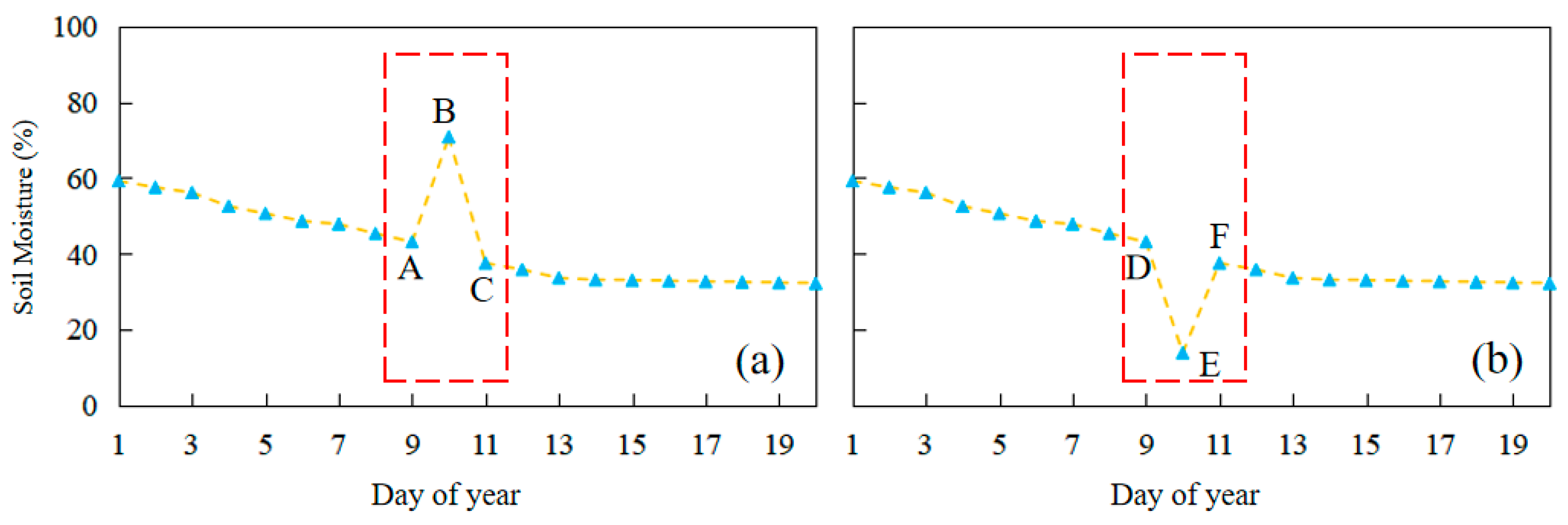
4.1. Extraction of Soil Moisture Increased Stage

Before extracting the soil moisture increased stage, two constraints are defined to constrain the soil moisture increased stage. First of all, in the soil moisture increased stage, soil moisture is greater than at a previous time. Second, soil moisture increases rapidly after an abundant water supplementation event, then smoothly recedes through evapotranspiration and drainage [44]. Extensive precipitation and irrigation can be considered an abundant water supplement event.
In addition, two types of abnormal soil moisture must be removed (Figure 4). As Figure 4a shows, soil moisture at time B presents a suddenly increase. Although soil moisture at time C is less than that at time B, soil moisture keeps increasing during the subsequent period of flow (i.e., C > A), so that soil moisture at times A, B, and C is assigned to the same soil moisture increased stage.
This section may be divided by subheadings. It should provide a concise and precise description of the experimental results, their interpretation, as well as the experimental conclusions that can be drawn.
The other type of abnormal soil moisture is shown in Figure 4b, with soil moisture at time E less than at time D but that at time F greater than at times E and D. In such a case, soil moisture at times A, B, and C is assigned to the same soil moisture increased stage. According to the constraints mentioned above, the soil moisture shown in Figure 4a or Figure 4b would not be classed as two independent soil moisture increased stages.
Abnormal soil moisture must also be removed during the soil moisture decreased stage (Figure 5). As Figure 5a shows, soil moisture at time B increases suddenly. Although soil moisture at time B is greater than at time A, soil moisture continues decreasing during the subsequent period of flow (C > B and C < A). Because the aforementioned conditions do not fit slow drying of soil after sufficient water input, soil moisture at times A, B, and C is classed as a single soil moisture decreased stage. In Figure 5b, soil moisture at time F is greater than at time E but less than at time D and continues decreasing during the subsequent period of flow. Accordingly, soil moisture in the AB and EF stages shown in Figure 5a,b is not classed as a soil moisture increased stage.
Figure 6 shows a flowchart for extracting the soil moisture increased stage using the following method:
Step 1: Add the first soil moisture at the start time, and flag it as O. Then, add the next adjacent soil moisture, and flag it as A. If A is less than O, A is reflagged as O, and then, the next adjacent soil moisture A is added. Otherwise, if A is greater than O, the next step will be continued. If the adjacent soil moisture is more than 7 days (about half the irrigation period in study area), this extracted process is ended, and a new extracted process is started.
Step 2: Add the next adjacent soil moisture, and flag it as B. If B is greater than A, B is reflagged as A and repeat Step 2. Otherwise, if B is less than A, continue to the next step.
Step 3: Add the next adjacent soil moisture, and flag it as C. If C is greater than A, C is re-flagged as A; return to Step 2. Using this progress, abnormal soil moisture such as that shown in Figure 4b can be eliminated. Otherwise, if C is less than A, the process compares B with C. If C is greater than B, B is re-flagged as A; return to Step 2. Step 3 can eliminate abnormal soil moisture, as shown in Figure 4b.
The first point in the soil moisture increased stage is the start time, and the last is the end time. The total precipitation during the soil moisture increased stage can also be calculated.

4.2. Construction of Fuzzy Membership Functions with which to Formulate the Relationship between Irrigation Necessity and Environmental Factors

A fuzzy membership function is used to describe the gradual transition between irrigation necessity and environment factors. Many expressions are used in fuzzy membership functions, such as the trigonometric-function and Gaussian-like function [45]. In this study, a general Gaussian-like function, which allows users to control the shape of the curve more easily, is adopted to describe the relationship between irrigation necessity and environmental factors (Equation (2)):
f i j k , v = e [ ( x 0 x i j k , v ) / w ] 2 ln ( c )
where f i j k , v is the irrigation necessity at point (i, j) and time k based on environmental factor v (e.g., precipitation and soil water), x i j k , v is the typical value of environmental variable v when the irrigation necessity is 1.0, and w is the difference between x 0 and the value of environmental factor at which the necessity value is 0.5 (c value).

(1) Fuzzy membership function for irrigation necessity with respect to soil moisture

In agricultural production, when relative soil moisture falls below 30%, drought ensues. If farmland cannot be irrigated during a drought, loss or even failure of the harvest can result. Accordingly, irrigation is necessary in such a situation. Conversely, when relative soil moisture exceeds 60%, no risk of drought is identified. Accordingly, the fuzzy membership value for irrigation necessity with respect to soil moisture can be set to 1 when relative soil moisture is below 30% but to 0 when relative soil moisture exceeds 60%.
Next, the value of soil moisture must be determined where the fuzzy membership value is 0.5. To this end, this study analyzes the in situ soil moisture before 60 instances of irrigation. The result shows that 30 instances of irrigation have a soil moisture below 48% relative soil moisture, or half of the 60 instances of irrigation. The fuzzy membership value for irrigation necessity with respect to soil moisture is, thus, 0.5 when the relative soil moisture is 48%.
Finally, the fuzzy membership function for irrigation necessity with respect to soil moisture can be described as follows:
f i j k , R s m = 1 ,   R s m < 0.3 , f i j k , R s m = e [ 0.3 x i j k , R s m 0.18 ] 2 ln ( 0.5 ) ,   0.3 R s m 0.6 , f i j k , R s m = 0 ,   R s m > 0.6
where f i j k , R s m is the irrigation necessity at point (i, j) and time k based on the relative soil moisture and Rsm is the relative soil moisture before the increase in soil moisture. The other parameters have the same meanings previously given.

(2) Fuzzy membership function for irrigation necessity with respect to precipitation

Because increases in soil moisture can be attributed to irrigation when no precipitation occurs, the fuzzy membership value for irrigation necessity with respect to precipitation is 1 when precipitation is 0 mm. In addition, based on daily average evapotranspiration (5–7 mm) and water efficiency of crops (52–66%), Chen et al. [18] used a threshold of 7.6 mm precipitation to distinguish effective and invalid precipitation. In this study, precipitation greater than 7.6 mm is considered effective precipitation and precipitation less than 7.6 mm invalid precipitation, with the fuzzy membership value with respect to precipitation considered to be 0.5 when precipitation is 7.6 mm.
The fuzzy membership function for irrigation necessity with respect to precipitation can, thus, be described as:
f i j k , P = e [   x i j k , P 7.6 ] 2 ln ( 0.5 ) ,       0 < P
where f i j k , P is irrigation necessity at point (i, j) and time k based on precipitation and P is the precipitation during the soil moisture increased stage. The other parameters have the same meanings previously given.

(3) Fuzzy membership function for irrigation necessity with respect to other factors

Crop phenology is an important factor in irrigation. For example, crops need more water during the filling stage than during other phenology stages. In some areas that suffer from water shortage, irrigation usually happens only during the filling stage, with farmers refraining from irrigating crops in other phenology stages to save water. Moreover, differences between regional economies will affect local investment in irrigation facilities, with irrigation occurring more frequently in areas that have greater investment in irrigation facilities. However, formulating fuzzy membership functions for irrigation necessity with respect to all environment factors can be very challenging, owing to a lack of data. In this study, fuzzy membership functions for irrigation necessity with respect to environment factors, such as crop phenology and regional economy, are assigned a constant value of 1.

4.3. Relevant Degree between Increased Soil Moisture and Irrigation

According to the operation rules of fuzzy sets, a model is established with which to infer the relevant degree between increased soil moisture and irrigation (Equation (5)):
M i , j , k   ( R s m k , P k ) = min ( f i j k , R s m , f i j k , P k ) = f i j k , R s m f i j k , P k
where ( i ,   j ) is the location of the satellite soil moisture pixel, k is the number of soil moisture increased stages, R s m is the relative soil moisture before increases in soil moisture, and P k is the precipitation during the soil moisture increase period. In addition, f i j k , R s m is the fuzzy membership function for irrigation necessity with respect to soil moisture, f i j k , P k is the fuzzy membership function with respect to precipitation, and M i , j , k   (   R s m k , P k ) is the relevant degree between increased soil moisture and irrigation for k soil moisture increased stages.
A minimum operator is used to calculate the relevant degree between increased soil moisture and irrigation, based on the principle of the limiting factor, whereby a process is affected by several different factors and its maximum rate is limited by its lowest factor, the limiting factor. Because irrigation is affected by several environmental factors, the membership degree of each must be synthesized. In reality, farmers will irrigate as little as possible to cut the costs of agricultural production, irrigating only when all environmental factors indicate its necessity. The principle of the limiting factor can be adopted to synthesize the membership degree of all environmental factors.
The relevant degree between each increase in soil moisture and irrigation can be calculated using the method already described and ranges from 0 to 1. A threshold is then adopted to defuzzify the relevant degree between increased soil moisture and irrigation. A discrete value (0 or 1) can be obtained to describe the relationship between increased soil moisture and irrigation, with 1 signifying irrigation as a cause and 0 signifying no attribution to irrigation.

4.4. Method of Validating Extracted Irrigation Signals

The extracted irrigation signals for 2016 and 2017 in Hebi City (two pixels in the study area) were validated due to lack of observed irrigation data. The irrigation period is confirmed using daily in situ soil moisture and precipitation data, after which the extracted irrigation signals are validated by the confirmed irrigation period, using the following method:
Step 1: Confirm irrigation using in situ soil moisture and precipitation data. According to surveys of the study area, a single irrigation cycle (from first day to last) usually lasts about 15 days. Thus, the irrigation period is limited to 15 days and increases in in situ soil moisture in the absence of precipitation regarded as signs of irrigation. In situ soil moisture is then analyzed at other sites, with in situ soil moisture sites bearing signs of irrigation counted for one irrigation period. The statistics are summarized in the following four levels: (1) more than one in situ soil moisture site with signs of irrigation, (2) more than two in situ soil moisture sites with signs of irrigation, (3) more than three in situ soil moisture sites with signs of irrigation, and (4) more than four in situ soil moisture sites with signs of irrigation. Using these divisions, the more in situ soil moisture sites with signs of irrigation during a given irrigation period, the higher the certainty that irrigation occurred in the corresponding pixel.
Step 2: Validate the extracted irrigation signal using the irrigation period confirmed in Step 1. If the extracted irrigation signal is in the irrigation period, it is deemed to be correct, otherwise not.

5. Results

5.1. Validation of the Extracted Irrigation Signals

The extracted irrigation signals of 2016 and 2017 in Hebi City (two pixels in the study area) are validated due to lack of observed irrigation data at the pixel scale. Table 3 shows the number of correctly extracted irrigation signals which are compared with observed irrigation data. As shown in Table 3, 22 irrigation signals are extracted within a defuzzification threshold of 0.6, 18 irrigation signals are extracted within a defuzzification threshold of 0.7, 10 irrigation signals are extracted within a defuzzification threshold of 0.8, and 10 irrigation signals are extracted within a defuzzification threshold of 0.9. As shown in line 1 of Table 3, each of the 31 observed irrigation periods has more than one in situ soil moisture site with signs of irrigation. At a defuzzification threshold of 0.6, 18 of the 31 periods have at least one irrigation signal in each. At a threshold of 0.7, that figure is 16; at thresholds of 0.8 and 0.9, it is 10.
As line 4 of Table 3 shows, each of four observed irrigation periods has more than four in situ soil moisture sites with signs of irrigation. At defuzzification thresholds of 0.6 and 0.7, all four observed irrigation periods have at least one irrigation signal in each of them; at thresholds of 0.8 and 0.9, that figure is three. As the row data show, recognized accuracy decreases with increases in the defuzzification threshold, showing that the method proposed in this study cannot recognize small-scale irrigation within a large defuzzification threshold. The column data in Table 3 show that with high certainty about the observed irrigation period, almost all observed irrigation periods can be recognized. Finally, the defuzzification threshold of 0.6 is chosen to defuzzify the relevant degree between increased soil moisture and irrigation.
Irrigation experienced in the study area is also used to qualitatively verify the extracted irrigation signal. Table 4 shows the start and end times of extracted irrigation signals, showing that most irrigation occurred from late February to early May (Days 30–100), with 12 irrigation signals extracted for this period. Another period of intensive irrigation occurred from late October to early December, with seven irrigation signals extracted for this period.
In Table 4, the first period (Days 30–100) of intensive irrigation signals contains several key growth periods of winter wheat, including the returning green stage (mid-February to early to mid-March), elongation stage (April), and grain filling stage (early May). Based on the irrigation experienced in the study area, winter wheat usually needs irrigating in these stages. The second period of intensive irrigation signals occurred from the sowing stage to the wintering stage (late October to early November), when wheat sowing also requires irrigation. In normal years, winter wheat requires irrigation during the tilling stage (mid-November) and wintering stage (late November to early December).

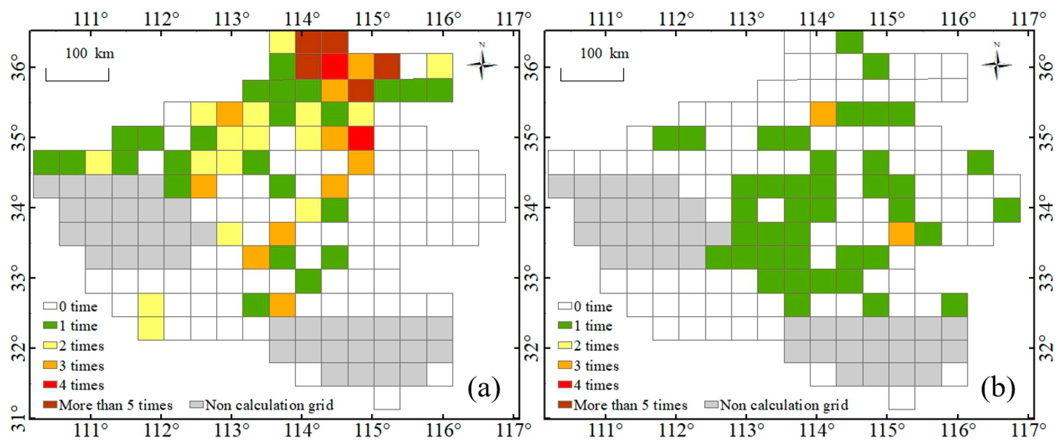
5.2. Irrigation Frequency in Henan Province

When using the proposed method to extract irrigation signals in Henan Province, for convenient presentation of the extracted signals, one irrigation signal in satellite-based soil moisture data is regarded as a single instance of irrigation at the pixel scale, with the extracted signals shown as irrigation frequency. It should be noted that the proposed method is applied in dry cultivated areas but neglected where paddy fields account for more than 10% of the total area or dry land for less than 10% of the total area.
Based on the extracted irrigation signals, irrigation frequency maps for 2016 and 2017 are obtained (Figure 7). The gray pixels in Figure 7 are paddy field accounting for more than 10% of pixels or dry land accounting for less than 10% of pixels. The spatial pattern of the irrigation frequency maps shows a decreasing trend from north to south.
Figure 8 shows irrigation frequency maps in the winter crops’ growth season (Figure 8a) and summer crops’ growth season (Figure 8b). From Figure 8, it can be found that irrigation is more frequent in winter crops’ growth season than in summer crops’ growth season. This phenomenon can be ascribed to the uneven distribution of precipitation in this region. Henan Province is located in the North China Plain and is affected by the Asian monsoon climate. Summer is hot and rainy, accounting for 50–80% of the year’s precipitation, but late autumn to late spring of the second year accounts for only about 30% of the year’s precipitation. Winter wheat is the main crop in Henan Province, with more than three to five instances of irrigation usually needed during winter wheat’s growth period. Figure 8b shows an irrigation frequency map of summer crops’ growth season, with irrigation occurring mainly in the middle of the study area during the sowing stage (late May to early June). The dryness of the soil during this period calls for irrigation to keep the soil moist and ensure seeds’ germination.

5.3. Spatial Analysis of the Irrigation Frequency Map

Figure 9 shows an irrigation area map of Henan Province [46], with irrigated area showing a decreasing trend from north to south. The maximum amount of irrigated area can reach 90%, with the average irrigation area in northern Henan Province exceeding 85%. The irrigation frequency depicted in Figure 9 is also high in northern Henan Province, where the maximum value can exceed six instances. The spatial pattern of irrigation frequency, thus, accords well with the irrigation area map.
Figure 10 shows the annual precipitation (a,b), annual potential evapotranspiration (c,d), and differences in precipitation and potential evapotranspiration (e,f) for 2016 and 2017 in Henan Province. The minimum precipitation occurred in north Henan Province and the maximum in south Henan Province. The 2016 and 2017 annual precipitation maps both show a decreasing trend from north to south, whereas the potential evapotranspiration maps show an increasing trend from north to south. As Figure 10e,f show, precipitation could be 400 mm less than the potential evapotranspiration in the north of study area.
As Figure 10 shows, the spatial pattern of precipitation varies inversely with the irrigation frequency, whereas the spatial pattern of potential evapotranspiration is consistent with that of irrigation frequency—a phenomenon that appeals to the common sense of irrigation, which is not needed in areas with much precipitation and little evapotranspiration. However, in areas where precipitation is sparse and evapotranspiration is significant, more irrigation is needed.

6. Discussion

The proposed method in this study is used to extract irrigation signals from the in SMAP L3 Passive Soil Moisture Product. The extracted irrigation signals of two grids of SMAP data (Hebi City in Henan Province) are validated using daily in situ soil moisture and precipitation, revealing that most irrigation signals are extracted correctly. By grading the fuzzy membership degree, irrigation frequency maps of the 2016–2017 winter crop growth season and the 2017 summer crop growth season are obtained. Compared with precipitation maps and potential evapotranspiration maps, irrigation frequency maps showed a spatial pattern opposite to that of precipitation maps and a spatial pattern similar to that of potential evapotranspiration maps, indicating that the spatial pattern of irrigation frequency maps are reasonable in space.
However, it should be noted that this study only represents a meaningful attempt to extract irrigation signals using a coarse-resolution satellite-based soil moisture product. The satellite-based soil moisture data adapted in this study are from the SMAP L3 Passive Soil Moisture Product (36 km × 36 km). The irrigation observation data used in the qualitative assessments are rendered less convincing by the coarse resolution of SMAP soil moisture data. As a result, quantitative validation of extracted irrigation signals remains challenging. In addition, because small-scale irrigation cannot be captured by a coarse-resolution satellite-based soil moisture product, a high-resolution satellite-based soil moisture product is needed to extract irrigation signals.
In recent research, Lawston et al. [28] and Hao et al. [32] verified that the SMAP enhanced L3 radiometer global daily 9 km EASE-grid soil moisture can capture irrigation signals. These studies represent a meaningful attempt to extract irrigation signals using a high-resolution satellite-based soil moisture product, and as further high-resolution satellite-based soil moisture products (e.g., Sentinel-1 soil moisture retrievals, SMAP/Sentinel-1 soil moisture product) become available, the method proposed in this study can be further validated using high-resolution satellite-based soil. Moreover, previous study has proven that some vegetation indexes increase sharply after precipitation or irrigation during the vegetation growth stage [18]. However, Chen et al. [18] only used one environmental factor of rainfall to identify irrigation signals. The method that takes into account of multiple environmental factors in irrigation could also be a new attempt of extraction of irrigation signals by using optical remote sensing data.

7. Conclusions

Previous studies usually used effective rainfall threshold to distinguish irrigation signals and nonirrigation signals. In those studies, the increased stages in satellite-based soil moisture that have effective rainfall were identified as the irrigation signal, while the increased stages in satellite-based soil moisture that have no effective rainfall were identified as the nonirrigation signal. The method is easy to implement but cannot express the relationship between irrigation and environmental factors: because only one environmental factor of rainfall is used to identify irrigation signals, other environmental factors, such as initial soil moisture conditions, cannot be taken into consideration.
Accordingly, this study developed an irrigation signal extraction method that takes into account multiple environmental factors affecting irrigation. Firstly, the fuzzy membership functions of irrigation relating to multiple environmental factors (e.g., precipitation and soil water) are constructed. Then, a model is built based on the fuzzy membership functions by using operation rules of fuzzy sets, which is used to infer the relevant degree of irrigation to nonirrigation. Finally, irrigation signals in satellite-based soil moisture data are recognized according to the relevant degree. Taking Henan Province in the North China Plain as the study area, the proposed method is used to extract irrigation signals from the SMAP Level 3 Passive Soil Moisture Product, and the extracted irrigation signals from two SMAP grids are validated using daily in situ soil moisture and precipitation data. The results show that most of the irrigation signals are identified correctly. By grading the membership degree of the extracted irrigation signals, irrigation frequency maps of the 2016–2017 winter crop growth season and the 2017 summer crop growth season are obtained for Henan Province. Compared to the irrigation frequency maps with data on the annual precipitation and the annual potential evapotranspiration, the irrigation frequency maps show a spatial pattern opposite to that of the annual precipitation and a spatial pattern similar to that of annual potential evapotranspiration, indicating that the spatial pattern of irrigation frequency maps are reasonable.

Author Contributions

Conceptualization, L.Z. and A.-X.Z.; methodology, L.Z.; software, L.Z.; validation, L.Z.; formal analysis, L.Z.; investigation, L.Z.; resources, L.Z.; data curation, L.Z.; writing—original draft preparation, L.Z. and A.-X.Z.; writing—review and editing, L.Z. and A.-X.Z.; visualization, L.Z.; supervision, A.-X.Z.; project administration, L.Z.; funding acquisition, L.Z. All authors have read and agreed to the published version of the manuscript.

Funding

This research was funded by the Postdoctoral Research Funding Program of Jiangsu Province (Grant No. 2020Z223), the Project of Green Yang and Golden Phoenix, and the National Natural Science Foundation of China (Grant No. 41771478).

Institutional Review Board Statement

Not applicable.

Informed Consent Statement

Not applicable.

Data Availability Statement

Not applicable.

Conflicts of Interest

The authors declare no conflict of interest.

References

  1. Siebert, S.; Doll, P.; Hoogeveen, J.; Faures, J.M.; Frenken, K.; Feick, S. Development and validation of the global map of irrigation areas. Hydrol. Earth Syst. Sci. 2005, 9, 535–547. [Google Scholar] [CrossRef]
  2. Godfray, H.C.J.; Beddington, J.R.; Crute, I.R.; Haddad, L.; Lawrence, D.; Muir, J.F.; Pretty, J.; Robinson, S.; Thomas, S.M.; Toulmin, C. Food Security: The Challenge of Feeding 9 Billion People. Science 2010, 327, 812–818. [Google Scholar] [CrossRef] [PubMed] [Green Version]
  3. Troy, T.J.; Kipgen, C.; Pal, I. The impact of climate extremes and irrigation on US crop yields. Environ. Res. Lett. 2015, 10, 054013. [Google Scholar] [CrossRef] [Green Version]
  4. Zhang, C.; Liu, J.G.; Shang, J.L.; Cai, H.J. Capability of crop water content for revealing variability of winter wheat grain yield and soil moisture under limited irrigation. Sci. Total Environ. 2018, 631–632, 677–687. [Google Scholar] [CrossRef]
  5. Lobell, D.B.; Bonfils, C. The effect of irrigation on regional temperatures: A spatial and temporal analysis of trends in California, 1934–2002. J. Clim. 2008, 21, 2063–2071. [Google Scholar] [CrossRef]
  6. Leng, G.Y.; Huang, M.Y.; Tang, Q.H.; Leung, L.R. A modeling study of irrigation effects on global surface water and groundwater resources under a changing climate. J. Adv. Model. Earth Syst. 2015, 7, 1285–1304. [Google Scholar] [CrossRef]
  7. Tang, Q.; Rosenberg, E.A.; Lettenmaier, D.P. Use of satellite data to assess the impacts of irrigation withdrawals on Upper Klamath Lake, Oregon. Hydrol. Earth Syst. Sci. 2009, 13, 617–627. [Google Scholar] [CrossRef] [Green Version]
  8. Nazemi, A.; Wheater, H.S. On inclusion of water resource management in Earth system models—Part 2: Representation of water supply and allocation and opportunities for improved modeling. Hydrol. Earth Syst. Sci. 2015, 19, 63–90. [Google Scholar] [CrossRef] [Green Version]
  9. Nazemi, A.; Wheater, H.S. On inclusion of water resource management in Earth system models—Part 1: Problem definition and representation of water demand. Hydrol. Earth Syst. Sci. 2015, 19, 33–61. [Google Scholar] [CrossRef] [Green Version]
  10. Elliott, J.; Deryng, D.; Mueller, C.; Frieler, K.; Konzmann, M.; Gerten, D.; Glotter, M.; Floerke, M.; Wada, Y.; Best, N.; et al. Constraints and potentials of future irrigation water availability on agricultural production under climate change. Proc. Natl. Acad. Sci. USA 2014, 111, 3239–3244. [Google Scholar] [CrossRef] [PubMed] [Green Version]
  11. Kang, S.; Eltahir, E.A.B. North China Plain threatened by deadly heatwaves due to climate change and irrigation. Nat. Commun. 2018, 9, 2894. [Google Scholar] [CrossRef] [Green Version]
  12. Portmann, F.T.; Siebert, S.; Döll, P. MIRCA2000—Global monthly irrigated and rainfed crop areas around the year 2000: A new high-resolution data set for agricultural and hydrological modeling. Glob. Biogeochem. Cycles 2010, 24, GB1011. [Google Scholar] [CrossRef]
  13. Ozdogan, M. Exploring the potential contribution of irrigation to global agricultural primary productivity. Glob. Biogeochem. Cycles 2011, 25, B3016. [Google Scholar] [CrossRef]
  14. Foster, T.; Mieno, T.; Brozovi, T. Satellite-based Monitoring of Irrigation Water Use: Assessing Measurement Errors and Their Implications for Agricultural Water Management Policy. Water Resour. Res. 2020, 56, e2020WR028378. [Google Scholar] [CrossRef]
  15. Ozdogan, M.; Gutman, G. A new methodology to map irrigated areas using multi-temporal MODIS and ancillary data: An application example in the continental US. Remote Sens. Environ. 2008, 112, 3520–3537. [Google Scholar] [CrossRef] [Green Version]
  16. Thenkabail, P.S.; Biradar, C.M.; Noojipady, P.; Dheeravath, V.; Li, Y.J.; Velpuri, M.; Gumma, M.; Gangalakunta, O.R.P.; Turral, H.; Cai, X.L.; et al. Global irrigated area map (GIAM), derived from remote sensing, for the end of the last millennium. Int. J. Remote Sens. 2009, 30, 3679–3733. [Google Scholar] [CrossRef]
  17. Pervez, M.S.; Budde, M.; Rowland, J. Mapping irrigated areas in Afghanistan over the past decade using MODIS NDVI. Remote Sens. Environ. 2014, 149, 155–165. [Google Scholar] [CrossRef] [Green Version]
  18. Chen, Y.; Lu, D.; Luo, L.; Pokhrel, Y.; Deb, K.; Huang, J.; Ran, Y. Detecting irrigation extent, frequency, and timing in a heterogeneous arid agricultural region using MODIS time series, Landsat imagery, and ancillary data. Remote Sens. Environ. 2017. [Google Scholar] [CrossRef]
  19. Xiao, X.; Boles, S.; Liu, J.; Zhuang, D.; Frolking, S.; Li, C.; Salas, W.; Iii, B.M. Mapping paddy rice agriculture in southern China using multi-temporal MODIS images. Remote Sens. Environ. 2005, 95, 480–492. [Google Scholar] [CrossRef]
  20. Pena-Arancibia, J.L.; McVicar, T.R.; Paydar, Z.; Li, L.T.; Guerschman, J.P.; Donohue, R.J.; Dutta, D.; Podger, G.M.; van Dijk, A.; Chiew, F.H.S. Dynamic identification of summer cropping irrigated areas in a large basin experiencing extreme climatic variability. Remote Sens. Environ. 2014, 154, 139–152. [Google Scholar] [CrossRef]
  21. Kolassa, J.; Gentine, P.; Prigent, C.; Aires, F.; Alemohammad, S.H. Soil moisture retrieval from AMSR-E and ASCAT microwave observation synergy. Part 2: Product evaluation. Remote Sens. Environ. 2017, 195, 202–217. [Google Scholar] [CrossRef]
  22. Kerr, Y.H.; Al-Yaari, A.; Rodriguez-Fernandez, N.; Parrens, M.; Molero, B.; Leroux, D.; Bircher, S.; Mahmoodi, A.; Mialon, A.; Richaume, P.; et al. Overview of SMOS performance in terms of global soil moisture monitoring after six years in operation. Remote Sens. Environ. 2016, 180, 40–63. [Google Scholar] [CrossRef]
  23. Pan, M.; Cai, X.T.; Chaney, N.W.; Entekhabi, D.; Wood, E.F. An initial assessment of SMAP soil moisture retrievals using high-resolution model simulations and in situ observations. Geophys. Res. Lett. 2016, 43, 9662–9668. [Google Scholar] [CrossRef] [Green Version]
  24. An, R.; Zhang, L.; Wang, Z.; Quaye-Ballard, J.A.; You, J.J.; Shen, X.J.; Gao, W.; Huang, L.J.; Zhao, Y.H.; Ke, Z.Y. Validation of the ESA CCI soil moisture product in China. Int. J. Appl. Earth Obs. Geoinf. 2016, 48, 28–36. [Google Scholar] [CrossRef]
  25. Kumar, S.V.; Peters-Lidard, C.D.; Santanello, J.A.; Reichle, R.H.; Draper, C.S.; Koster, R.D.; Nearing, G.; Jasinski, M.F. Evaluating the utility of satellite soil moisture retrievals over irrigated areas and the ability of land data assimilation methods to correct for unmodeled processes. Hydrol. Earth Syst. Sci. 2015, 19, 4463–4478. [Google Scholar] [CrossRef] [Green Version]
  26. Qiu, J.X.; Gao, Q.Z.; Wang, S.; Su, Z.R. Comparison of temporal trends from multiple soil moisture data sets and precipitation: The implication of irrigation on regional soil moisture trend. Int. J. Appl. Earth Obs. Geoinf. 2016, 48, 17–27. [Google Scholar] [CrossRef]
  27. Singh, D.; Gupta, P.K.; Pradhan, R.; Dubey, A.K.; Singh, R.P. Discerning shifting irrigation practices from passive microwave radiometry over Punjab and Haryana. J. Water Clim. Chang. 2017, 8, 303–319. [Google Scholar] [CrossRef] [Green Version]
  28. Lawston, P.M.; Santanello, J.A.; Kumar, S.V. Irrigation Signals Detected From SMAP Soil Moisture Retrievals. Geophys. Res. Lett. 2017, 44, 11860–11867. [Google Scholar] [CrossRef] [Green Version]
  29. Brocca, L.; Tarpanelli, A.; Filippucci, P.; Dorigo, W.; Zaussinger, F.; Gruber, A.; Fernandez-Prieto, D. How much water is used for irrigation? A new approach exploiting coarse resolution satellite soil moisture products. Int. J. Appl. Earth Obs. Geoinf. 2018, 73, 752–766. [Google Scholar] [CrossRef]
  30. Jalilvand, E.; Tajrishy, M.; Hashemi, S.; Brocca, L. Quantification of irrigation water using remote sensing of soil moisture in a semi-arid region. Remote Sens. Environ. 2019, 231, 111226. [Google Scholar] [CrossRef]
  31. Zaussinger, F.; Dorigo, W.; Gruber, A.; Tarpanelli, A.; Filippucci, P.; Brocca, L. Estimating irrigation water use over the contiguous United States by combining satellite and reanalysis soil moisture data. Hydrol. Earth Syst. Sci. 2019, 23, 897–923. [Google Scholar] [CrossRef] [Green Version]
  32. Al-Yaari, A.; Ducharne, A.; Cheruy, F.; Crow, W.T.; Wigneron, J.P. Satellite-based soil moisture provides missing link between summertime precipitation and surface temperature biases in CMIP5 simulations over conterminous United States. Sci. Rep. 2019, 9, 1657. [Google Scholar] [CrossRef] [Green Version]
  33. Hao, Z.; Zhao, H.L.; Zhang, C.; Wang, H.; Jiang, Y.Z. Detecting Winter Wheat Irrigation Signals Using SMAP Gridded Soil Moisture Data. Remote Sens. 2019, 11, 2390. [Google Scholar] [CrossRef] [Green Version]
  34. Zadeh, L.A. Fuzzy sets. Fuzzy Sets, Fuzzy Logic, & Fuzzy Systems; World Scientific Publishing Co., Inc.: New York, NY, USA, 1996; pp. 394–432. [Google Scholar]
  35. Zhu, A. A personal construct-based knowledge acquisition process for natural resource mapping. Int. J. Geogr. Inf. Syst. 1999, 13, 119–141. [Google Scholar] [CrossRef]
  36. Zhu, A.X.; Hudson, B.; Burt, J.; Lubich, K.; Simonson, D. Soil mapping using GIS, expert knowledge, and fuzzy logic. Soil Sci. Soc. Am. J. 2001, 65, 1463–1472. [Google Scholar] [CrossRef] [Green Version]
  37. Zhu, L.; Liu, J.; Zhu, A.X.; Sheng, M.; Duan, Z. Spatial Distribution of Diurnal Rainfall Variation in Summer over China. J. Hydrometeorol. 2018, 19, 667–678. [Google Scholar] [CrossRef]
  38. Zhang, X.F.; Zhang, T.T.; Zhou, P.; Shao, Y.; Gao, S. Validation Analysis of SMAP and AMSR2 Soil Moisture Products over the United States Using Ground-Based Measurements. Remote Sens. 2017, 9, 104. [Google Scholar] [CrossRef] [Green Version]
  39. Cui, H.Z.; Jiang, L.M.; Du, J.Y.; Zhao, S.J.; Wang, G.X.; Lu, Z.; Wang, J. Evaluation and analysis of AMSR-2, SMOS, and SMAP soil moisture products in the Genhe area of China. J. Geophys. Res. Atmos. 2017, 122, 8650–8666. [Google Scholar] [CrossRef]
  40. Kim, H.; Parinussa, R.; Konings, A.G.; Wagner, W.; Cosh, M.H.; Lakshmi, V.; Zohaib, M.; Choi, M. Global-scale assessment and combination of SMAP with ASCAT (active) and AMSR2 (passive) soil moisture products. Remote Sens. Environ. 2018, 204, 260–275. [Google Scholar] [CrossRef]
  41. Zhu, L.M.; Liu, J.Z.; Zhu, A.X.; Duan, Z. Spatial evaluation of L-band satellite-based soil moisture products in the upper Huai River basin of China. Eur. J. Remote Sens. 2019, 52, 194–205. [Google Scholar] [CrossRef] [Green Version]
  42. Colliander, A.; Jackson, T.J.; Bindlish, R.; Chan, S.; Das, N.; Kim, S.B.; Cosh, M.H.; Dunbar, R.S.; Dang, L.; Pashaian, L.; et al. Validation of SMAP surface soil moisture products with core validation sites. Remote Sens. Environ. 2017, 191, 215–231. [Google Scholar] [CrossRef]
  43. Shen, Y.; Zhao, P.; Pan, Y.; Yu, J.J. A high spatiotemporal gauge-satellite merged precipitation analysis over China. J. Geophys. Res. Atmos. 2014, 119, 3063–3075. [Google Scholar] [CrossRef]
  44. Brocca, L.; Ciabatta, L.; Massari, C.; Moramarco, T.; Hahn, S.; Hasenauer, S.; Kidd, R.; Dorigo, W.; Wagner, W.; Levizzani, V. Soil as a natural rain gauge: Estimating global rainfall from satellite soil moisture data. J. Geophys. Res. Atmos. 2014, 119, 5128–5141. [Google Scholar] [CrossRef]
  45. Zhu, A.; Lin, Y.; Li, B.L.; Qin, C.Z.; Tao, P.; Liu, B.Y.; Minasny, B.; Lark, M.; Behrens, T. Construction of membership functions for predictive soil mapping under fuzzy logic. Geoderma 2010, 155, 164–174. [Google Scholar] [CrossRef]
  46. ORNL DAAC. Spatial Data Access Tool (SDAT); ORNL DAAC: Oak Ridge, TN, USA, 2017. [Google Scholar] [CrossRef]
Figure 1. (a) Time series SMAP soil moisture and precipitation at one SMAP pixel. (b) In situ soil moisture at seven sites in the SMAP pixel.
Remotesensing 13 02142 g001
Figure 2. (a) Land use and land cover of study area, with locations of SMAP grids. (b) Locations of the 16 in situ soil moisture sites in Hebi City. (c) Environment of each in situ soil moisture site.
Remotesensing 13 02142 g002
Figure 3. In situ soil moisture, precipitation, and observed irrigation records at the 53992 station for 2017.
Remotesensing 13 02142 g003
Figure 4. Schematic of abnormal soil moisture in the soil moisture increased stage. (a) soil moisture at time A less than at time B and C, but that at time B greater than at times C. (b) soil moisture at time E less than at time D but that at time F greater than at times E and D.
Remotesensing 13 02142 g004
Figure 5. Schematic of abnormal soil moisture in the soil moisture decreased stage. (a) soil moisture at time A less than at time B, but that at time B greater than at times C. (b) soil moisture at time D less than at time F but that at time D greater than at times E.
Remotesensing 13 02142 g005
Figure 6. Flowchart of extracting soil moisture increased period.
Remotesensing 13 02142 g006
Figure 7. Irrigation frequency maps at a threshold of 0.6 for (a) 2016 and (b) 2017.
Remotesensing 13 02142 g007
Figure 8. Irrigation frequency maps during the growth seasons for (a) winter crops and (b) summer crops.
Remotesensing 13 02142 g008
Figure 9. Distribution map of irrigated extent and irrigation area in Henan Province (ORNL DAAC. 2017).
Remotesensing 13 02142 g009
Figure 10. (a,b) show the annual precipitation for 2016 and 2017. (c,d) show the annual potential evapotranspiration for 2016 and 2017, calculated using the Penman–Monteith formula (Allen, 1998). (e,f) show the difference between the annual precipitation and the annual potential evapotranspiration.
Remotesensing 13 02142 g010
Table 1. Key papers for detection/extraction of irrigation signals from satellite-based soil moisture.
StudySoil Moisture DataLocationDetection/ExtractionMethod
1. Kumar et al. (2015)AMSR-E
AMSR2
SMOS
ASCAT
Simulated soil moisture
Over the continental USDetectionCompare satellite soil moisture to the model simulated soil moisture that does not simulate irrigation.
2. Qiu et al. (2016)ESA CCI Soil Moisture
In situ soil moisture
Over the mainland of ChinaDetectionCompare satellite soil moisture to in situ soil moisture.
3. Singh et al. (2017)AMSR-EPunjab and Haryana states in IndiaDetectionCompare satellite soil moisture in irrigated area to that in rain-fed area.
4. Lawston et al. (2015)SMAP_EThree valleys in the USDetectionCompare satellite soil moisture in irrigated area to that in non-irrigated area.
5. Brocca et al. (2018)SMAP_P
SMOS
ASCAT
AMSR-2
Nine pilot sites in Europe, USA, Australia and AfricaDetectionCalculate input water by using SM2RAIN algorithm and satellite soil moisture; compare the input water to the observed precipitation data.
6. Jalilvand et al. (2019)AMSR2Miandoab plain in IranDetectionSame method as Brocca et al. (2018).
7. Zaussinger et al. (2019)SMAP_P
AMSR2
ASCAT
Reanalysis soil moisture
Over the continental USDetectionSame method as Brocca et al. (2018).
8. Al-Yaari et al. (2019)SMOS
ESA CCI Soil Moisture
Reanalysis soil moisture
Over the continental USDetection Analyze the link between spatial patterns of summertime satellite soil moisture, precipitation, and air temperature biases in 20 different CMIP5 simulations.
9. Hao et al. (2019)SMAP_EHebei Province in ChinaExtractionExtract out irrigation signals by setting precipitation threshold.
10. This studySMAP_PHenan Province in ChinaExtractionDevelop an irrigation signal extraction method that takes into account multiple environmental factors in irrigation.
Table 2. Locations and land use for the 16 in situ soil moisture sites.
NumberStation IDLongitudeLatitudeLand Use
153974114.18335.616Irrigated farmland
2O2063114.2335.565Irrigated farmland
3O2647114.17135.553Irrigated farmland
4O2913114.17435.736Irrigated farmland
5O2922114.10735.728Irrigated farmland
653990114.31535.715Irrigated farmland
753992114.57435.759Nonirrigated land
8O2067114.57235.766Irrigated farmland
9O2068114.32235.492Irrigated farmland
10O2069114.4735.667Irrigated farmland
11O2073114.29135.67Irrigated farmland
12O2850114.4235.58Irrigated farmland
13O2907114.60635.666Irrigated farmland
14O2908114.6635.74Irrigated farmland
15O2909114.44135.811Irrigated farmland
16O2910114.3535.61Nonirrigated land
Table 3. The observed irrigation signals are obtained using daily in situ soil moisture and precipitation. Within various defuzzification thresholds, different irrigation signals are correctly extracted. The thresholds refer to the relevant degree between increased soil moisture and irrigation.
Station (s)
#
Observed
##
Threshold 0.6 *Threshold 0.7 *Threshold
0.8 *
Threshold
0.9 *
13118161010
21611966
387766
444433
#: More than # station(s) monitored irrigation during a period. ##: Number of observed instances of irrigation. *: Number of extracted irrigation signals located in the observed irrigation period.
Table 4. Start and end times (day of year) of extracted irrigation signals in Hebi City at two pixels.
20162017
Pixel 1Pixel 2Pixel 1Pixel 2
58–6044–-45113–11817–22
95–10050–52132–13425–36
327–33082–84329–33239–41
90–92345–34865–68
95–100358–359225–228
223–226332–335
327–332345–348
Publisher’s Note: MDPI stays neutral with regard to jurisdictional claims in published maps and institutional affiliations.

