Abstract
Recent computer vision techniques based on convolutional neural networks (CNNs) are considered state-of-the-art tools in weed mapping. However, their performance has been shown to be sensitive to image quality degradation. Variation in lighting conditions adds another level of complexity to weed mapping. We focus on determining the influence of image quality and light consistency on the performance of CNNs in weed mapping by simulating the image formation pipeline. Faster Region-based CNN (R-CNN) and Mask R-CNN were used as CNN examples for object detection and instance segmentation, respectively, while semantic segmentation was represented by Deeplab-v3. The degradations simulated in this study included resolution reduction, overexposure, Gaussian blur, motion blur, and noise. The results showed that the CNN performance was most impacted by resolution, regardless of plant size. When the training and testing images had the same quality, Faster R-CNN and Mask R-CNN were moderately tolerant to low levels of overexposure, Gaussian blur, motion blur, and noise. Deeplab-v3, on the other hand, tolerated overexposure, motion blur, and noise at all tested levels. In most cases, quality inconsistency between the training and testing images reduced CNN performance. However, CNN models trained on low-quality images were more tolerant against quality inconsistency than those trained by high-quality images. Light inconsistency also reduced CNN performance. Increasing the diversity of lighting conditions in the training images may alleviate the performance reduction but does not provide the same benefit from the number increase of images with the same lighting condition. These results provide insights into the impact of image quality and light consistency on CNN performance. The quality threshold established in this study can be used to guide the selection of camera parameters in future weed mapping applications.
1. Introduction
Choosing the right camera parameters and lighting conditions is a critical consideration for researchers and engineers trying to obtain the best possible computer vision result in agricultural applications [1,2,3]. There are numerous camera choices on the market, each with many adjustable parameters. Furthermore, the surrounding environments, especially the lighting conditions, vary across different image collection events and times, severely complicating the decision-making process. Unfortunately, limited research has been conducted to provide insight into the vision system settings that are most suitable for weed mapping applications. Inappropriate selections may lead to unsatisfactory mapping results, and re-collecting images using new settings may be expensive and sometimes impossible.
Recent computer vision techniques based on convolutional neural networks (CNNs) are considered state-of-the-art tools in agriculture. Kamilaris and Prenafeta-Boldú [4] reported in a literature survey that CNNs were employed for object detection in 42% of the surveyed agriculture-related papers, and that they typically outperform traditional image processing techniques. Using YOLOv3, a popular CNN framework, Gao et al. [5] obtained average precisions of 76.1% and 89.7%, respectively, for the detection of hedge bindweed (Convolvulus sepium) and sugar beet, with a 6.48 ms inference time per image, illustrating the great potential of CNNs for weed mapping applications.
Despite the impressive accuracy and speed of CNNs, they have been shown to be sensitive to image degradation. Various types of image degradation, including Gaussian blur, motion blur, out-of-focus blur, reduced contrast, compression, fish-eye distortion, reduced resolution, salt-and-pepper noise, Gaussian noise, haziness, underwater effect, color distortion, and occlusion have been simulated by researchers to study their influence on CNN performance [6,7,8,9,10]. Although results showed varying degrees of impact on the performance of CNN, a major drawback in these studies was that all the image degradation simulations were performed on the images that were already processed by cameras or computers, which do not sufficiently represent real image degradations that occur in a camera [11]. Moreover, the reported degradation levels cannot be related to real camera parameters, which further limits their utility.
In addition to image quality, variation in illumination adds another level of complexity to weed mapping since it has enormous effects on the appearance of objects [12]. Variations in light direction result in shadows of different shape and position. Shifts in the light spectrum affect the pixel intensities of each color channel in an image [13]. Spotlights, such as the sun, tend to create highlights on objects, while area light sources such as light-emitting diode (LED) light panels tend to make objects appear flattened [14]. Peng et al. [15] simulated human face images under different illuminations and found that a face under non-uniformly distributed light has greatly reduced feature similarity to the same face under frontal light.
Standardizing computer vision systems may help address the issues associated with image degradation and light variation [16,17], but is difficult to achieve in weed mapping. Camera choices are often affected by the budget and commercial availability. This is especially true for drone-mounted cameras as they are often sold as an integrated component of a drone that is expensive to replace. Moreover, new camera models are launched by manufacturers at a fast rate and old models are typically terminated. Lighting condition is another factor that is difficult to control. Artificial lighting can be an option for proximal weed mapping, but is virtually impossible for remote mapping.
To our knowledge, no research has been done in the weed mapping domain to determine the influence of image quality and light consistency on CNN performance. Yet, a wide range of cameras have been used under different lighting conditions to collect various weed image datasets [18,19,20]. Because the plant species, resolution, image channel number and lighting conditions are all different in these datasets, comparison of CNN performance between these datasets is likely to result in ambiguous or misleading conclusions. In order to determine the minimum quality that should be met for image dataset collection to train CNNs in weed mapping tasks, a robust approach is to simulate the image formation pipeline for different image qualities [21].
In this research, we aim to gain insights into the influence of image quality and light consistency on the performance of CNNs for weed mapping by utilizing the image formation pipeline shown in Figure 1 (described further in Section 2). This pipeline is simulated with the introduction of various image alterations (quality degradations and enhancements) and light parameters to test their effect on CNN performance.
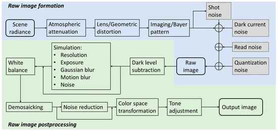
Figure 1.
Raw image formation and postprocessing pipeline. Redrawn from Tsin et al. [22], Liu et al. [23], and Sumner [24] based on the noise model proposed by Healey and Kondepudy [25].
2. Background
2.1. Formation of Raw Images
Digital images are formed from photons emitted by light sources and reflected from object surfaces. The photons are then diffracted through the camera lens and projected onto the detector array inside the camera. Each photon produces an electrical response at a specific site on the detector array, and the resulting signals are transformed electronically into a grid of pixel values. Pixel values thus convey the information of physical properties and conditions of the light sources and scenes.
The digital camera image formation pipeline can be grouped into a sequence of modules that describe the scene, optics, sensor, and processor [26]. For a given scene, the optical system of a camera first linearly converts scene radiance into irradiance on the detector array [27]. However, lens imperfections, defocus, and light diffraction limit the precision of scene reproduction on the camera sensor. These factors can cause image blur and can be collectively modeled as a convolution between the ideal sensor irradiance map and a point spread function (PSF) [28,29,30]. The irradiance map is commonly filtered by a Bayer filter to separate red, green and blue color bands [31]. As a result, a single pixel location is only able to record one color. The sensor then transforms the optical irradiance into a 2D array of electron buckets. In this process, individual light detectors respond linearly to the number of incident photons and sum the responses across wavelength.
Various types of noise are introduced when the camera converts the irradiance map into a raw digital image. There are five main sources of noise as indicated by Healey and Kondepudy [25], namely fixed pattern noise, dark current noise, shot noise, read noise, and quantization noise. In this research, we only focus on dark current noise, shot noise, read noise, and quantization noise since fixed pattern noise is a relatively minor source [32]. The signal intensity at a specific pixel location can be modeled as:
where is the number of electrons stimulated by the sensor irradiance, is the noise due to dark current and follows a Poisson distribution, is the zero mean Poisson shot noise with a variance equal to , which is given by the basic laws of physics and behaves consistently for all types of camera [32], is the read noise that is independent of and follows a Gaussian distribution, models the quantization noise introduced when the camera converts analog values to digital values, and is the combined gain of the output amplifier and the camera circuitry.
Signal intensity has the following statistical properties:
If we denote as , it can be easily seen that and have the following linear relationship:
Since and follow a positive linear relationship, a large means that a pixel has a large , but it does not necessarily mean low image quality. The relative amount of significant information compared with noise in the image determines image quality [33] and can be expressed in terms of signal-to-noise ratio (SNR), which is defined as the ratio of the signal to its standard deviation [34]. Based on our noise model, SNR can be written as:
2.2. Raw Image Postprocessing
Digital values read out by the camera circuitry from the sensor array will form a raw image. In RGB cameras, since each pixel is filtered by a Bayer filter to record only one of the three colors, raw images are often stored as a Bayer pattern array. Several postprocessing steps take place in the camera to convert the Bayer pattern array to an image that can be rendered correctly. These steps include white balancing, exposure correction, demosaicking, color transformation, tone adjustment, and compression [22,23,24,31,35]. It should be noted that there is no standard postprocessing sequence, and each camera manufacturer implements it differently [31].
2.3. Convolutional Neural Network (CNN) Structures
CNN is a feed forward type of network commonly used to process images [36]. The tasks for which CNN models are most used in weed mapping can be grouped into three categories: object detection, semantic segmentation, and instance segmentation. Object detection localizes objects in an image with bounding boxes and classification confidences. Faster Region-based CNN (R-CNN) [37] is one of the most representative models. It generates region proposals first and then predicts on each proposal using a classification branch. Different from object detection, semantic segmentation makes pixelwise predictions in an image [38]. DeepLab-v3 [39] is the state-of-the-art model for semantic segmentation. Instance segmentation is more challenging as it requires detecting objects in an image and segmenting each object. Mask R-CNN [40] is the most representative architecture for instance segmentation and adds to the Faster R-CNN structure an additional branch parallel to the existing classification branch to predict segmentation in a pixelwise manner.
3. Materials and Methods
In this paper, we focus on determining the influence of image quality and light consistency on the performance of CNNs in weed mapping by simulating the image formation pipeline. We collected images under three lighting conditions and varied our simulation based on the five most commonly occurring image degradation types in cameras: resolution reduction, overexposure, Gaussian blur, motion blur, and noise. We also studied three popular CNN frameworks used in weed mapping: object detection, semantic segmentation, and instance segmentation.
3.1. Image Collection
We used a FUJIFILM GFX 100 RGB (red, green and blue) camera for image collection. The camera provides 100-megapixel resolution with its 43.8 × 32.9 mm sensor. We mounted the camera to a Hylio AG-110 drone and set it to face straight downwards. The drone was flown at a height of 4.88 m above the ground and a speed of 0.61 m/s during image collection. The FUJIFILM GF 32-64 mm f/4 R LM WR lens with the focal length set to 64 mm yielded a spatial resolution of 0.27 mm/pixel and a field of view of 319 × 239 cm on the ground. This image collection configuration captured very detailed visual information of the young crop plants and weeds, while allowing image collection to take place under natural lighting conditions without much influence from the shadow of the image collection system.
Image collection took place at the Texas A&M University AgriLife Research Farm, College Station, Texas in June 2020 over a cotton field and a nearby soybean field, roughly one month after planting. The drone was operated in the automatic navigation mode over the same area of the field during each flight. Three lighting conditions were targeted: sunny-around noon (5 June), sunny-close to sunset (4 June), and fully cloudy (5 June), with the sun elevation angle being around 67°, 16°, and 60°, respectively. We denote the three collected image sets as , , and , respectively (Figure 2). The shutter speed was set at 1/4000s and ISO at 1250 for all the three lighting conditions. These settings were selected in order to reduce motion blur as much as possible while keeping the noise level relatively low. Small f-stops result in vignetting effects in images. To avoid this problem, the f-stop was set to 8 for the sunny conditions and 5.6 for the cloudy condition. All data were collected within a 24 h period, with the intention to reduce the impact of plant growth on our result. All collected images were stored in raw format at 16-bit depth.
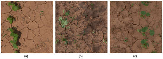
Figure 2.
Example of images divided to 2048 × 2048 in (a), (b), and (c).
3.2. Camera Characterization
To simulate the image formation pipeline with various types of image degradation, it is necessary to know the inherent camera characteristics so that the degradation can be introduced precisely, and the result can be reported quantitatively for future comparison. We characterized the point spread function, noise, gain, and color transformation matrix of the camera and the lens system using the raw images. Point spread function was estimated as a 2D Gaussian distribution by the slant edge method proposed by Fan et al. [30] using an image of a slant edge landmark taken at the beginning of each data collection (Figure 3). Noise and gain estimation was performed following the method proposed by Healey and Kondepudy [25]. Since it is difficult to estimate SNR of each pixel for a moving camera, we instead report SNR for the whole image dataset using the mean pixel intensity of all the pixel values in the dataset.
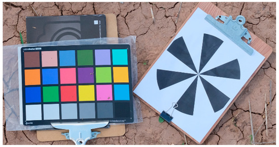
Figure 3.
An example of the ColorChecker and the slant edge landmark image taken by the camera before data collection in the field, for estimating color transformation matrix and point spread function (PSF).
To ensure correct rendering of the images, we converted the raw images from the camera’s color space to the standard RGB (sRGB) space through the Commission Internationale d’Eclairage (CIE) XYZ space. For this purpose, we captured an image of an X-Rite ColorChecker the same way as in PSF estimation (Figure 3). The ColorChecker image was white balanced using the 18% gray patch on the ColorChecker (the fourth patch from left to right) as reference. We applied to the whole image the scaling factors that force the average intensities of the red and blue channels on the gray patch to be equal to the green channel. Furthermore, a 3 × 3 color transformation matrix [41] was estimated to convert the white-balanced RGB values to XYZ values. A least square estimation approach was adopted to obtain , using the mean pixel intensities for each of the 24 patches on the ColorChecker and their corresponding XYZ values [42]. The transformation matrix from XYZ space to linear sRGB space was obtained from [43].
3.3. Simulation
A reference image that perfectly reproduces scene irradiance is ideal for the simulation. Unfortunately, such reference does not exist since any raw image from digital cameras does not preserve all the information of the scene due to blurring, noise, and Bayer filtering. We consider the raw images we collected as “ground truth” on which all the simulations were conducted.
The final simulated output images were generated from the raw images processed through the steps shown in Figure 1. We first subtracted the black level from the raw images and white-balanced them using the scaling factors calculated during the color transformation estimation process (Section 3.2). The images were then demosaicked using the nearest neighborhood interpolation method [44,45]. After demosaicking, the color transformation matrix was applied to convert the images from camera RGB space to XYZ space. Eventually, the images were converted to linear sRGB space and encoded by a tone response curve with gamma equal to 2.4. All the simulated images went through the same process except for the steps where degradation or denoising was introduced. The output images without any degradation or denoising were used as the baseline. Example images of the simulations are shown in Figure 4 and Figure 5.
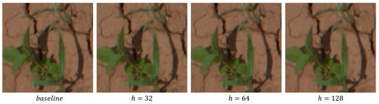
Figure 4.
Example of simulated images at denoising levels of = 32, 64, and 128, in comparison to the baseline.
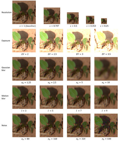
Figure 5.
Zoomed-in view of simulation results for resolution, exposure, Gaussian blur, motion blur, and noise.
3.3.1. Denoise
Convolutional kernels applied to the images for our blur simulations will inevitably reduce the overall pixel noise levels [46]. To confirm that denoising will not alter CNN performance, the non-local means algorithm proposed by Darbon et al. [47] was used to denoise the raw images in this experiment. The principle of this algorithm is to search in a window for patches that are similar enough to the patch of interest and then average the pixel values centered at resembling patches. We set the size of patch and search window at 7 × 7 and 21 × 21 pixels, respectively. The parameter that controls the weights of pixels with different similarity, , was tested at three levels: 32, 64, and 128. A higher results in a smoother but more blurred image (Figure 4).
3.3.2. Resolution
For a detector array with a given size, the pixel number is inversely related to pixel size. Our simulation of image resolution was analogous to replacing the original detector array by an array with the same array size, but bigger pixel size. The raw images were first demosaicked which were then resized using the box sampling algorithm [48]. Box sampling considers the target pixel as a box on the original image and calculates the average of all pixels inside the box weighted by their area within the box. Eventually each channel was sub-sampled according to the camera’s Bayer array pattern. The rest of the postprocessing steps were identical to that of the baseline images. Scale factor was set to 0.707, 0.5, 0.353, and 0.25 in our experiment.
3.3.3. Overexposure
An image may be described as overexposed when it loses highlight details [49,50]. In principle, we can set up an experiment to study how exposure affects CNN by changing shutter speed or aperture for the same scene. However, the drawback with this approach is that SNR also gets changed, making it difficult to isolate SNR effect from exposure effect. Thus, we simulated exposure in the postprocessing pipeline using the following function:
where is the saturated intensity value allowed by the bit depth of the image. In this experiment, exposure values (EV) of 2, 2.5, 3, and 3.5 were used. The resulting percentage of saturated pixels for is shown in Table 1.

Table 1.
Percentage of saturated pixels in each channel resulting from exposure simulation for with EV values of 2, 2.5, 3, and 3.5.
3.3.4. Gaussian Blur
The PSF resulting from lens imperfections, defocus, and the physics of light diffraction limit were approximated using 2D Gaussian blur [28,29,30,51]. The raw images were convoluted with 2D Gaussian kernels at four variance levels to simulate the effect of different PSFs. However, this will inevitably alter the variance of noise in each pixel and has similar effect as denoising [46]. As shown in the result of denoise simulation, the performance of CNN stays stable within a wide range of denoise levels. It can be assumed that reduction of noise variance by 2D Gaussian kernels will not significantly alter the performance of CNN. The 2D Gaussian kernels were applied with standard deviations () at 1.25, 2.5, 5, and 10. The resulting standard deviation of PSFs is shown in Table 2.
Table 2.
The standard deviations of the resulting PSFs after applying 2D Gaussian kernels to the raw images on top of the inherent image PSF.
3.3.5. Motion Blur
A motion blurred image is resulted from object or camera movement during exposure and can be in the form of translation, rotation, or sudden scaling [52]. In this research, we only focused on the translation blur as it is the most common form in weed mapping. The raw images were convoluted by 1D uniform kernels with different lengths to simulate the effect of linear motion blur [52]. The length of the 1D uniform kernels was set to 3, 5, 7, and 9 pixels. The inherent motion blur resulting from the drone movement can be ignored, as it is only equivalent to a ½ pixel long kernel, much smaller than the kernel length used for simulation.
3.3.6. Noise
A Poisson distribution is well approximated by a Gaussian distribution according to the Central Limit Theorem. The combined noise of a camera was simulated by a zero mean additive Gaussian noise and different levels of SNR were achieved by varying the variance of the Gaussian noise. The same was applied to all the three channels. The noise was added with at 80, 160, 320, and 640 to the raw images. The resulting SNR for channel was reported as:
where and are the estimated gain and noise, and is the mean pixel intensity of the whole dataset (Table 3).
Table 3.
Signal-to-noise ratio (SNR) resulting from adding Gaussian noise to the raw images with standard deviation at 80, 160, 320, and 640, respectively.
3.4. Image Annotation
Since the simulated images have a dimension of 11,648 × 8736, which is too large for neural network training, the images were divided into 2048 × 2048 patches. The resulting image sets were denoted as , , and Both bounding box and polygon annotation were performed on the divided images. The plant types in the image set were grouped into five categories: cotton, soybean, morningglory, grasses, and others. Although there were several grass species, they were grouped into a single category since they were hardly distinguishable in the images. The last category contains several weed species, but only makes up less than 3% of the total plant instances. A total of 1485 images were annotated for , 500 for , and 500 for . The composition and the size distribution of the annotated bounding box for the three lighting conditions were almost identical (Figure 6).
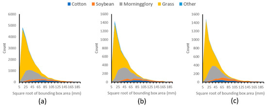
Figure 6.
Plant composition and bounding box size distribution of the annotated images for the three lighting conditions: (a) sunny around noon, (b) sunny around sunset, and (c) cloudy.
3.5. Neural Network Training and Evaluation
We trained and tested CNN models for three situations: (1) training and testing images have the same quality; (2) training and testing images have quality inconsistency; (3) training and testing images have light inconsistency. For the first and second situations, simulation was only performed on the 1485 images. images were split into 80% training set and 20% testing set. Two scenarios were considered for the second situation, the first being that the training images have higher quality than the testing images, the second being the opposite. In the first scenario, we trained a CNN model using the baseline images and tested on the degraded images. In the second scenario, we trained CNNs using images with specific degradations and tested on the baseline images. For image light consistency study, training sets were assembled with different number of images from , , and . Trained CNNs by the assembled training sets were then tested on 500 images that were not used for training. All training and testing were performed on a NVIDIA GeForce RTX 2080Ti GPU (graphics processing unit) with PyTorch framework [53]. Images were augmented only by random horizontal flipping during training.
We adopted a standard Faster R-CNN model with ResNet50 + FPN backbone [37,40]. The Faster R-CNN model was trained using transfer learning with the weights pretrained by Microsoft Common Objects in Context (COCO) train2017 images, a public dataset containing millions of images spanning 80 classes [54]. Stochastic gradient descent (SGD) optimizer [55] with a learning rate of 0.0005 and a batch size of 2 was chosen to minimize the loss function. Training stopped at 11,880 iterations when there was no further improvement of CNN performance. The sizes of anchor boxes were set to 322, 642, 1282, 2562 and 5122 with aspect ratio at 0.5, 1.0 and 2.0. The size of anchor boxes was scaled accordingly when testing the impact of resolution. Mask R-CNN provides both bounding box and instance segmentation prediction, but we only reported its instance segmentation performance as the bounding box prediction of Mask R-CNN and Faster R-CNN has a very similar trend. The same training strategy was adopted for Mask R-CNN.
The Deeplab-v3 model was used with the ResNet50 backbone for semantic segmentation [39]. The weights were pretrained by a subset of COCO train2017 images on the 20 categories that were present in the Pascal VOC dataset [56]. Each 2048 × 2048 image was further divided into four during training. The SGD optimizer [55] was adopted with a learning rate of 0.005 and a batch size of 2 to minimize the cross-entropy loss function. The model was trained for 6 epochs, each with 2376 iterations. Because of the imbalance of pixel number for each category, we used weighted loss for training, by setting the initial weights at 0.1, 1.0, 1.0, 1.0, 1.0, and 10 for background, cotton, soybean, morning glory, grass, and other, respectively. The weight of the background was adjusted to 0.5 after 2 epochs and to 1.0 again after another 2 epochs.
3.6. Metrics
For object detection and instance segmentation, we presented the results following the standard COCO-style average precision (AP). We reported AP for each plant category and also the mean AP (mAP) averaged from categorical AP. In addition, to examine CNN performance on plants with different sizes, the plants were grouped by bounding box area into the range of 0–102 mm2, 102–202 mm2, 202–402 mm2, 402–802 mm2, 802–1602 mm2, and >1602 mm2, corresponding to 0–36.52, 36.52–732, 732–1462, 1462–2922, 2922–5842, and >5842 pixels. AP were then calculated for each area range. For semantic segmentation, intersection over union (IoU) between the predicted mask and the ground truth mask of all the testing images were reported for each category. The ground truth mask was generated from the polygon annotation. The average of categorical IoU, mIoU, was also reported.
4. Results and Discussion
4.1. Effects of Image Denoising
In the experiment, we kept the size of comparing patch and search window the same but changed the parameter to control the amount of denoising. The image with shows a significant reduction of noise but tends to over-smooth the texture of the leaves and soil. However, the overall AP for object detection and instance segmentation was very close to the baseline (Figure 7). The same trend was observed in the semantic segmentation performance of Deeplab-v3. These results indicate that the denoising algorithm, even though it makes the images more visually appealing, does not significantly influence the performance of Faster Region-based CNN (R-CNN), Mask R-CNN and Deeplab-v3. It can also be safely assumed that the denoising effect of the kernels used in Gaussian blur and motion blur simulations will not significantly alter CNN performance.
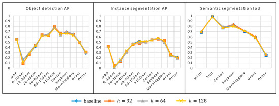
Figure 7.
Influence of image denoising on the performance of Faster R-CNN for object detection, of Mask R-CNN for instance segmentation, and of Deeplab-v3 for semantic segmentation.
4.2. Effects of Image Degradation
Training and testing of Faster R-CNN, Mask R-CNN and Deeplab-v3 were conducted on the images with the same degradation type and level. In general, the performance of Faster R-CNN and Mask R-CNN tends to decrease with the increase of the degradation levels (Figure 8). In contrast, Deeplab-v3 is more tolerant to image degradation.
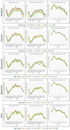
Figure 8.
The influence of resolution, overexposure, Gaussian blur, motion blur, and noise on the performance of Faster R-CNN, Mask R-CNN and Deeplab-v3 for object detection, instance segmentation and semantic segmentation.
4.2.1. Resolution Reduction
Faster R-CNN and Mask R-CNN is sensitive to resolution reduction. The AP values dropped from 55% to 34% for object detection and from 42% to 25% for instance segmentation when the resolution dropped from 2048 × 2048 (baseline) to 512 × 512, equivalent to a drop of spatial resolution from 0.27 mm/pixel to 1.10 mm/pixel. The influence of resolution can also be seen in the trend for AP from small to large plants. In the baseline dataset, object detection AP increased from 17% for plants smaller than 102 mm2 to 79% for plants larger than 1602 mm2. The same trend was also observed in the instance segmentation AP and semantic segmentation IoU.
4.2.2. Exposure
The red channel had the highest average pixel intensities in our dataset, followed by the green and the blue channels (Table 1). When EV increased, the red channel was the first channel with many pixels reaching saturation. However, the loss in highlight details of the red channel did not impact Faster R-CNN and Mask R-CNN performance. This is partially because most of the pixels with high red intensities were soil and the loss of information in the soil pixels did not affect the detection and classification of the crops and weeds. The performance did not decrease significantly even when the EV was 2.5, although it resulted in about 20% highlight detail loss in the green channel. Significant performance loss occurred when there was 67% highlight detail loss in the green channel. This result indicated that Faster R-CNN and Mask R-CNN is moderately tolerant to detail loss due to overexposure, especially in the red channel. Furthermore, the Deeplab-v3 was slightly influence by the information loss due to overexposure, even when there was 83.0% information loss in the green channel.
4.2.3. Gaussian Blur
Gaussian blur resulted in large quality degradation visually. However, it did not largely affect the performance of instance segmentation until reached 10. It was also notable that the performance drop occurred most severely for cotton. This is probably an indication that the feature types utilized by Mask R-CNN were different across plant species. For cotton, it is likely that Mask R-CNN relied more heavily on leaf details which were mostly lost in the highly blurred images. The same also happened in the noise experiment. Similar to that of Mask R-CNN, performance degradation for Deeplab-v3 only happened when reached 10 but only at a smaller extent. The largest decrease in the semantic segmentation IoU was also observed in cotton.
4.2.4. Motion Blur
Motion blur had little effect on the performance of Faster R-CNN, Mask R-CNN and Deeeplab-v3. A slight reduction was observed when was set at 7. This motion blur level was the same as that observed with flying the drone at a height of 4.88 m and a speed of 7.8 m/s, with the shutter speed and focal length settings at 1/4000 s and 64 mm, respectively. This result indicates that weed mapping can be performed at a relatively high speed without losing mapping accuracy.
4.2.5. Noise
Both in the object detection and instance segmentation tasks, low levels of noise ( and ) added to the images did not significantly change the performance for different categories of plants, except for cotton. It was likely that noise masked the fine details of cotton leaves, which the Faster R-CNN and Mask R-CNN relied upon (Figure 5). A significant performance reduction was observed with Faster R-CNN and Mask R-CNN when was 640, with corresponding SNR values at 4.0, 5.1, and 2.3 respectively for the red, green, and blue channels. The Deeplab-v3 was less sensitive to noise, with the only exception of cotton pixels wherein the classification accuracies were noticeably reduced at .
4.3. Quality Inconsistency between Training and Testing Datasets
CNN training and testing are two asynchronous processes. In real-world applications, it is difficult to totally avoid the situation where the testing image quality differs from that of the training images. Therefore, it is important to study how the quality difference (higher or lower) between training and testing images can influence CNN performance. For the high-quality training images, CNNs were trained on the baseline images and applied to the images with various levels of quality degradation (Table 4). For the low-quality training images, the CNN models were trained on images with specific degradations and were then applied to the baseline images (Table 5).
Table 4.
Result of inference by convolutional neural network (CNN) models trained on baseline images and applied to testing images with various levels of image degradation.
Table 5.
Result of inference by CNN models trained on images with various levels of image degradations and applied to the baseline testing images.
Faster R-CNN and Mask R-CNN trained on the baseline images were very sensitive to the degraded testing images. The highest sensitivity was observed with resolution reduction; when the resolution decreased from 2048 × 2048 to 512 × 512, object detection AP reduced from 55.4% to 3.5% and instance segmentation AP reduced from 42.3% to 2.3%. Faster R-CNN and Mask R-CNN were also sensitive to the exposure inconsistencies between the training and testing images, especially when the exposure differences were high. In contrast, low levels of motion blur and noise had little effect on Faster R-CNN and Mask R-CNN predictions. Deeplab-v3, on the other hand, was the most susceptible to exposure inconsistency. All levels of overexposure resulted in very poor segmentation performance. This was probably due to the heavy reliance of Deeplab-v3 on color information. The performance of Deeplab-v3 was moderately sensitive to resolution reduction, Gaussian blur, and noise, much lesser than that of Faster R-CNN and Mask R-CNN. Motion blur in the testing images had the least impact on Deeplab-v3′s performance and did not seem to affect Deeplab-v3 at low levels.
When the quality of the training images was lower than the testing images, the performance of Faster R-CNN and Mask R-CNN was less impacted. Again, the highest sensitivity was observed with resolution reduction. Faster R-CNN and Mask R-CNN trained on overexposed images were more robust to exposure changes than models trained by images that were not overexposed. This is probably because the non-overexposed images have features that do not exist in the overexposed images. Faster R-CNN and Mask R-CNN trained with low levels of motion blur and noise achieved very close performance to models trained with baseline images. Distinctively, Deeplab-v3 trained at all levels of motion blur and noise achieved the same or even higher IoU than the model trained by the baseline images. This indicates that when noise and motion blur are expected to vary in the testing images, increasing these two degradations in the training images is a good strategy to guarantee Deeplab-v3 performance. Similar to Faster R-CNN and Mask R-CNN, Deeplab-v3 trained with overexposed images was more tolerant to changes in exposure.
4.4. Light Inconsistency between Training and Testing Datasets
Training image sets pertaining to , , were used to train the CNN models, which were then applied on 500 testing images to study the influence of light inconsistency on CNN performance. The number of images from each lighting condition is shown in Table 6. As expected, the highest performance was achieved when all the 500 training images were from . When the number of images were increased from 166 to 500 without including images from and , the object detection AP and instance segmentation AP increased from 43.2% and 33.4% to 50.1% and 39.4%, respectively. This indicates that increasing training images pertaining to the same lighting condition typically increases CNN performance. When images from and were included and the total training image number was kept at 500, the performance of Faster R-CNN and Mask R-CNN increased, but not as much as the increase provided by images from . The worst performance was observed in the CNN models trained from . Because of the huge plant appearance different between and (Figure 2), CNNs probability learned features in not applicable to images. In contrast, Deeplab-v3 did not benefit much from the inclusion of training images at different lighting conditions.
Table 6.
Influence of light inconsistency on the performance of CNN models.
4.5. Implications of the Study
The degree of image degradation and inconsistency to which the CNNs can withstand for object detection, semantic segmentation and instance segmentation established in this research can be used to guide the selection of camera parameters in weed mapping applications. For example, we can fly a drone at a speed up to 5.6 m/s without losing CNN performance when the height is at 4.88 m, the shutter speed at 1/4000s and the focal length at 64 mm. As another example, camera exposure settings that keep 20% information of the red channel and 80% of the green channel will not result in much CNN performance reduction. When computational power allows, it is beneficial to keep a high spatial resolution for detection and segmentation tasks. Sharp images are not required as CNNs are tolerant to blur until the standard deviation of PSF reaches 5 pixels. Images collected from a camera with SNR larger than 5 are likely to provide good CNN performance, indicating that weed mapping can be performed under poor lighting conditions.
Keeping image quality consistent is of vital importance for CNN-based weed mapping. In real applications, training image collection should be conducted with the camera settings the same as the settings expected in the real inference stage. If maintaining quality consistency is a challenge, one strategy to make CNN more robust is to collect images with slight overexposure, Gaussian blur, motion blur or noise for training. Alternatively, high-quality images can be purposely downgraded to various levels in the training stage, as proposed by Pei et al. [10]. Light consistency is another important factor to consider. Light source dramatically influences the appearance of plants and alters the features learnable by CNNs in the training stage. Colleting training and testing images at the same time of day with the same cloudiness is recommended when an artificial light source is not available. If light consistency is not achievable, collecting training images under several lighting conditions is a favorable workaround.
5. Conclusions
In this study, we simulated the most common image degradations observed in weed mapping applications through the image formation pipeline and explored the influence of these degradations on the performance of the three widely used CNN models, Faster R-CNN, Mask R-CNN and Deeplab-v3, for object detection, instance segmentation, and semantic segmentation, respectively. The degradations simulated in this study included resolution reduction, overexposure, Gaussian blur, motion blur, and noise.
Our simulation of image degradation was based on the raw images which inevitably contain noise and blur. Even though we tried to keep these degradations as little as possible in the raw images, they cannot be eliminated completely. Thus, the best CNN performance that can be achieved on perfect images is still unknown. In addition, we only tested weed mapping when the crops and weeds were still young. How CNNs perform in detecting and segmenting mature plants still need to be studied. It is also worth mentioning that we only studied the influence of individual degradations on the CNN performance. The interaction between different degradations is a topic for future research.
Author Contributions
Conceptualization: C.H., M.V.B., B.B.S., J.A.T.; funding acquisition, supervision, and project administration: M.V.B.; methodology, investigation, data analysis, and writing the original draft: C.H.; editing and revisions: all authors; All authors have read and agreed to the published version of the manuscript.
Funding
This study was funded in part by the USDA-NRCS-Conservation Innovation Grant (CIG) program (Award # NR213A750013G017).
Institutional Review Board Statement
Not applicable.
Informed Consent Statement
Not applicable.
Data Availability Statement
Not applicable.
Acknowledgments
The authors acknowledge field support provided by Daniel Hathcoat and Daniel Lavy.
Conflicts of Interest
The authors declare that no conflict of interest exist.
References
- Chen, Y.-R.; Chao, K.; Kim, M.S. Machine vision technology for agricultural applications. Comput. Electron. Agric. 2002, 36, 173–191. [Google Scholar] [CrossRef]
- Cubero, S.; Aleixos, N.; Moltó, E.; Gómez-Sanchis, J.; Blasco, J. Advances in machine vision applications for automatic inspection and quality evaluation of fruits and vegetables. Food Bioprocess Technol. 2011, 4, 487–504. [Google Scholar] [CrossRef]
- Patel, K.K.; Kar, A.; Jha, S.N.; Khan, M.A. Machine vision system: A tool for quality inspection of food and agricultural products. J. Food Sci. Technol. 2012, 49, 123–141. [Google Scholar] [CrossRef] [PubMed]
- Kamilaris, A.; Prenafeta-Boldú, F.X. A review of the use of convolutional neural networks in agriculture. J. Agric. Sci. 2018, 156, 312–322. [Google Scholar] [CrossRef]
- Gao, J.; French, A.P.; Pound, M.P.; He, Y.; Pridmore, T.P.; Pieters, J.G. Deep convolutional neural networks for image-based Convolvulus sepium detection in sugar beet fields. Plant Methods 2020, 16, 1–12. [Google Scholar] [CrossRef]
- Dodge, S.; Karam, L. Understanding how image quality affects deep neural networks. In Proceedings of the 2016 Eighth International Conference on Quality of Multimedia Experience (QoMEX), Lisbon, Portugal, 6–8 June 2016. [Google Scholar]
- Karahan, S.; Yildirum, M.K.; Kirtac, K.; Rende, F.S.; Butun, G.; Ekenel, H.K. How image degradations affect deep CNN-based face recognition? In Proceedings of the 2016 International Conference of the Biometrics Special Interest Group (BIOSIG), Darmstadt, Germany, 21–23 September 2016. [Google Scholar]
- Dodge, S.; Karam, L. A study and comparison of human and deep learning recognition performance under visual distortions. In Proceedings of the 2017 26th International Conference on Computer Communication and Networks (ICCCN), Vancouver, Canada, 31 July–3 August 2017. [Google Scholar]
- Zhou, Y.; Liu, D.; Huang, T. Survey of face detection on low-quality images. In Proceedings of the 2018 13th IEEE International Conference on Automatic Face & Gesture Recognition (FG 2018), Xi’an, China, 15–19 May 2018. [Google Scholar]
- Pei, Y.; Huang, Y.; Zou, Q.; Zhang, X.; Wang, S. Effects of image degradation and degradation removal to CNN-based image classification. IEEE Trans. Pattern Anal. Mach. Intell. 2019, 43, 1239–1253. [Google Scholar] [CrossRef]
- Debevec, P.E.; Malik, J. Recovering high dynamic range radiance maps from photographs. ACM SIGGRAPH 2008, 2008, 1–10. [Google Scholar]
- Harold, R.M. An introduction to appearance analysis. GATF World 2001, 13, 5–12. [Google Scholar]
- Liu, Y.C.; Chan, W.H.; Chen, Y.Q. Automatic white balance for digital still camera. IEEE Trans. Consum. Electron. 1995, 41, 460–466. [Google Scholar]
- Akenine-Möller, T.; Haines, E.; Hoffman, N. Real-Time Rendering, 4th ed.; CRC Press: Boca Raton, FL, USA, 2019; pp. 377–391. [Google Scholar]
- Peng, B.; Yang, H.; Li, D.; Zhang, Z. An empirical study of face recognition under variations. In Proceedings of the 2018 13th IEEE International Conference on Automatic Face & Gesture Recognition (FG 2018), Xi’an, China, 15–19 May 2018. [Google Scholar]
- Gao, X.; Li, S.Z.; Liu, R.; Zhang, P. Standardization of face image sample quality. International Conference on Biometrics; Springer: Berlin/Heidelberg, Germany, 2007. [Google Scholar]
- Bağcı, U.; Udupa, J.K.; Bai, L. The role of intensity standardization in medical image registration. Pattern Recognit. Lett. 2010, 31, 315–323. [Google Scholar] [CrossRef]
- Chebrolu, N.; Lottes, P.; Schaefer, A.; Winterhalter, W.; Burgard, W.; Stachniss, C. Agricultural robot dataset for plant classification, localization and mapping on sugar beet fields. Int. J. Robot. Res. 2017, 36, 1045–1052. [Google Scholar] [CrossRef]
- Kounalakis, T.; Malinowski, M.J.; Chelini, L.; Triantafyllidis, G.A.; Nalpantidis, L. A robotic system employing deep learning for visual recognition and detection of weeds in grasslands. In Proceedings of the 2018 IEEE International Conference on Imaging Systems and Techniques (IST), Krakow, Poland, 16–18 October 2018. [Google Scholar]
- Olsen, A. Konovalov, D.A.; Philippa, B.; Ridd, P.; Wood, J.C.; Johns, J.; Banks, W.; Girgenti, B.; Kenny, O.; Whinney, J.; Calvert, B.; Azghadi, M.R.; White, R.D. DeepWeeds: A multiclass weed species image dataset for deep learning. Sci. Rep. 2019, 9, 1–12. [Google Scholar]
- Farrell, J.E.; Xiao, F.; Catrysse, P.B.; Wandell, B.A. A simulation tool for evaluating digital camera image quality. In Proceedings of the Electronic Imaging Symposium, San Jose, CA, USA, 18–22 January 2004. [Google Scholar]
- Tsin, Y.; Ramesh, V.; Kanade, T. Statistical calibration of CCD imaging process. In Proceedings of the Eighth IEEE International Conference on Computer Vision, Vancouver, Canada, 7–14 July 2001. [Google Scholar]
- Liu, C.; Freeman, W.T.; Szeliski, R.; Kang, S.B. Noise estimation from a single image. In Proceedings of the 2006 IEEE Computer Society Conference on Computer Vision and Pattern Recognition (CVPR’06), New York, NY, USA, 17–22 June 2006. [Google Scholar]
- Sumner, R. Processing RAW Images in MATLAB; Department of Electrical Engineering, University of California Sata Cruz: Santa Cruz, CA, USA, 2014. [Google Scholar]
- Healey, G.E.; Kondepudy, R. Radiometric CCD camera calibration and noise estimation. IEEE Trans. Pattern Anal. Mach. Intell. 1994, 16, 267–276. [Google Scholar] [CrossRef]
- Farrell, J.E.; Catrysse, P.B.; Wandell, B.A. Digital camera simulation. Appl. Opt. 2012, 51, A80–A90. [Google Scholar] [CrossRef]
- Catrysse, P.B.; Wandell, B.A. Roadmap for CMOS image sensors: Moore meets Planck and Sommerfeld. In Proceedings of the Electronic Imaging, San Jose, CA, USA, 16–20 January 2005. [Google Scholar]
- Hu, H.; De Haan, G. Low cost robust blur estimator. In Proceedings of the 2006 International Conference on Image Processing, Atlanta, GA, USA, 8–11 October 2006. [Google Scholar]
- Claxton, C.D.; Staunton, R.C. Measurement of the point-spread function of a noisy imaging system. J. Opt. Soc. Am. A 2008, 25, 159–170. [Google Scholar] [CrossRef]
- Fan, C.; Li, G.; Tao, C. Slant edge method for point spread function estimation. Appl. Opt. 2015, 54, 4097–4103. [Google Scholar] [CrossRef]
- Ramanath, R.; Snyder, W.E.; Yoo, Y.; Drew, M.S. Color image processing pipeline. IEEE Signal Process. Mag. 2005, 22, 34–43. [Google Scholar] [CrossRef]
- European Machine Vision Association. EMVA standard 1288, standard for characterization of image sensors and cameras. Release 2016, 3, 6–27. [Google Scholar]
- Frank, J.; Al-Ali, L. Signal-to-noise ratio of electron micrographs obtained by cross correlation. Nature 1975, 256, 376–379. [Google Scholar] [CrossRef]
- Carlsson, K. Imaging Physics; KTH Applied Physics Department: Stockholm, Sweden, 2009. [Google Scholar]
- Kao, W.C.; Wang, S.H.; Chen, L.Y.; Lin, S.Y. Design considerations of color image processing pipeline for digital cameras. IEEE Trans. Consum. Electron. 2006, 52, 1144–1152. [Google Scholar] [CrossRef]
- Ren, Y.; Cheng, X. Review of convolutional neural network optimization and training in image processing. In Proceedings of the Tenth International Symposium on Precision Engineering Measurements and Instrumentation, Kunming, China, 8–10 August 2018. [Google Scholar]
- Ren, S.; He, K.; Girshick, R.; Sun, J. Faster R-CNN: Towards real-time object detection with region proposal networks. IEEE Trans. Pattern Anal. Mach. Intell. 2015, 39, 1137–1149. [Google Scholar] [CrossRef]
- Garcia-Garcia, A.; Orts-Escolano, S.; Oprea, S.; Villena-Martinez, V.; Garcia-Rodriguez, J. A review on deep learning techniques applied to semantic segmentation. arXiv 2017, arXiv:1704.06857. [Google Scholar]
- Chen, L.C.; Papandreou, G.; Schroff, F.; Adam, H. Rethinking atrous convolution for semantic image segmentation. arXiv 2017, arXiv:1706.05587. [Google Scholar]
- He, K.; Gkioxari, G.; Dollár, P.; Girshick, R. Mask R-CNN. In Proceedings of the IEEE International Conference on Computer Vision, Venice, Italy, 22–29 October 2017. [Google Scholar]
- Varghese, D.; Wanat, R.; Mantiuk, R.K. Colorimetric calibration of high dynamic range images with a ColorChecker chart. In Proceedings of the HDRi 2014: Second International Conference and SME Workshop on HDR Imaging, Sarajevo, Bosnia and Herzegovina, 4–5 March 2014; 2014. [Google Scholar]
- Pascale, D. RGB Coordinates of the Macbeth Color Checker; The BabelColor Company: Montreal, Canada, 2006. [Google Scholar]
- Lindbloom, B.J.; RGB/XYZ Matrices. Bruce Lindbloom’s Web Site. Available online: http://www.brucelindbloom.com/index.html?Eqn_RGB_XYZ_Matrix.html (accessed on 23 January 2021).
- Longere, P.; Zhang, X.; Delahunt, P.B.; Brainard, D.H. Perceptual assessment of demosaicing algorithm performance. Proc. IEEE 2002, 90, 123–132. [Google Scholar] [CrossRef]
- Rani, S.K.; Hans, W.J. FPGA implementation of bilinear interpolation algorithm for CFA demosaicing. In Proceedings of the 2013 International Conference on Communication and Signal Processing, Melmaruvathur, India, 3–5 April 2013. [Google Scholar]
- Gonzales, R.C.; Woods, R.E. Digital image processing, 4th ed.; Pearson: Sholinganallur, Chennai, 2018; pp. 317–368. [Google Scholar]
- Darbon, J.; Cunha, A.; Chan, T.F.; Osher, S.; Jensen, G.J. Fast nonlocal filtering applied to electron cryomicroscopy. In Proceedings of the 2008 5th IEEE International Symposium on Biomedical Imaging: From Nano to Macro, Paris, France, 14–17 May 2008. [Google Scholar]
- Image Scaling Wikipedia. Available online: https://en.wikipedia.org/wiki/Image_scaling (accessed on 23 January 2021).
- Guo, D.; Cheng, Y.; Zhuo, S.; Sim, T. Correcting over-exposure in photographs. In Proceedings of the 2010 IEEE Computer Society Conference on Computer Vision and Pattern Recognition, San Francisco, CA, USA, 13–18 June 2010. [Google Scholar]
- Präkel, D. Photography Exposure, 2nd ed.; Bloomsbury Publishing: New York, NY, USA, 2016; pp. 37–38. [Google Scholar]
- Zhang, B.; Zerubia, J.; Olivo-Marin, J. Gaussian approximations of fluorescence microscope point-spread function models. Appl. Opt. 2007, 46, 1819–1829. [Google Scholar] [CrossRef] [PubMed]
- Tiwari, S.; Shukla, V.P.; Singh, A.K.; Biradar, S.R. Review of motion blur estimation techniques. J. Image Graph. 2013, 1, 176–184. [Google Scholar] [CrossRef]
- Paszke, A.; Gross, S.; Massa, F.; Lerer, A.; Bradbury, J.; Chanan, G.; Killeen, T. PyTorch: An imperative style, high-performance deep learning library. Adv. Neural Inf. Process. Syst. 2019, 32, 8026–8037. [Google Scholar]
- Lin, T.Y.; Maire, M.; Belongie, S.; Hays, J.; Perona, P.; Ramanan, D.; Dollár, P.; Zitnick, C.L. Microsoft COCO: Common objects in context. In European Conference on Computer Vision; Springer: Cham, Switzerland, 2014. [Google Scholar]
- Ruder, S. An overview of gradient descent optimization algorithms. arXiv 2016, arXiv:1609.04747. [Google Scholar]
- Everingham, M.; Eslami, S.A.; Van Gool, L.; Williams, C.K.; Winn, J.; Zisserman, A. The pascal visual object classes challenge: A retrospective. Int. J. Comput. Vis. 2015, 111, 98–136. [Google Scholar] [CrossRef]


Publisher’s Note: MDPI stays neutral with regard to jurisdictional claims in published maps and institutional affiliations. |
© 2021 by the authors. Licensee MDPI, Basel, Switzerland. This article is an open access article distributed under the terms and conditions of the Creative Commons Attribution (CC BY) license (https://creativecommons.org/licenses/by/4.0/).