Article

Improved Estimation of Aboveground Biomass of Disturbed Grassland through Including Bare Ground and Grazing Intensity

1
School of Environment, The University of Auckland, Auckland 1142, New Zealand
2
State Key Laboratory of Plateau Ecology and Agriculture, College of Agriculture and Animal Husbandry, Qinghai University, Xining 810016, China
*
Author to whom correspondence should be addressed.
Remote Sens. 2021, 13(11), 2105; https://doi.org/10.3390/rs13112105
Submission received: 20 April 2021 / Revised: 18 May 2021 / Accepted: 24 May 2021 / Published: 27 May 2021
(This article belongs to the Section Forest Remote Sensing)

Abstract

:
Accurate approaches to aboveground biomass (AGB) estimation are required to support appraisal of the effectiveness of land use measures, which seek to protect grazing-adapted grasslands atop the Qinghai-Tibet Plateau (QTP). This methodological study assesses the effectiveness of one commonly used visible band vegetation index, Red Green Blue Vegetation Index (RGBVI), obtained from unmanned aerial vehicle (UAV), in estimating AGB timely and accurately at the local scale, seeking to improve the estimation accuracy by taking into account in situ collected information on disturbed grassland. Particular emphasis is placed upon the mapping and quantification of areas disturbed by grazing (simulated via mowing) and plateau pika (Ochotona curzoniae) that have led to the emergence of bare ground. The initial model involving only RGBVI performed poorly in AGB estimation by underestimating high AGB by around 10% and overestimating low AGB by about 10%. The estimation model was modified by the mowing intensity ratio and bare ground metrics. The former almost doubled the estimation accuracy from R2 = 0.44 to 0.81. However, this modification caused the bare ground AGB to be overestimated by about 38 and 19 g m−2 for 2018 and 2019, respectively. Although further modification of the model by bare ground metrics improved the accuracy slightly to 0.88, it markedly reduced the overestimation of low AGB values. It is recommended that grazing intensity be incorporated into the micro-scale estimation of AGB, together with the bare ground modification metrics, especially for severely disturbed meadows with a sizable portion of bare ground.

Graphical Abstract

1. Introduction

Grasslands are vital ecosystems that occupy about 40% of the Earth’s surface [1]. With an area of about 2.5 million km2, grasslands atop the Qinghai-Tibet Plateau (QTP) provide an important grazing resource that supports the livelihood of local pastoralists [2]. Maintenance of grazing-adapted ecosystems is an integral part of long-term environmental protection programmes in this region [3]. In recent decades, climate change, overgrazing and rodents threaten this ecosystem [4,5]. Around 40% of grassland areas in the Sanjiangyuan region of the QTP have been subjected to fragmentation and degradation [6,7,8]. Essentially, the prospect for sustainable practices reflects the balance between changes to grassland productivity, on the one hand (i.e., net primary productivity; NPP), and impacts of land use practices, especially stocking rates, on the other [9,10]. Given the vast expanse of the landscapes and ecosystems in this region, research to date has emphasized the use of remotely sensed applications to appraise spatial and temporal variability in the patterns and rates of human impact upon the viability of grassland systems, with many studies seeking to differentiate the impacts of climate change from those of human activities on broad-scale trends in NPP [11,12,13,14,15,16,17]. Ultimately, however, the processes that drive land use impacts upon grassland productivity, and associated measures of environmental degradation, reflect local-scale land use practices [18,19,20]. This presents significant challenges in the generation of systematic databases and insights that build upon data of sufficient resolution to track (and interpret) local-scale variability, thereby informing land management practices at an appropriate scale. Timely and accurate monitoring of grassland vegetation productivity is required to support grassland management and restoration [21]. To date, most studies of grassland vegetation productivity are based upon broad-scale estimates [22,23,24,25]. However, tracking local-scale variability is the key to understanding the susceptibility of grassland vegetation dynamics, thereby underpinning efforts to balance livestock grazing intensity as a key part of grassland management strategies. This paper reports on the use of drone imagery as a tool to support such analyses.
Grassland aboveground biomass (AGB) is a reliable indicator of grassland ecosystem function and productivity, as well as grassland health [26,27,28]. AGB is highly sensitive to climate change, anthropogenic activities and rodent disturbance; it is commonly estimated via field sampling and remote sensing. The former is destructive and requires subjective visual assessment of grass cover. It is also time-consuming and labour-intensive and, hence, impractical for large-scale estimation [29,30,31]. In contrast, the latter is able to provide a bird-eye coverage of large areas with a high efficiency and accuracy [32]. With the assistance of in situ samples collected at a limited number of sites concurrently with the acquisition of remote sensing images [33], this method enables rapid, highly accurate and up-to-date estimation of AGB [34,35,36,37]. Grassland AGB can be estimated by various processing methods of the rich spectral information of remote sensing imagery. One common processing method is known as vegetation indexing (VI), which can effectively capture vegetation conditions and provide a useful approach to monitor grassland biomass [38]. It could be derived from the near-infrared bands and visible bands (red, green and blue bands). Although drone images commonly lack the critical infrared bands, visible band VIs from drone images such as the Red Green Blue Vegetation Index (RGBVI) [39,40] achieved an accuracy higher than 87.73% at 30 m above the ground, and 83.74% at 60 m above the ground in mapping the vegetation fraction of crop fields [41]. Acquired at an altitude of less than 100 m, unmanned aerial vehicle (UAV) images offer great possibilities in monitoring grassland health [42,43]. So far, UAV has shown a great promise in estimating terrestrial vegetation productivity [44,45,46,47]. However, remote-sensing-based methods had the limitations in reflecting the three-dimensional (3D) structure of vegetation, because images just show the aerial view of the vegetation from above [48]. With the rapid development in digital photogrammetric techniques, multi-view stereopsis methods such as structure from motion could compute 3D point clouds by overlapping 2D images acquired from multiple angles around the target [49,50,51]. However, this method has no potentiality to build the 3D structure for the huge pastures on the QTP. Although light detection and ranging (LiDAR) and terrestrial laser scanner (TLS) enable 3D surfaces to be constructed [52,53,54], they are not suitable for grassland of a low stature that requires high-density point clouds. They will incur a high cost for large pastoral areas [53]. In reality, plant vertical information such as height is not a reliable proxy of its AGB, but AGB bears a close relationship with stocking rate and grazing intensity (R2 = 0.72) [55,56]. Furthermore, the same grazing intensity could provide average vegetation height [57]. Thus, it may be possible to increase the accuracy of grassland AGB estimation by taking into account the vertical properties of grasses based on grazing intensity.
AGB estimation uncertainties can stem from bare ground, which is clearly visible on high-resolution UAV images. For instance, pika can create bare ground via burrowing and gnawing [58,59]. Such bare ground exerts significant influences on the spectral properties of vegetation canopies of arid grassland [60,61], thus degrading the estimation accuracy. Because VIs are sensitive to background factors, the soil background brightness could increase their value [62,63], thereby resulting in grassland AGB to be overestimated. At present, it remains unknown how the estimation accuracy can be improved via considering the effect of bare ground caused by pika disturbance.
In order to fill the identified knowledge gaps, this study aims to estimate alpine meadow AGB from multi-temporal drone images at a micro-scale and improve estimation accuracy in relation to two types of external disturbances (mowing-simulated grazing and rodents). The specific objectives are (a) to develop a method for alpine grassland AGB estimation from fine-resolution drone images without radiometric calibration; (b) to evaluate the improvement in AGB estimation accuracy by taking into account the meadow conditions caused by disturbances; and (c) to evaluate the influence of bare ground on the AGB estimation accuracy.

2. Materials and Methods

2.1. Study Area

The study area is located in the Henan Mongolian Autonomous County in the eastern Sanjiangyuan Region on the QTP (Figure 1). At an average elevation of 3600 m above sea level, this area has a plateau continental climate, with annual temperature ranging from 9.2 to 14.6 °C, and annual precipitation ranging from 597.1 to 615.5 mm. There are 5982.29 km2 of available grassland in this county, 92.68% of which takes the form of typical alpine meadow. The grassland vegetation is dominated by Kobresia tibetica and has been affected by rodents and overgrazing [64,65], putting this area at the risk of degradation. The study site is located on a floodplain of the Yellow River with a gentle topography, and it suffers a moderate disturbance of pika (Ochotona curzoniae) and grazing.

2.2. Field Experiment and Data Collection

2.2.1. Setup of Experimental Plots

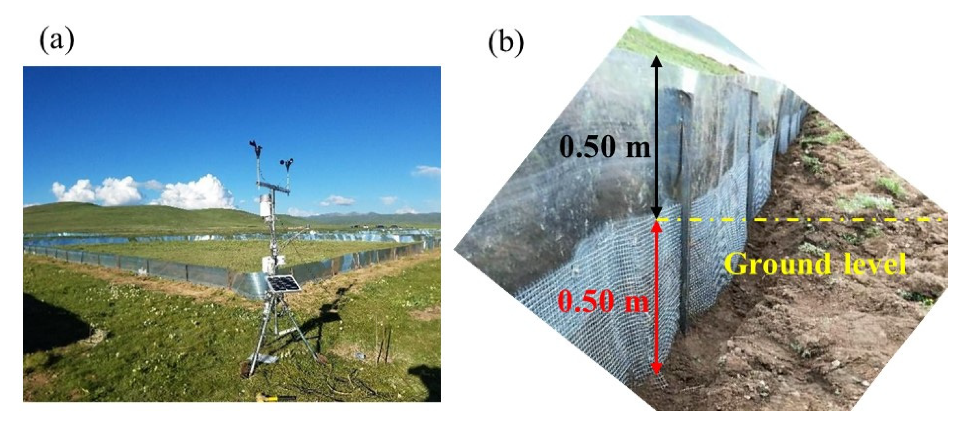
In total, 27 plots of 25 by 30 m were set up with a corridor of 5 m between neighbouring plots in a fenced site in June 2018 (Figure 1). A wire mesh fence was set 50 cm above the ground and extended about 50 cm beneath the surface, deeper than the approximate depth (20 to 30 cm) of pika burrowing so as to prevent pika intrusion into and roaming among the plots (Figure 2) [66,67]. All the plots were treated with three levels of disturbance (none, medium and high) for pika population and mowing intensity individually and jointly, resulting in nine treatments in total (Table 1). Each treatment was replicated three times. Spatially, the nine treatments of a given replica were randomly allocated to each of the three rows of plots (Figure 1).
Plateau pika used in this study is a small mammal with a body weight of 130–200 g, widely scattered in the alpine grassland of the QTP [68]. It affects grassland not only through directly devouring forage but also via burrowing and digging [69,70]. The intensity of pika disturbance was set with reference to the literature, namely, 200 individual ha−1 or 14 in a plot for strong disturbance (Ph) and 7 for medium disturbance (Pm) [71,72]. No pika (Pn) plots served as the reference. In each plot, traps were placed to eradicate the existing pika population one month prior to field sampling. Afterwards, poisoning was applied to each plot to exterminate any residual pika. More traps were placed outside the plots to collect pika before the experiment. Later, they were released to the pre-designated plots in accordance with the pre-determined intensity at a male–female ratio of 1:1 for Ph and 3:4 for Pm [73]. The pika population and gender in each plot were re-assessed in July 2019 to ensure that they still conformed to the required specifications. Any deviations from them were remedied by removing or supplementing pika to the affected plots as appropriate.
Livestock grazing was simulated via mowing twice a year in mid-July and mid-August. Mowing height could be used as a proxy for grazing intensity [74], as the same grazed pastures had a similar vegetation height [57]. So, mowing intensity was dictated by the mower blade height. Heavy grazing (Gh) was simulated by setting the blade at the extremely low level of 2 cm above the ground; the height was 12 cm for moderate grazing (Gm), which was about half of the plant height (24 cm). Gn was the reference treatment without mowing. The exact blade height was based on the one-third principle, namely, the clipped grass should not exceed one third of the plant height to reduce stress on the mown grass and to promote forage lateral growth [75].

2.2.2. UAV Images and Biomass Sampling

All experimental plots were photographed using an RGB digital camera (1 inch, 20 megapixel Complementary Metal Oxide Semiconductor sensor) aboard a Dajiang Phantom 4 UAV (Shenzhen Dajiang Baiwang Technology Co., Ltd., Shenzhen, China) in the auto mode in late August of 2018 and 2019. Acquired at a flying height of around 40 m above the ground, each drone image of a plot comprises 4864 × 3648 pixels (pixel size = 1 by 1 cm). The images were not radiometrically corrected, even though this can enhance the success of VI-based analyses [76]. This is permissible because VI can be reliably estimated from non-calibrated high-resolution images so long as they are obtained under the same radiometric conditions [77].
Within each plot, the location of the biomass-sampled quarter (1 by 1 m) was determined with reference to the plot fence, which was converted to local coordinates for quadrat demarcation on the drone images (Figure 1). To synchronize with the drone photographing, the plant material in one random quarter of the quadrat (formed by the two diagonal axes) was collected by clipping all the grasses to the ground level as closely as possible in 2018, and one of the remaining three quarters was harvested randomly in 2019. In total, 216 samples (27 plots by 8 quadrats) were collected each year. After all the non-plant materials were removed, the clipped fresh grasses were oven-dried until weights stabilized, and this weight was regarded as the ground truth biomass. Analysis of variance (ANOVA) and least significant difference were performed to test the differences in AGB between the treatments.

2.3. Data Processing

2.3.1. Bare Ground Mapping and RGBVI Calculation

Bare ground devoid of any biomass in a plot was mapped using the Support Vector Machine classifier in ArcMap 10.7, together with grassy meadow. This classifier is a spectral classification method involving supervised learning. It is based on an iterative process of calculating the n-dimensional classification to find the optimum hyperplane boundary, which can classify data with unknown statistical distributions by using small training sets successfully [78,79]. As bare ground is visible on the drone images, all the training samples were randomly selected by visual inspection. Two indicators, overall accuracy and Kappa coefficient, were used to indicate classification accuracy based on 150 randomly selected evaluation points [80,81].
As the fence of each plot was clearly visible in the drone images, it served as the ground control for geo-referencing the UAV image of a plot to a dimension of 25 by 30 m in ArcMap (Figure 1). The rectified image was clipped to 24.5 by 29.6 m to exclude the fence shadow, from which VI images were derived. These VIs were later used to estimate AGB from the 2018 and 2019 drone images separately to avoid any inconsistency in the illumination conditions between them. The Red Green Blue Vegetation Index (RGBVI) was used to estimate AGB in this study (Equation (1)); it has been successfully used for vegetation biomass estimation [82,83,84]. After the RGBVI calculation, pixels corresponding to the harvested quarter (0.25 m2) in each quadrat were extracted (about 250 in total) from the geo-referenced VI images via their coordinates determined from the distance to the plot border.
RGBVI = G R E E N × G R E E N B L U E × R E D G R E E N × G R E E N + B L U E × R E D

2.3.2. AGB Modelling

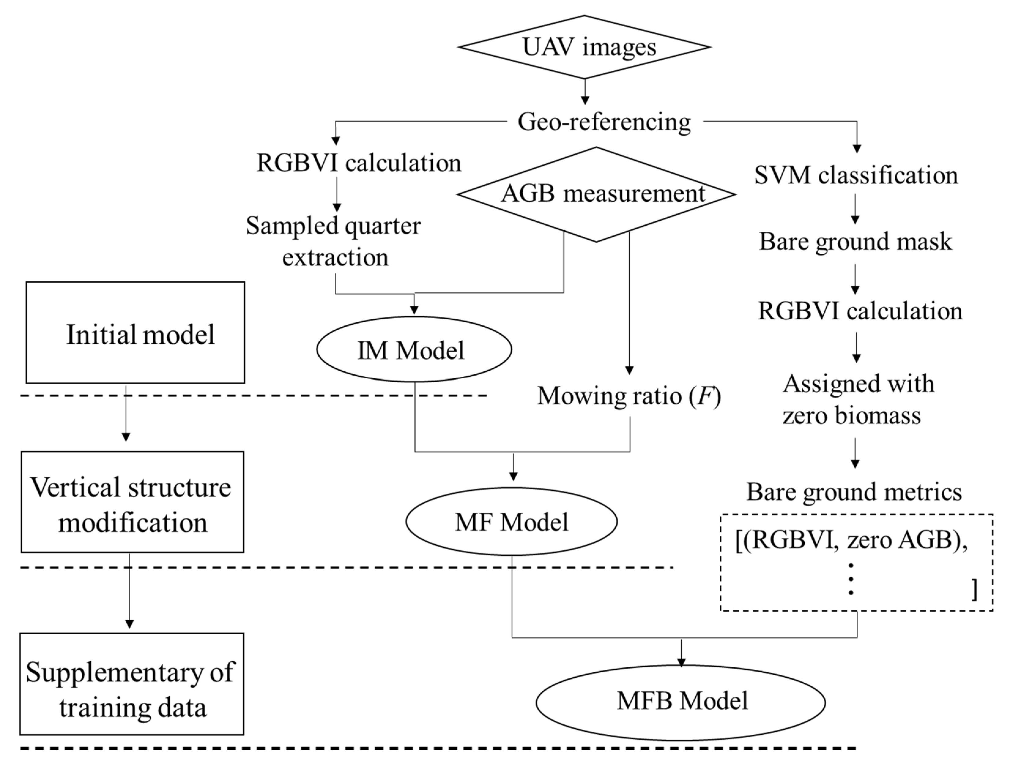
Three types of model were built in this study (Figure 3); separate regression models, both linear and second-order polynomial were built for the 2018 and 2019 images, and the best one was used to evaluate model performance. The initial model was constructed from the RGBVI values extracted from 216 pixels each year, during which the RGBVI value of the pixels falling into the same sampling quarter was averaged prior to its regression against the in situ measured AGB.
The initial model was modified by two ratios. The first is the mowing ratio (F) based on mowing intensity that was treated as a proxy for vegetation biomass. The mowing effect on the biomass removal was proportional to the removed biomass corresponding to the reference plots. It is calculated as:
F = i = 1 n B b i B
where n is the number of sample plots having the same mowing intensity; B is the averaged in situ measured AGB of the sampled quarter in the reference plots (PnGn), and b is the measured AGB of the sampled quarter in the plots of the same mowing intensity.
F was used to modify the RGBVI value:
M F = 1 m i = 1 m R G B V I i × ( 1 F t ) k
where t denotes one of the three mowing intensities; (1 − Ft)k is the biomass density factor, which can reflect the vertical properties of the grassland; k is a constant determined via non-linear regression (k = 4 produced the best result for the study area but could be slightly different for other areas).
The second ratio is the bare ground metrics. This modification was implemented by extracting the corresponding VI of bare ground pixels in a newly created mask layer and assigning a value of zero to them in the output metrics. These bare ground modification metrics were then used as the ground truth dataset, which can provide more modelling samples in model construction and validation. This metric was used as the supplementary training dataset based on the MF model to further improve the AGB estimation accuracy (Figure 3).
All models were validated using the “leave one out cross validation” (LOOCV) method. LOOCV can minimize the overfitting problem and provide an accurate assessment of model prediction strength, using each sample for validation and the rest for training [85,86]. The coefficient of determination (R2), root mean square error (RMSE) and mean error were employed to evaluate the over- or under-estimated biomass. The last was used to assess the model’s prediction errors to represent overestimations (positive number) and underestimations (negative number). The closer the mean error to zero, the more accurate the estimate.
RMSE = i = 1 n ( y i Y i ) 2 n 1
where yi and Yi are the measured and modelled AGB, respectively, and n is the total number of samples.
However, R2 has an inherent problem in explaining the additional input variables relating to the model outputs. The changes in the training dataset may cause the overfitting problem in the model. So, adjusted R2 is introduced to check whether the bare ground modification metrics improved model accuracy.

3. Results

3.1. Biomass Reference Data and Modification Assessment

3.1.1. Measured AGB and Mowing Modification Ratio (F)

The field measured AGB is statistically summarized in Table 2. Although the year of 2018 had more AGB than the year of 2019 (178.20 vs. 145.64 g m−2 on average), the control plots and intensively mowed plots had the maximum and minimum AGB, respectively, in both years. In the mowed plots, AGB dropped along with the mowing intensity, but pika disturbance had no such effect as the medium disturbance group had the lowest AGB. Moreover, the AGB of pika treated plots had a narrow range from 166.47 to 188.46 g m−2 than the mowed plots from 140.52 to 200.24 g m−2 in 2018. Furthermore, the latter varied significantly between disturbance severities while the former did not. This finding still held true in 2019. Figure 4 displayed the mowing intensity modification ratio (F) based on the field collected data, which had a value less than 0.4 in both 2018 and 2019. F of the reference plots was close to zero, and the moderately mowed plots had a slightly higher value of 0.11 and 0.14 in both years, respectively. The severely mowed plots had a value of 0.36 on average. The average value at each severity was used for model modification.

3.1.2. Bare Ground Modification Metrics

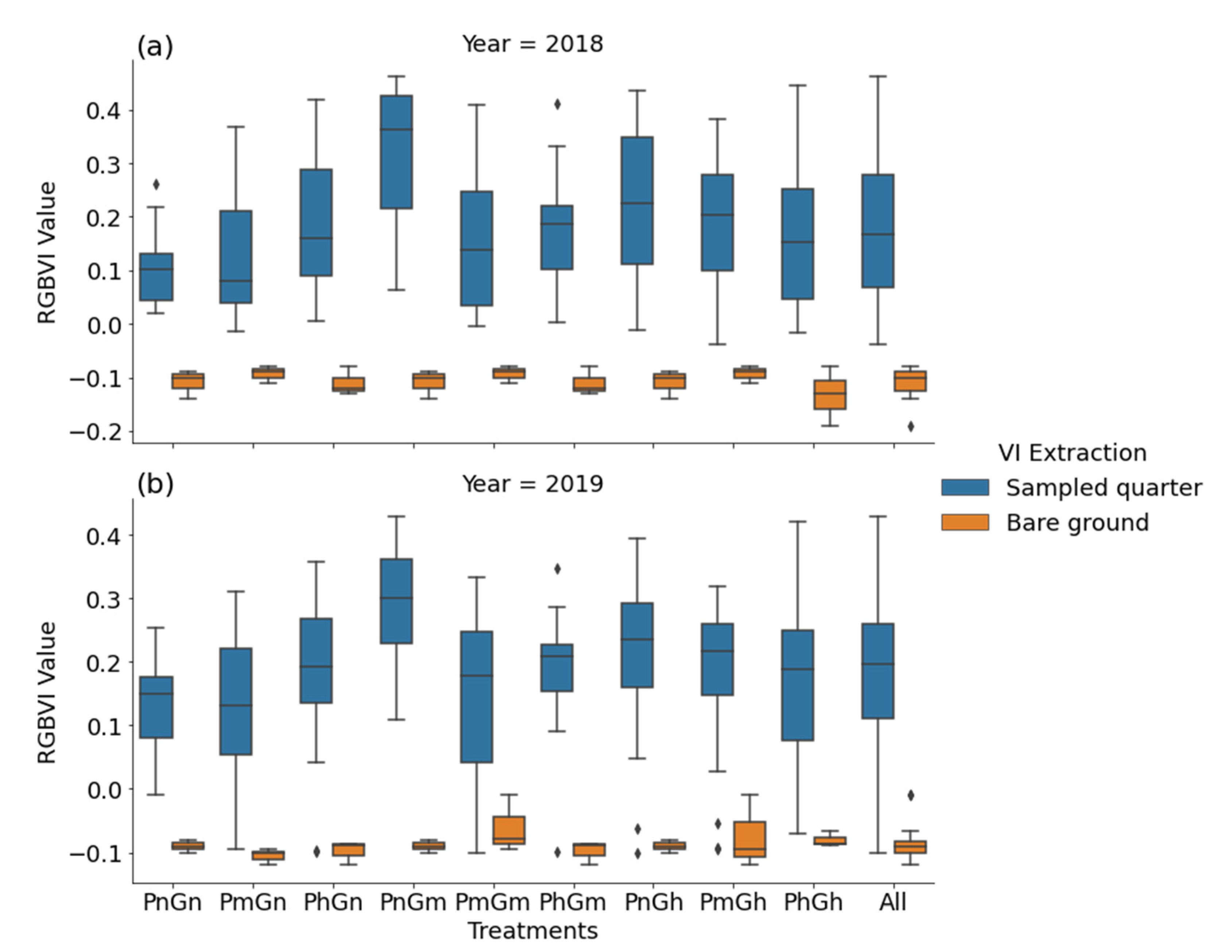
In order to assess the effect of bare ground on AGB estimation, bare ground in each plot has been mapped to an overall accuracy higher than 94.0% and a Kappa over 0.89. In 2018, the RGBVI of the sampled quarter was mainly positive ranging from −0.03 to 0.47 (Figure 5a). Only few negative RGBVI values were found, which still corresponded to the field measured AGB values (above zero), while bare ground had smaller RGBVI values, which were all negative numbers, without overlapping with the former. Although the sampled quarters had overlapping bare ground in 2019 (Figure 5b), their interquartile ranges were distinct.

3.1.3. Disturbance-Specific Models

The performance of the disturbance-specific models was evaluated based on the linear model for each disturbance severity (none, medium and high) using RGBVI and the measured AGB in both 2018 and 2019 (Figure 6). RGBVI had a close relationship with the measured AGB at all mowing severities, with an R2 around 0.70 in both years, while the reference groups had a lower accuracy less than 0.70 and 0.68, respectively (Figure 6a,c). However, the models of the pika-disturbed groups were much less accurate with R2 < 0.30. It is noteworthy that the lesser the mowing severity, the higher the measured AGB, but the rank of model reliability remains unchanged in both years. However, there were more negative VIs in the medium and severe groups (joint disturbances by mowing and pika) in 2019. Overall, mowing had significant impacts on the regression models, but not pika disturbance. This indicates the possibilities of improving the AGB estimation accuracy based on mowing intensity.

3.2. AGB Models and Accuracy

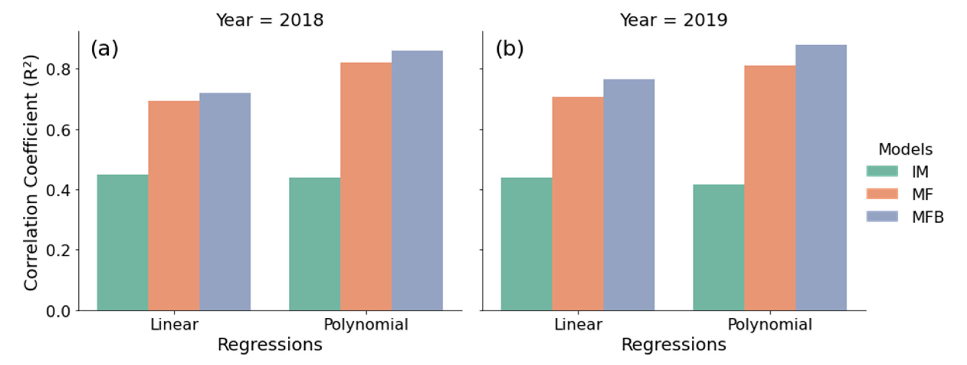
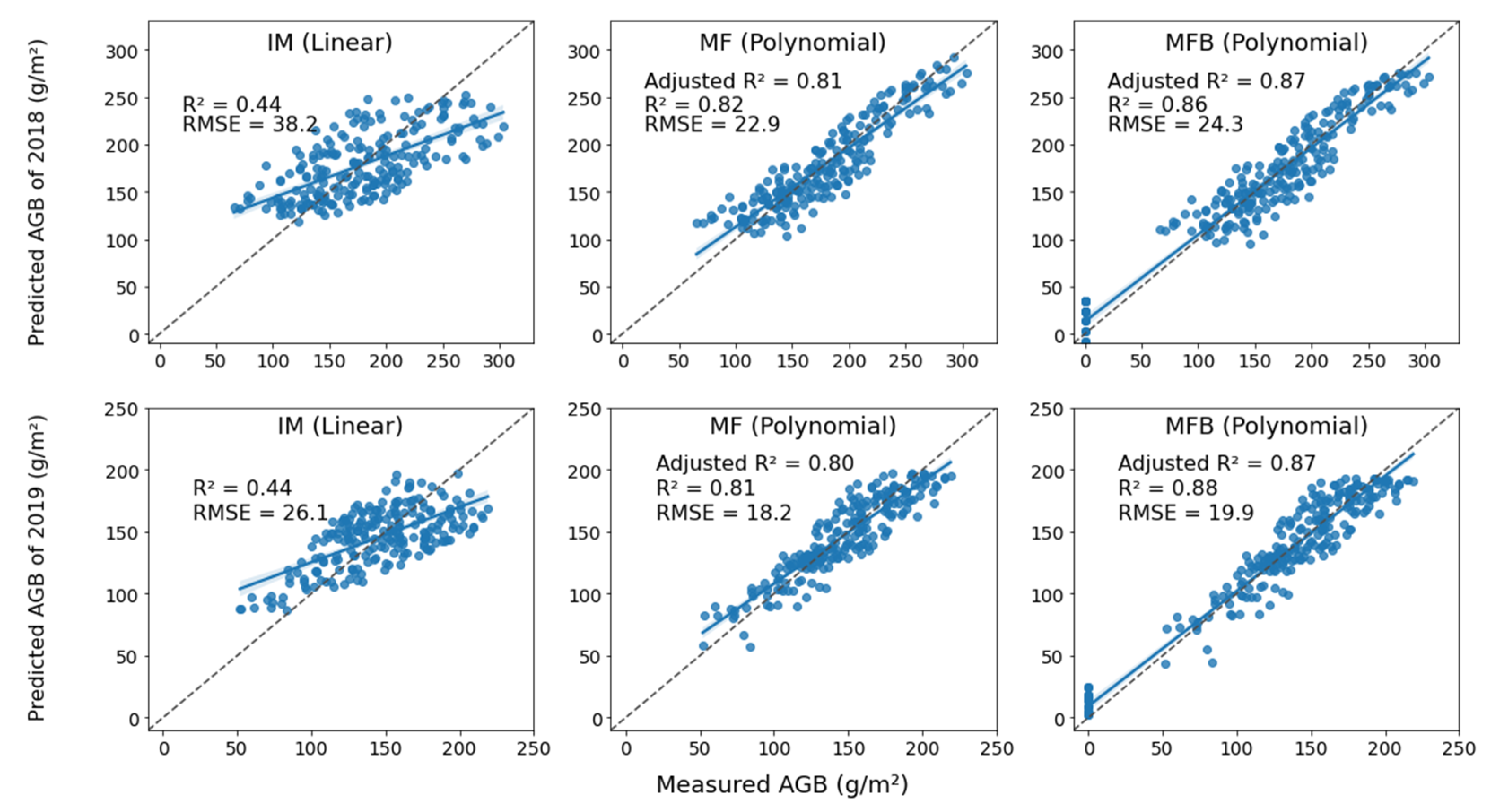
Both linear and polynomial models were evaluated for their accuracy in estimating AGB (Figure 7). The best models were judged from the scatterplots in Figure 8. Generally, the polynomial models outperformed the linear ones except the initial models. Their accuracy in both 2018 and 2019 was rather low (R2 < 0.45). However, model accuracy was highly improved if the model was modified with the mowing factor. Mowing modified models achieved a remarkable accuracy of R2 around 0.70 (linear) and 0.82 (polynomial) in both years. The combination of both mowing and bare ground modifications further improved model accuracy by about 0.04 for 2018 and 0.08 for 2019 (Figure 7). In particular, the polynomial models achieved the highest R2 of 0.86 for 2018, and 0.88 for 2019 (Figure 8). It was worth noting that RMSE increased from 22.9 to 24.3 for 2018 and from 18.2 to 19.9 for 2019 after bare ground metrics were incorporated into the mowing-modified models. However, this metric helped to improve model reliability.

3.3. Effects of Disturbance Severity and Bare Ground on AGB Estimation

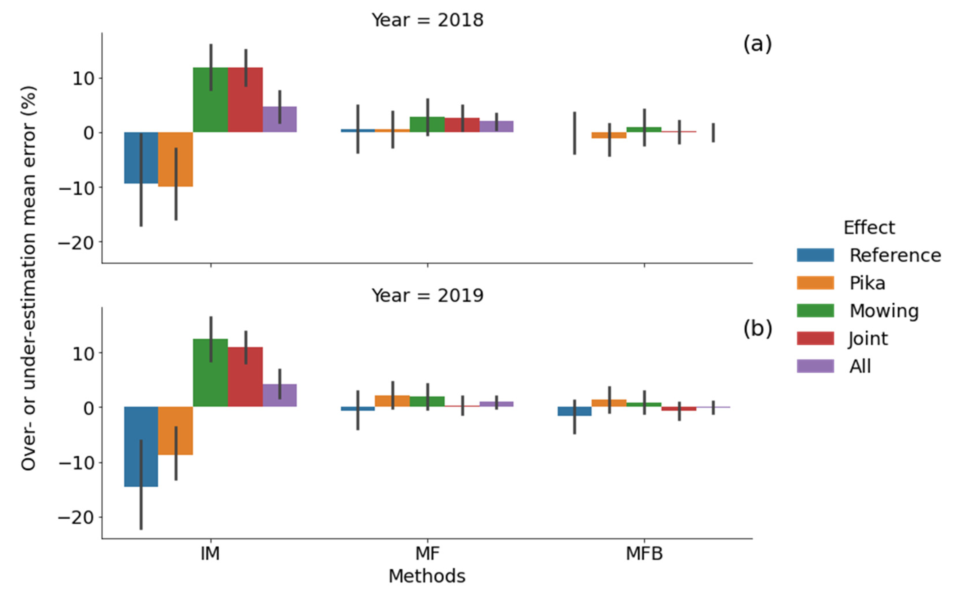
The influence of the severity of sole and joint disturbances on AGB estimation was assessed in terms of mean error (Figure 9). The mowing-modified models underestimated AGB for the non-mowed groups (reference and pika) with an error around −10% in 2018, and a further −15% for the reference group of 2019. The mowed groups (mowing and joint) were all overestimated with an error about 10% in both years. On average, AGB was overestimated by these models with an error around 4.0% in both years. However, if modified by both mowing and bare ground, absolute mean error of estimation was reduced to about 1.0% for the reference groups and less than 3.0% for the other groups in both years. The mean error of all groups was found to be around 2.0% and 1.0% for 2018 and 2019, respectively. Although all the groups had little improvement after both mowing and bare ground modifications in both years, the average mean error of estimation was reduced to close to zero.
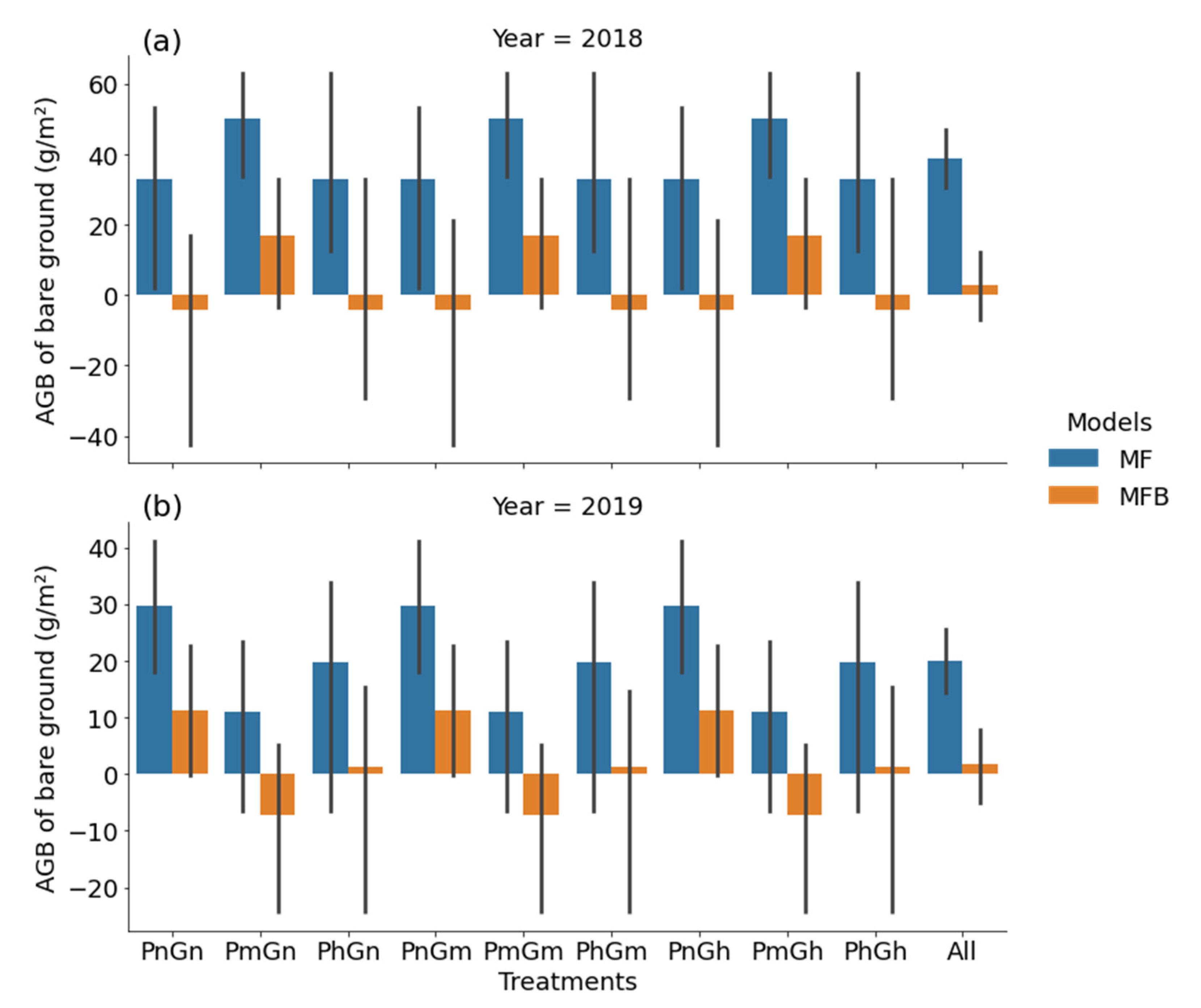
In order to assess the performance of bare ground metrics on improving AGB estimation, the two modified models were compared in terms of the predicted AGB in bare ground areas (Figure 10). The mowing-modified model overestimated bare ground AGB by 32–50 g m−2 for 2018 and 12–30 g m−2 for 2019. This estimation error was effectively reduced to a range from −5 to 18 g m−2 for 2018 and from −8 to 13 g m−2 for 2019 after bare ground metrics were incorporated into the mowing-modified models, although underestimation occurred in some treatments. On average, the consideration of bare ground modification metrics reduced the overestimation from 38 to 4 g m−2 for 2018 and from 19 to 2 g m−2 for 2019. Therefore, both modifications can help to reduce estimation errors caused by the soil background influence.

4. Discussion

4.1. Comparison of Modifications

Of the two modifications, mowing boosted the estimation accuracy to a level similar to that achieved using canopy volume [87,88,89]. However, the estimation accuracy was improved only slightly if the model was further modified by the bare ground metrics, although both modifications jointly improved the estimation accuracy to the highest level possible for both years (Figure 8). Mowing modification was more effective at improving the estimation accuracy than bare ground modification because it was applied universally to the entire experiment plots. In comparison, bare ground was much less extensive spatially in all the plots. It can be predicted that this modification would improve the estimation accuracy more had there been more denudated patches inside the selected experiment plots. Furthermore, after these modifications, the best estimation model changed its nature from linear to polynomial. This change is explained by the pyramidal distribution of grassland biomass vertically [90].
In this study, grazing was simulated via mowing. Studies elsewhere have shown that livestock grazing generally influences grassland AGB differently from artificial grazing simulated via mowing, but the differences are rather small [91]. Grazing effectively influences the vertical structure of biomass by removing biomass equivalently and producing a uniform, smooth horizontal biomass distribution [92]. In comparison, livestock preferentially graze palatable species [93], resulting in an uneven height of plants, while mowing always leads to a uniform height of plants, at least immediately following the mowing. This equivalent height of mowed plants is conducive to achieving a higher AGB estimation accuracy. For instance, the mowed plots had an R2 over 0.70, slightly higher than that of the reference plots (Figure 6), because the latter had an uneven plant height due to natural growth. Grass height affects the accuracy of biomass estimation [94]. The lack of consideration of vegetation height caused high AGB to be underestimated but low AGB to be overestimated by the initial models (Figure 8). Such inaccurate estimations are attributed to the fact that the RGBVI derived from the drone images can only show the aerial view of the grass from above [95].

4.2. Implications

The achievement of a high estimation accuracy requires substantial training samples representative of all the variable vegetation characteristics [96]. An inspection reveals huge differences in RGBVI between the sampled and bare ground areas. Thus, the use of the AGB samples collected from the experimental site may not be sufficiently representative to achieve an accuracy higher than 0.88 because of the under-representation of low AGB. The models constructed from these samples typically overestimate AGB, especially in severely disturbed plots (Figure 10). Therefore, there is a need to build bare ground metrics for expanding the training samples to reduce the estimation inaccuracy of bare ground AGB.
This study has demonstrated the feasibility of using local-scale drone images in estimation grassland AGB based on RGBVI at a rather high accuracy. Naturally, the accuracy will be lower (e.g., less than 0.70) if the estimation is implemented on a broad scale due to much wider spatial variability in vegetation conditions [97,98]. The proposed modification method can be easily replicated elsewhere. In the absence of mowing intensity data, the estimation accuracy can still be improved by substituting the mowing intensity by the stocking rate that can be regarded as a proxy for grazing intensity. This substitution is permissible, as grassland AGB bears a strong relationship with stocking rate and grazing intensity (R2 > 0.72) [55,56]. Thus, the proposed modification methods have the potential to improve the AGB estimation accuracy even for livestock grazed grassland. If applied at a broad scale, the estimation of grassland AGB should be achieved from satellite images with near infrared and shortwave infrared bands. Such images enable other VIs to be derived. It will be interesting to investigate whether the same level of improvement in estimation accuracy can be achieved at a broad scale by both modifications.

5. Conclusions

This study proposes an efficient method to improve the accuracy of estimating grassland AGB from high-resolution drone images. The commonly adopted RGBVI estimation models were further modified by grazing (simulated via mowing) intensity and the quantity of bare ground mapped from the UAV images using support vector machine. Without such modifications, the estimation was achieved at a rather low accuracy (R2 around 0.44) due to overestimation of low AGB values but underestimation of high AGB values, both by the same amount of 10%. However, the estimation accuracy was significantly improved to 0.81 after the model was modified by the mowing intensity that was considered as the proxy for the quantity of biomass on the ground. Nevertheless, further modification by the amount of bare ground improved the estimation only marginally (by 0.04 up to 0.08) to 0.88, an accuracy comparable to that achieved at a broad scale. The proposed mowing modification is more effective than bare ground modification in improving estimation accuracy, as it was applied universally to the entire experimental plots and is able to take into account the vertical structure of grasses, a key indicator of biomass in this instance. In comparison, bare grounds were of limited spatial presence in the study area. Since this modification markedly reduced the overestimation of low AGB values, it can be anticipated that the estimation accuracy would have been improved much more if there had been more bare ground enclosed in the experimental plots. The proposed methods can be used to assess the grassland carrying capacity quickly, thereby supporting more systematic and precise determination of the impacts of stocking rates and grazing practices.

Author Contributions

Experiment design, X.L.; field data collection, J.L.; methodology, Y.S. and J.G.; software, Y.S.; data analysis, Y.S. and J.G.; supervision, J.G.; writing—original draft preparation, Y.S. and J.G.; writing—review and editing, D.M.G.d.T. and G.J.B.; funding acquisition, X.L. All authors have read and agreed to the published version of the manuscript.

Funding

This study was financially supported by a research grant (31872999) from the National Natural Science Foundation of China, Project of the Science and Technology Department of Qinghai Province (2020-ZJ-904), Discipline Innovation and Introducing Talents Program of Higher Education Institutions (the 111 Project, D18013) and Joint Research Project of Three-River- Resource National Park funded by Chinese Academy of Sciences and Qinghai Provincial People’s Government (LHZX-2020-08). Authors gratefully acknowledge support from the University of Auckland as part of the Three Brothers Collaboration Project.

Institutional Review Board Statement

Not applicable.

Informed Consent Statement

Not applicable.

Data Availability Statement

No new data were created or analyzed in this study. Data sharing is not applicable to this article.

Conflicts of Interest

The authors declare no conflict of interest.

References

  1. Chen, Z.X.; Zhang, X.S. Value of ecosystem services in China. Chin. Sci. Bull. 2000, 45, 870–876. [Google Scholar] [CrossRef]
  2. Li, X.L.; Gao, J.; Brierley, G.; Qiao, Y.M.; Zhang, J.; Yang, Y.W. Rangeland Degradation on the Qinghai-Tibet Plateau: Implications for Rehabilitation. Land Degrad. Dev. 2013, 24, 72–80. [Google Scholar] [CrossRef]
  3. Dong, S.K.; Shang, Z.H.; Gao, J.X.; Boone, R.B. Enhancing sustainability of grassland ecosystems through ecological restoration and grazing management in an era of climate change on Qinghai-Tibetan Plateau. Agric. Ecosyst. Environ. 2020, 287. [Google Scholar] [CrossRef]
  4. Yu, C.; Zhang, J.; Pang, X.P.; Wang, Q.; Zhou, Y.P.; Guo, Z.G. Soil disturbance and disturbance intensity: Response of soil nutrient concentrations of alpine meadow to plateau pika bioturbation in the Qinghai-Tibetan Plateau, China. Geoderma 2017, 307, 98–106. [Google Scholar] [CrossRef]
  5. Gao, Q.; Guo, Y.; Xu, H.; Ganjurjav, H.; Li, Y.; Wan, Y.; Qin, X.; Ma, X.; Liu, S. Climate change and its impacts on vegetation distribution and net primary productivity of the alpine ecosystem in the Qinghai-Tibetan Plateau. Sci. Total Environ. 2016, 554-555, 34–41. [Google Scholar] [CrossRef]
  6. Liu, J.; Xu, X.; Shao, Q. Grassland degradation in the “Three-River Headwaters” region, Qinghai Province. J. Geogr. Sci. 2008, 18, 259–273. [Google Scholar] [CrossRef]
  7. Li, X.L.; Perry, L.W.G.; Brierley, G.; Gao, J.; Zhang, J.; Yang, Y.W. Restoration prospects for Heitutan degraded grassland in the Sanjiangyuan. J. Mt. Sci. Engl. 2013, 10, 687–698. [Google Scholar] [CrossRef] [Green Version]
  8. Li, L.; Zhang, Y.; Wu, J.; Li, S.; Zhang, B.; Zu, J.; Zhang, H.; Ding, M.; Paudel, B. Increasing sensitivity of alpine grasslands to climate variability along an elevational gradient on the Qinghai-Tibet Plateau. Sci. Total Environ. 2019, 678, 21–29. [Google Scholar] [CrossRef] [PubMed]
  9. Zhang, R.Y.; Wang, Z.W.; Han, G.D.; Schellenberg, M.P.; Wu, Q.; Gu, C. Grazing induced changes in plant diversity is a critical factor controlling grassland productivity in the Desert Steppe, Northern China. Agric. Ecosyst. Environ. 2018, 265, 73–83. [Google Scholar] [CrossRef]
  10. Huang, W.; Bruemmer, B.; Huntsinger, L. Incorporating measures of grassland productivity into efficiency estimates for livestock grazing on the Qinghai-Tibetan Plateau in China. Ecol. Econ. 2016, 122, 1–11. [Google Scholar] [CrossRef]
  11. Zhang, Y.; Zhang, C.; Wang, Z.; Chen, Y.; Gang, C.; An, R.; Li, J. Vegetation dynamics and its driving forces from climate change and human activities in the Three-River Source Region, China from 1982 to 2012. Sci. Total Environ. 2016, 563-564, 210–220. [Google Scholar] [CrossRef]
  12. Liu, Y.; Wang, Q.; Zhang, Z.; Tong, L.; Wang, Z.; Li, J. Grassland dynamics in responses to climate variation and human activities in China from 2000 to 2013. Sci. Total Environ. 2019, 690, 27–39. [Google Scholar] [CrossRef]
  13. Chen, B.X.; Zhang, X.Z.; Tao, J.; Wu, J.S.; Wang, J.S.; Shi, P.L.; Zhang, Y.J.; Yu, C.Q. The impact of climate change and anthropogenic activities on alpine grassland over the Qinghai-Tibet Plateau. Agric. For. Meteorol. 2014, 189, 11–18. [Google Scholar] [CrossRef]
  14. Gang, C.C.; Zhou, W.; Chen, Y.Z.; Wang, Z.Q.; Sun, Z.G.; Li, J.L.; Qi, J.G.; Odeh, I. Quantitative assessment of the contributions of climate change and human activities on global grassland degradation. Environ. Earth Sci. 2014, 72, 4273–4282. [Google Scholar] [CrossRef]
  15. Huang, K.; Zhang, Y.J.; Zhu, J.T.; Liu, Y.J.; Zu, J.X.; Zhang, J. The Influences of Climate Change and Human Activities on Vegetation Dynamics in the Qinghai-Tibet Plateau. Remote Sens. 2016, 8, 876. [Google Scholar] [CrossRef] [Green Version]
  16. Zhou, W.; Gang, C.C.; Zhou, L.; Chen, Y.Z.; Li, J.L.; Ju, W.M.; Odeh, I. Dynamic of grassland vegetation degradation and its quantitative assessment in the northwest China. Acta Oecol. 2014, 55, 86–96. [Google Scholar] [CrossRef]
  17. Liu, Y.Y.; Zhang, Z.Y.; Tong, L.J.; Khalifa, M.; Wang, Q.; Gang, C.C.; Wang, Z.Q.; Li, J.L.; Sun, Z.G. Assessing the effects of climate variation and human activities on grassland degradation and restoration across the globe. Ecol. Indic. 2019, 106, 105504. [Google Scholar] [CrossRef]
  18. Cao, F.F.; Li, J.X.; Fu, X.; Wu, G. Impacts of land conversion and management measures on net primary productivity in semi-arid grassland. Ecosyst. Health Sustain. 2020, 6, 1749010. [Google Scholar] [CrossRef] [Green Version]
  19. Yao, X.X.; Wu, J.P.; Gong, X.Y.; Lang, X.; Wang, C.L.; Song, S.Z.; Ahmad, A.A. Effects of long term fencing on biomass, coverage, density, biodiversity and nutritional values of vegetation community in an alpine meadow of the Qinghai-Tibet Plateau. Ecol. Eng. 2019, 130, 80–93. [Google Scholar] [CrossRef]
  20. Klaus, V.H.; Boch, S.; Boeddinghaus, R.S.; Holzel, N.; Kandeler, E.; Marhan, S.; Oelmann, Y.; Prati, D.; Regan, K.M.; Schmitt, B.; et al. Temporal and small-scale spatial variation in grassland productivity, biomass quality, and nutrient limitation. Plant Ecol. 2016, 217, 843–856. [Google Scholar] [CrossRef]
  21. Wang, Z.; Zhang, Y.; Yang, Y.; Zhou, W.; Gang, C.; Zhang, Y.; Li, J.; An, R.; Wang, K.; Odeh, I.; et al. Quantitative assess the driving forces on the grassland degradation in the Qinghai–Tibet Plateau, in China. Ecol. Inform. 2016, 33, 32–44. [Google Scholar] [CrossRef]
  22. Zhang, Y.; Wang, Q.; Wang, Z.; Yang, Y.; Li, J. Impact of human activities and climate change on the grassland dynamics under different regime policies in the Mongolian Plateau. Sci. Total Environ. 2020, 698, 134304. [Google Scholar] [CrossRef]
  23. Liang, T.G.; Yang, S.X.; Feng, Q.S.; Liu, B.K.; Zhang, R.P.; Huang, X.D.; Xie, H.J. Multi-factor modeling of above-ground biomass in alpine grassland: A case study in the Three-River Headwaters Region, China. Remote Sens. Environ. 2016, 186, 164–172. [Google Scholar] [CrossRef]
  24. Sun, Q.L.; Li, B.L.; Zhang, T.; Yuan, Y.C.; Gao, X.Z.; Ge, J.S.; Li, F.; Zhang, Z.J. An improved Biome-BGC model for estimating net primary productivity of alpine meadow on the Qinghai-Tibet Plateau. Ecol. Model. 2017, 350, 55–68. [Google Scholar] [CrossRef]
  25. Wang, S.Y.; Zhang, B.; Yang, Q.C.; Chen, G.S.; Yang, B.J.; Lu, L.L.; Shen, M.; Peng, Y.Y. Responses of net primary productivity to phenological dynamics in the Tibetan Plateau, China. Agric. For. Meteorol. 2017, 232, 235–246. [Google Scholar] [CrossRef]
  26. Shen, M.; Tang, Y.; Klein, J.; Zhang, P.; Gu, S.; Shimono, A.; Chen, J. Estimation of aboveground biomass using in situ hyperspectral measurements in five major grassland ecosystems on the Tibetan Plateau. J. Plant Ecol. 2008, 1, 247–257. [Google Scholar] [CrossRef] [Green Version]
  27. Han, D.M.; Wang, G.Q.; Xue, B.L.; Liu, T.X.; Yinglan, A.; Xu, X.Y. Evaluation of semiarid grassland degradation in North China from multiple perspectives. Ecol. Eng. 2018, 112, 41–50. [Google Scholar] [CrossRef]
  28. Sun, F.D.; Chen, W.Y.; Liu, L.; Liu, W.; Cai, Y.M.; Smith, P. Effects of plateau pika activities on seasonal plant biomass and soil properties in the alpine meadow ecosystems of the Tibetan Plateau. Grassl. Sci. 2015, 61, 195–203. [Google Scholar] [CrossRef]
  29. Waite, R.B. The Application of Visual Estimation Procedures for Monitoring Pasture Yield and Composition in Exclosures and Small Plots. Trop. Grassl. 1994, 28, 38–42. [Google Scholar]
  30. Catchpole, W.R.; Wheeler, C.J. Estimating Plant Biomass—A Review of Techniques. Aust. J. Ecol. 1992, 17, 121–131. [Google Scholar] [CrossRef]
  31. Xu, B.; Yang, X.C.; Tao, W.G.; Qin, Z.H.; Liu, H.Q.; Miao, J.M.; Bi, Y.Y. MODIS-based remote sensing monitoring of grass production in China. Int. J. Remote Sens. 2008, 29, 5313–5327. [Google Scholar] [CrossRef]
  32. Anaya, J.A.; Chuvieco, E.; Palacios-Orueta, A. Aboveground biomass assessment in Colombia: A remote sensing approach. For. Ecol. Manag. 2009, 257, 1237–1246. [Google Scholar] [CrossRef]
  33. Todd, S.W.; Hoffer, R.M.; Milchunas, D.G. Biomass estimation on grazed and ungrazed rangelands using spectral indices. Int. J. Remote Sens. 1998, 19, 427–438. [Google Scholar] [CrossRef]
  34. Gamon, J.A.; Field, C.B.; Goulden, M.L.; Griffin, K.L.; Hartley, A.E.; Joel, G.; Penuelas, J.; Valentini, R. Relationships between NDVI, canopy structure, and photosynthesis in three Californian vegetation types. Ecol. Appl. 1995, 5, 28–41. [Google Scholar] [CrossRef] [Green Version]
  35. Liu, Y.; Zha, Y.; Gao, J.; Ni, S. Assessment of grassland degradation near Lake Qinghai, West China, using Landsat TM and in situ reflectance spectra data. Int. J. Remote Sens. 2004, 25, 4177–4189. [Google Scholar] [CrossRef]
  36. Marsett, R.C.; Qi, J.G.; Heilman, P.; Biedenbender, S.H.; Watson, M.C.; Amer, S.; Weltz, M.; Goodrich, D.; Marsett, R. Remote sensing for grassland management in the arid Southwest. Rangel. Ecol. Manag. 2006, 59, 530–540. [Google Scholar] [CrossRef]
  37. Zhu, L. Remote Sensing Based Vegetation Dynamics in Southern Africa: Physiographic Gradients Determine the Relative Importance of Environmental Controls on Savanna Vegetation. Ph.D. Thesis, University of Florida, Ann Arbor, MI, USA, 2014. [Google Scholar]
  38. Tucker, C.J.; Sellers, P.J. Satellite Remote-Sensing of Primary Production. Int. J. Remote Sens. 1986, 7, 1395–1416. [Google Scholar] [CrossRef]
  39. Bannari, A.; Morin, D.; Bonn, F.; Huete, A.R. A review of vegetation indices. Remote Sens. Rev. 1995, 13, 95–120. [Google Scholar] [CrossRef]
  40. Lussem, U.; Bolten, A.; Gnyp, M.; Jasper, J.; Bareth, G. Evaluation of RGB-based vegetation indices from UAV imagery to estimate forage yield in grassland. ISPRS Int. Arch. Photogramm. Remote Sens. Spat. Inf. Sci. 2018, 42, 1215–1219. [Google Scholar] [CrossRef] [Green Version]
  41. Torres-Sánchez, J.; Peña, J.M.; de Castro, A.I.; López-Granados, F. Multi-temporal mapping of the vegetation fraction in early-season wheat fields using images from UAV. Comput. Electron. Agric. 2014, 103, 104–113. [Google Scholar] [CrossRef]
  42. Berni, J.; Zarco-Tejada, P.; Suárez, L.; González-Dugo, V.; Fereres, E. Remote sensing of vegetation from UAV platforms using lightweight multispectral and thermal imaging sensors. Int. Arch. Photogramm. Remote Sens. Spat. Inf. Sci. 2009, 38, 6. [Google Scholar]
  43. Themistocleous, K. The use of UAVs for monitoring land degradation. In Proceedings of the Earth Resources and Environmental Remote Sensing/GIS Applications VIII, Warsaw, Poland, 11–14 September 2017; p. 104280E. [Google Scholar]
  44. Candiago, S.; Remondino, F.; De Giglio, M.; Dubbini, M.; Gattelli, M. Evaluating multispectral images and vegetation indices for precision farming applications from UAV images. Remote Sens. 2015, 7, 4026–4047. [Google Scholar] [CrossRef] [Green Version]
  45. Chen, J.; Yi, S.; Qin, Y.; Wang, X. Improving estimates of fractional vegetation cover based on UAV in alpine grassland on the Qinghai–Tibetan Plateau. Int. J. Remote Sens. 2016, 37, 1922–1936. [Google Scholar] [CrossRef]
  46. Zhao, F.; Xu, B.; Yang, X.; Jin, Y.; Li, J.; Xia, L.; Chen, S.; Ma, H. Remote sensing estimates of grassland aboveground biomass based on MODIS Net Primary Productivity (NPP): A case study in the Xilingol grassland of northern China. Remote Sens. 2014, 6, 5368–5386. [Google Scholar] [CrossRef] [Green Version]
  47. Zhang, R.; Zhou, Y.; Luo, H.; Wang, F.; Wang, S. Estimation and analysis of spatiotemporal dynamics of the net primary productivity integrating efficiency model with process model in karst area. Remote Sens. 2017, 9, 477. [Google Scholar] [CrossRef] [Green Version]
  48. Greaves, H.E.; Vierling, L.A.; Eitel, J.U.H.; Boelman, N.T.; Magney, T.S.; Prager, C.M.; Griffin, K.L. Estimating aboveground biomass and leaf area of low-stature Arctic shrubs with terrestrial LiDAR. Remote Sens. Environ. 2015, 164, 26–35. [Google Scholar] [CrossRef]
  49. Jayathunga, S.; Owari, T.; Tsuyuki, S. Evaluating the performance of photogrammetric products using fixed-wing UAV imagery over a mixed conifer-broadleaf forest: Comparison with airborne laser scanning. Remote Sens. 2018, 10, 187. [Google Scholar] [CrossRef] [Green Version]
  50. Dandois, J.P.; Ellis, E.C. High spatial resolution three-dimensional mapping of vegetation spectral dynamics using computer vision. Remote Sens. Environ. 2013, 136, 259–276. [Google Scholar] [CrossRef] [Green Version]
  51. Kalacska, M.; Chmura, G.L.; Lucanus, O.; Bérubé, D.; Arroyo-Mora, J.P. Structure from motion will revolutionize analyses of tidal wetland landscapes. Remote Sens. Environ. 2017, 199, 14–24. [Google Scholar] [CrossRef]
  52. Schulze-Brüninghoff, D.; Hensgen, F.; Wachendorf, M.; Astor, T. Methods for LiDAR-based estimation of extensive grassland biomass. Comput. Electron. Agric. 2019, 156, 693–699. [Google Scholar] [CrossRef]
  53. Xu, K.; Su, Y.; Liu, J.; Hu, T.; Jin, S.; Ma, Q.; Zhai, Q.; Wang, R.; Zhang, J.; Li, Y.; et al. Estimation of degraded grassland aboveground biomass using machine learning methods from terrestrial laser scanning data. Ecol. Indic. 2020, 108, 105747. [Google Scholar] [CrossRef]
  54. Wijesingha, J.; Moeckel, T.; Hensgen, F.; Wachendorf, M. Evaluation of 3D point cloud-based models for the prediction of grassland biomass. Int. J. Appl. Earth Obs. Geoinf. 2019, 78, 352–359. [Google Scholar] [CrossRef]
  55. Numata, I.; Roberts, D.A.; Chadwick, O.A.; Schimel, J.; Sampaio, F.R.; Leonidas, F.C.; Soares, J.V. Characterization of pasture biophysical properties and the impact of grazing intensity using remotely sensed data. Remote Sens. Environ. 2007, 109, 314–327. [Google Scholar] [CrossRef]
  56. Deng, L.; Sweeney, S.; Shangguan, Z.P. Grassland responses to grazing disturbance: Plant diversity changes with grazing intensity in a desert steppe. Grass Forage Sci. 2014, 69, 524–533. [Google Scholar] [CrossRef]
  57. Isselstein, J.; Griffith, B.A.; Pradel, P.; Venerus, S. Effects of livestock breed and grazing intensity on biodiversity and production in grazing systems. 1. Nutritive value of herbage and livestock performance. Grass Forage Sci. 2007, 62, 145–158. [Google Scholar] [CrossRef]
  58. Zhang, Y.; Dong, S.; Gao, Q.; Liu, S.; Liang, Y.; Cao, X. Responses of alpine vegetation and soils to the disturbance of plateau pika ( Ochotona curzoniae ) at burrow level on the Qinghai–Tibetan Plateau of China. Ecol. Eng. 2016, 88, 232–236. [Google Scholar] [CrossRef]
  59. Chen, J.J.; Yi, S.H.; Qin, Y. The contribution of plateau pika disturbance and erosion on patchy alpine grassland soil on the Qinghai-Tibetan Plateau: Implications for grassland restoration. Geoderma 2017, 297, 1–9. [Google Scholar] [CrossRef]
  60. Tang, Z.; Zhang, Y.; Cong, N.; Wimberly, M.; Wang, L.; Huang, K.; Li, J.; Zu, J.; Zhu, Y.; Chen, N. Spatial pattern of pika holes and their effects on vegetation coverage on the Tibetan Plateau: An analysis using unmanned aerial vehicle imagery. Ecol. Indic. 2019, 107, 105551. [Google Scholar] [CrossRef]
  61. Ren, H.; Zhou, G.; Zhang, F. Using negative soil adjustment factor in soil-adjusted vegetation index (SAVI) for aboveground living biomass estimation in arid grasslands. Remote Sens. Environ. 2018, 209, 439–445. [Google Scholar] [CrossRef]
  62. Xue, J.R.; Su, B.F. Significant Remote Sensing Vegetation Indices: A Review of Developments and Applications. J. Sens. 2017, 2017, 1353691. [Google Scholar] [CrossRef] [Green Version]
  63. Huete, A.R. A soil-adjusted vegetation index (SAVI). Remote Sens. Environ. 1988, 25, 295–309. [Google Scholar] [CrossRef]
  64. Du, J.; Yi, S.; Qin, Y.; Yu, H.; Ma, J. Distribution and cause of plateau pika(Ochotona curzoniae) burrows in Henan Mongolian Autonomous county, Qinghai Province. J. Anhui Agric. Univ. 2019, 43, 415–419. [Google Scholar] [CrossRef]
  65. Zhang, Y.; Fan, J.; Zhang, H. A method for calculating the suitable monthly carrying capacity of seasonal pasture-Taking heriheng Village, Henan County, Qinghai Province as example. Pratacult. Sci. 2018, 35, 1308–1314. [Google Scholar]
  66. Wei, X.; Li, S.; Yang, P.; Cheng, H. Soil erosion and vegetation succession in alpine Kobresia steppe meadow caused by plateau pika—A case study of Nagqu County, Tibet. Chin. Geogr. Sci. 2007, 17, 75–81. [Google Scholar] [CrossRef] [Green Version]
  67. Xiao, Y.; Liang, J.; Sha, Q. The distribution of the plateau pika and its effect on grass Kobresia pygmaea in the Tianjun and Kangyang regions. Contrib. Rodent Control Rodent Biol. Beijing Sci. Press 1981, 4, 114–124. [Google Scholar]
  68. Hoffmann, R.S.; Lunde, D.; MacKinnon, J.; Wilson, D.E.; Wozencraft, W.C.; Gemma, F. Mammals of China; Princeton University Press: Princeton, NJ, USA, 2013. [Google Scholar]
  69. Pang, X.P.; Guo, Z.G. Plateau pika disturbances alter plant productivity and soil nutrients in alpine meadows of the Qinghai-Tibetan Plateau, China. Rangel. J. 2017, 39, 133–144. [Google Scholar] [CrossRef]
  70. Sun, F.; Long, R.; Lu, C. Effects of rodent activities on primary productivity and soil physical characteristics in alpine meadow. Res. Soil Water Conserv. 2009, 16, 225–229. [Google Scholar]
  71. Han, T.; Hua, L.; Xu, G. Rodent damage assessment on the plateau pika. Acta Pratacult. Sin. 2008, 17, 130–137. [Google Scholar] [CrossRef]
  72. Sun, F. Effects of Burrowing Plateau Pika (Ochotona Curzoniae) Densities on Primary Productivity and Soil Resource Characteristics in Alpine Meadow. Ph.D. Thesis, Gansu Agricultural University, Lanzhou, China, 2008. [Google Scholar]
  73. Dobson, F.S.; Smith, A.T.; Gao, W.X. Social and ecological influences on dispersal and philopatry in the plateau pika (Ochotona curzoniae). Behav. Ecol. 1998, 9, 622–635. [Google Scholar] [CrossRef] [Green Version]
  74. Jerrentrup, J.S.; Wrage-Mönnig, N.; Röver, K.U.; Isselstein, J. Grazing intensity affects insect diversity via sward structure and heterogeneity in a long-term experiment. J. Appl. Ecol. 2014, 51, 968–977. [Google Scholar] [CrossRef]
  75. Law, Q.D.; Bigelow, C.A.; Patton, A.J. Selecting Turfgrasses and Mowing Practices that Reduce Mowing Requirements. Crop. Sci. 2016, 56, 3318–3327. [Google Scholar] [CrossRef] [Green Version]
  76. De Carvalho, O.A.; Guimarães, R.F.; Silva, N.C.; Gillespie, A.R.; Gomes, R.A.T.; Silva, C.R.; De Carvalho, A.P.F. Radiometric normalization of temporal images combining automatic detection of pseudo-invariant features from the distance and similarity spectral measures, density scatterplot analysis, and robust regression. Remote Sens. 2013, 5, 2763–2794. [Google Scholar] [CrossRef] [Green Version]
  77. Bareth, G.; Bolten, A.; Hollberg, J.; Aasen, H.; Burkart, A.; Schellberg, J. Feasibility study of using non-calibrated UAV-based RGB imagery for grassland monitoring: Case study at the Rengen Long-term Grassland Experiment (RGE), Germany. DGPF Tag. 2015, 24, 1–7. [Google Scholar]
  78. Wang, L. Support Vector Machines: Theory and Applications; Springer Science & Business Media: New York, NY, USA, 2005; Volume 177. [Google Scholar]
  79. Kruse, F.A.; Lefkoff, A.B.; Boardman, J.W.; Heidebrecht, K.B.; Shapiro, A.T.; Barloon, P.J.; Goetz, A.F.H. The spectral image processing system (SIPS)—interactive visualization and analysis of imaging spectrometer data. Remote Sens. Environ. 1993, 44, 145–163. [Google Scholar] [CrossRef]
  80. Congalton, R.G. A Review of Assessing the Accuracy of Classifications of Remotely Sensed Data. Remote Sens. Environ. 1991, 37, 35–46. [Google Scholar] [CrossRef]
  81. Stehman, S.V. Estimating the kappa coefficient and its variance under stratified random sampling. Photogramm. Eng. Remote Sens. 1996, 62, 401–407. [Google Scholar]
  82. Bendig, J.; Yu, K.; Aasen, H.; Bolten, A.; Bennertz, S.; Broscheit, J.; Gnyp, M.L.; Bareth, G. Combining UAV-based plant height from crop surface models, visible, and near infrared vegetation indices for biomass monitoring in barley. Int. J. Appl. Earth Obs. Geoinf. 2015, 39, 79–87. [Google Scholar] [CrossRef]
  83. Zheng, H.; Cheng, T.; Zhou, M.; Li, D.; Yao, X.; Tian, Y.; Cao, W.; Zhu, Y. Improved estimation of rice aboveground biomass combining textural and spectral analysis of UAV imagery. Precis. Agric. 2019, 20, 611–629. [Google Scholar] [CrossRef]
  84. Lu, N.; Zhou, J.; Han, Z.; Li, D.; Cao, Q.; Yao, X.; Tian, Y.; Zhu, Y.; Cao, W.; Cheng, T. Improved estimation of aboveground biomass in wheat from RGB imagery and point cloud data acquired with a low-cost unmanned aerial vehicle system. Plant Methods 2019, 15, 17. [Google Scholar] [CrossRef] [PubMed] [Green Version]
  85. Zhu, J.; Huang, Z.H.; Sun, H.; Wang, G.X. Mapping Forest Ecosystem Biomass Density for Xiangjiang River Basin by Combining Plot and Remote Sensing Data and Comparing Spatial Extrapolation Methods. Remote Sens. 2017, 9, 241. [Google Scholar] [CrossRef] [Green Version]
  86. Wang, C.; Nie, S.; Xi, X.; Luo, S.; Sun, X. Estimating the biomass of maize with hyperspectral and LiDAR data. Remote Sens. 2017, 9, 11. [Google Scholar] [CrossRef] [Green Version]
  87. Greaves, H.E.; Vierling, L.A.; Eitel, J.U.H.; Boelman, N.T.; Magney, T.S.; Prager, C.M.; Griffin, K.L. High-resolution mapping of aboveground shrub biomass in Arctic tundra using airborne lidar and imagery. Remote Sens. Environ. 2016, 184, 361–373. [Google Scholar] [CrossRef]
  88. Zolkos, S.G.; Goetz, S.J.; Dubayah, R. A meta-analysis of terrestrial aboveground biomass estimation using lidar remote sensing. Remote Sens. Environ. 2013, 128, 289–298. [Google Scholar] [CrossRef]
  89. Borra-Serrano, I.; De Swaef, T.; Muylle, H.; Nuyttens, D.; Vangeyte, J.; Mertens, K.; Saeys, W.; Somers, B.; Roldan-Ruiz, I.; Lootens, P. Canopy height measurements and non-destructive biomass estimation of Lolium perenne swards using UAV imagery. Grass Forage Sci. 2019, 74, 356–369. [Google Scholar] [CrossRef]
  90. Tackenberg, O. A new method for non-destructive measurement of biomass, growth rates, vertical biomass distribution and dry matter content based on digital image analysis. Ann. Bot. 2007, 99, 777–783. [Google Scholar] [CrossRef] [PubMed]
  91. Talle, M.; Deak, B.; Poschlod, P.; Valko, O.; Westerberg, L.; Milberg, P. Grazing vs. mowing: A meta-analysis of biodiversity benefits for grassland management. Agric. Ecosyst. Environ. 2016, 222, 200–212. [Google Scholar] [CrossRef]
  92. Milchunas, D.; Lauenroth, W. Three-dimensional distribution of plant biomass in relation to grazing and topography in the shortgrass steppe. Oikos 1989, 55, 82–86. [Google Scholar] [CrossRef]
  93. Cao, J.; Holden, N.M.; Lü, X.T.; Du, G. The effect of grazing management on plant species richness on the Qinghai-Tibetan Plateau. Grass Forage Sci. 2011, 66, 333–336. [Google Scholar] [CrossRef]
  94. Han, L.; Yang, G.J.; Dai, H.Y.; Xu, B.; Yang, H.; Feng, H.K.; Li, Z.H.; Yang, X.D. Modeling maize above-ground biomass based on machine learning approaches using UAV remote-sensing data. Plant Methods 2019, 15, 10. [Google Scholar] [CrossRef] [PubMed] [Green Version]
  95. Selkowitz, D.J. A comparison of multi-spectral, multi-angular, and multi-temporal remote sensing datasets for fractional shrub canopy mapping in Arctic Alaska. Remote Sens. Environ. 2010, 114, 1338–1352. [Google Scholar] [CrossRef]
  96. Heckmann, T.; Gegg, K.; Gegg, A.; Becht, M. Sample size matters: Investigating the effect of sample size on a logistic regression susceptibility model for debris flows. Nat. Hazards Earth Syst. Sci. 2014, 14, 259. [Google Scholar] [CrossRef] [Green Version]
  97. Guerini Filho, M.; Kuplich, T.M.; Quadros, F.L.F.D. Estimating natural grassland biomass by vegetation indices using Sentinel 2 remote sensing data. Int. J. Remote Sens 2019, 41, 2861–2876. [Google Scholar] [CrossRef]
  98. Quan, X.W.; He, B.B.; Yebra, M.; Yin, C.M.; Liao, Z.M.; Zhang, X.T.; Li, X. A radiative transfer model-based method for the estimation of grassland aboveground biomass. Int. J. Appl. Earth Obs. Geoinf. 2017, 54, 159–168. [Google Scholar] [CrossRef]
Figure 1. Location of the study site and the experiment settings (1, 2, 3 represent three replications of the same treatment).
Remotesensing 13 02105 g001
Figure 2. Images of the study site showing the experimental area with its weather station (a) and the above/below ground characteristics of the plot fencing (b).
Remotesensing 13 02105 g002
Figure 3. The work flow of the proposed models (IM is the initial model, MF is the mowing ratio modified model, MFB is the model modified by both mowing ratio and bare ground metrics).
Remotesensing 13 02105 g003
Figure 4. The mowing intensity modification ratio (F): (a) the year of 2018; (b) the year of 2019.
Remotesensing 13 02105 g004
Figure 5. RGBVI value of sampled quarter and extracted bare ground: (a) the year of 2018; (b) the year of 2019.
Remotesensing 13 02105 g005
Figure 6. Linear regression relationship between RGBVI and in situ measured AGB by effect severity: (a) regression models by mowing severity in 2018; (b) regression models by pika severity in 2018; (c) regression models by mowing severity in 2019; (d) regression models by pika severity in 2019.
Remotesensing 13 02105 g006
Figure 7. Modelling accuracy comparison before and after modifications (IM is the initial model, MF is the mowing ratio modified model, MFB is the model modified by both mowing ratio and bare ground metrics): (a) modeling accuracy comparison in 2018; (b) modeling accuracy comparison in 2019.
Remotesensing 13 02105 g007
Figure 8. Cross validation scatterplots of predicted versus in situ measured AGB (IM is the initial model, MF is the mowing ratio modified model, MFB is the model modified by both mowing ratio and bare ground metrics).
Remotesensing 13 02105 g008
Figure 9. Comparison of over- and under-estimation mean error among the disturbance groups (IM is the initial model, MF is the mowing ratio modified model, MFB is the model modified by both mowing ratio and bare ground metrics): (a) AGB estimation errors in 2018; (b) AGB estimation errors in 2019.
Remotesensing 13 02105 g009
Figure 10. The over- or under-estimation of AGB caused by bare ground (MF is the mowing ratio modified model, MFB is the model modified by both mowing ratio and bare ground metrics): (a) estimation errors of bare ground in 2018; (b) estimation errors of bare ground in 2019.
Remotesensing 13 02105 g010
Table 1. Information about the treatments.
EffectTreatmentDisturbance Severity
PikaMowing
ReferencePnGnNoneNone
PikaPmGnMediumNone
PhGnHighNone
MowingPnGmNoneHigh
PnGhNoneMedium
JointPmGmMediumHigh
PhGmHighHigh
PmGhMediumMedium
PhGhHighMedium
Table 2. The summary of field measured AGB.
TreatmentSeverity2018 AGB (g m−2)2019 AGB (g m−2)
Min.Mean ± SDMax.LSDMin.Mean ± SDMax.LSD
MowingNone108.00200.24 ± 52.00303.20a96.60166.37 ± 30.68219.11a
Medium98.03193.80 ± 42.26273.84a51.98149.90 ± 30.84207.91b
High65.60140.52 ± 34.30218.96b52.96120.65 ± 26.55174.07c
PikaNone77.92188.46 ± 46.59284.96a52.96150.21 ± 30.82206.92a
Medium71.12166.47 ± 48.78279.36a51.98138.78 ± 38.41209.43a
High65.60179.66 ± 54.96303.20a73.39147.93 ± 34.23219.11a
All65.60178.20 ± 51.04303.20 51.98145.64 ± 34.97219.11
SD: standard deviations. LSD: least significant difference (α < 0.05). Lowercase letters (a–c) represent the significant difference in the two treatments separately.
Publisher’s Note: MDPI stays neutral with regard to jurisdictional claims in published maps and institutional affiliations.