Deep Learning for Detection of Visible Land Boundaries from UAV Imagery

Abstract

Current efforts aim to accelerate cadastral mapping through innovative and automated approaches and can be used to both create and update cadastral maps. This research aims to automate the detection of visible land boundaries from unmanned aerial vehicle (UAV) imagery using deep learning. In addition, we wanted to evaluate the advantages and disadvantages of programming-based deep learning compared to commercial software-based deep learning. For the first case, we used the convolutional neural network U-Net, implemented in Keras, written in Python using the TensorFlow library. For commercial software-based deep learning, we used ENVINet5. UAV imageries from different areas were used to train the U-Net model, which was performed in Google Collaboratory and tested in the study area in Odranci, Slovenia. The results were compared with the results of ENVINet5 using the same datasets. The results showed that both models achieved an overall accuracy of over 95%. The high accuracy is due to the problem of unbalanced classes, which is usually present in boundary detection tasks. U-Net provided a recall of 0.35 and a precision of 0.68 when the threshold was set to 0.5. A threshold can be viewed as a tool for filtering predicted boundary maps and balancing recall and precision. For equitable comparison with ENVINet5, the threshold was increased. U-Net provided more balanced results, a recall of 0.65 and a precision of 0.41, compared to ENVINet5 recall of 0.84 and a precision of 0.35. Programming-based deep learning provides a more flexible yet complex approach to boundary mapping than software-based, which is rigid and does not require programming. The predicted visible land boundaries can be used both to speed up the creation of cadastral maps and to automate the revision of existing cadastral maps and define areas where updates are needed. The predicted boundaries cannot be considered final at this stage but can be used as preliminary cadastral boundaries.

1. Introduction

Accelerating cadastral mapping to establish a complete cadastre and keeping it up-to-date is a contemporary challenge in the domain of land administration [1,2]. Cadastral mapping is considered the first step in establishing cadastral systems and serves as the basis for defining the boundaries of land units to which land rights refer [3]. Mapping the boundaries of land rights in a formal cadastral system helps to increase land tenure security [4]. More than 70% of land rights are unregistered globally and are not part of any formal cadastral system [1]. The challenge of accelerating the creation of cadastral maps is present mainly in developing regions with low cadastral coverage [5]. Cadastral maps are usually defined as spatial representations of cadastral records, showing the extent and ownership of land units [6]. An effective cadastral system should provide up-to-date land data [7]. In countries with complete cadastral coverage, this is considered one of the major challenges. To overcome the challenge of accelerating cadastral mapping while providing up-to-date land data, low-cost and rapid cadastral surveying and mapping techniques are required [5,8].

The proposed cadastral surveying techniques are indirect rather than direct surveying. Indirect cadastral surveying is based on the delineation of visible cadastral boundaries from high-resolution remote sensing imagery. In contrast, direct or ground-based surveying techniques are based on field survey and are often considered slow and expensive [1,5]. The application of image-based cadastral mapping is based on the recognition that many cadastral boundaries coincide with visible natural or man-made boundaries, such as hedgerows, land cover boundaries, building walls, roads, etc., and can be easily detected from remote sensing imagery [2,9]. The detection of such boundaries from data acquired with sensors on unmanned aerial vehicles (UAVs) has gained increasing popularity in cadastral applications [10,11,12].

In cadastral applications, UAVs have gained prominence as a powerful technology that can bridge the gap between slow but accurate field surveys and the fast approach of conventional aerial surveys [13]. Sensors on UAVs provide low-cost, efficient and flexible systems for high-resolution spatial data acquisition, enabling the production of orthoimages, digital surface models and point clouds [14]. Overall, UAVs have shown a high potential for detecting land boundaries in both rural and urban areas [8,15]. In addition, UAV-based orthoimages have been considered as base maps for the creation of cadastral maps and for updating or revising existing cadastral maps [10,12,16]. Besides the high visibility of cadastral boundaries on UAV imagery, manual delineations have been reported in many previous case studies [8]. The contemporary approach to cadastral mapping aims to simplify and speed up image-based cadastral mapping by automating the detection of visible cadastral boundaries from images acquired with high-resolution optical sensors [15,17,18].

1.1. Deep Learning for Cadastral Mapping

Only a limited number of studies have investigated the automatic approach to detect visible cadastral boundaries from UAV imagery. Mainly, tailored workflows using image segmentation and edge detection algorithms have been applied to automate cadastral mapping and thus provide more efficient approaches [8,15]. Multi-resolution segmentation (MRS) and globalized probability of boundary (gPb) are among the most popular segmentation and edge detection algorithms used in the cadastral mapping [15]. Early algorithms, such as Canny edge detection, extract edges by computing gradients of local brightness, which are then combined to form boundaries. However, the approach is characterized by the detection of irrelevant edges in textured regions [19]. Furthermore, gPb provides more accurate results compared to other approaches on edge detection (e.g., Canny detector and Prewitt, Sobel, Roberts operator) [20]. MRS, gPb and Canny are unsupervised techniques. Unsupervised techniques include methods that require segmentation parameters to be defined. The challenge is to define appropriate segmentation parameters for features that vary in size, shape, scale and spatial location. Then, the image is automatically segmented according to these parameters [19]. With respect to modern methods for automatic boundary detection in cadastral mapping, deep learning is becoming increasingly important—as a supervised technique [21]. However, the deeper understanding is challenging, so the abstraction of the process offers a solution.

Deep learning methods such as convolutional neural networks (CNNs) are very effective in extracting higher-level representations needed for classification or detection from raw input [22,23]. Moreover, recent studies indicate that deep learning ensures higher accuracy in delineating visible land boundaries than some object-based methods [15,17,24]. In the study by Crommelinck et al. [17], it was reported that CNNs, namely the VGG19 architecture, provide a more automated and accurate approach for detecting visible boundaries from UAV imagery than the machine learning approach random forest (RF). Furthermore, the study highlighted that the model based on VGG19 architecture provides more promising loss and accuracy metrics compared to other CNN architectures such as ResNet, Inception, Xception, MobileNet and DenseNet. The study conducted by Xia et al. [15] investigated the potential of fully CNNs for cadastral boundary detection in urban and semiurban areas. The results showed that fully CNNs outperformed other state-of-the-art machine learning techniques, including MRS and gPb. The results indicated 0.37 in recall, 0.79 in precision and 0.50 in F1 score. The study by Park and Song [25] aims to identify the inconsistencies between the existing land use information from existing cadastral maps and the current land use in the field. The proposed method involves updating the existing land cover attributes of cadastral maps using UAV hyperspectral imagery classified with CNNs and then creating a discrepancy map showing the differences in land use. CNNs bring innovative capabilities to cadastral mapping that can facilitate and accelerate the delineation of visible cadastral boundaries. In line with these studies, improving the accuracy of automatic visible boundary detection remains a challenge in contemporary image-based cadastral mapping [15].

One CNN architecture that has not been satisfactorily investigated for visible boundary detection in cadastral applications is U-Net. U-Net was originally developed for biomedical image segmentation and is considered a revolutionary architecture for semantic segmentation tasks [26,27,28,29,30]. Generally, it is claimed that the main challenge in CNNs is a large amount of training data preparation and computational requirements [26]. Thus, providing thousands of UAV training data can be considered as a limitation for visible land boundary detection with CNNs, especially when a model is trained from scratch. However, the U-Net architecture is designed to work with fewer training images preprocessed by an intensive data augmentation procedure and still provide precise segmentation [26]. In addition, a software-based module, ENVI deep learning, has recently been developed to simplify and perform deep learning procedures with geospatial data. The number of studies that have tested its potential is very small [31]; in particular, it has not been sufficiently explored for the detection of visible cadastral boundaries from UAV imagery.

1.2. Objective of the Study

The main objective of this study is to investigate the potential of CNN architecture, namely U-Net, based on UAV imagery training samples, as a deep learning-based detector for visible land boundaries. In addition, we wanted to evaluate the advantages and disadvantages of programming-based, e.g., custom, deep learning compared to a commercial software-based solution. Here, we compared the results of U-Net with those of the recently released software-based ENVI deep learning by focusing on the boundary mapping approaches and their conformity in the land administration domain.

2. Materials and Methods

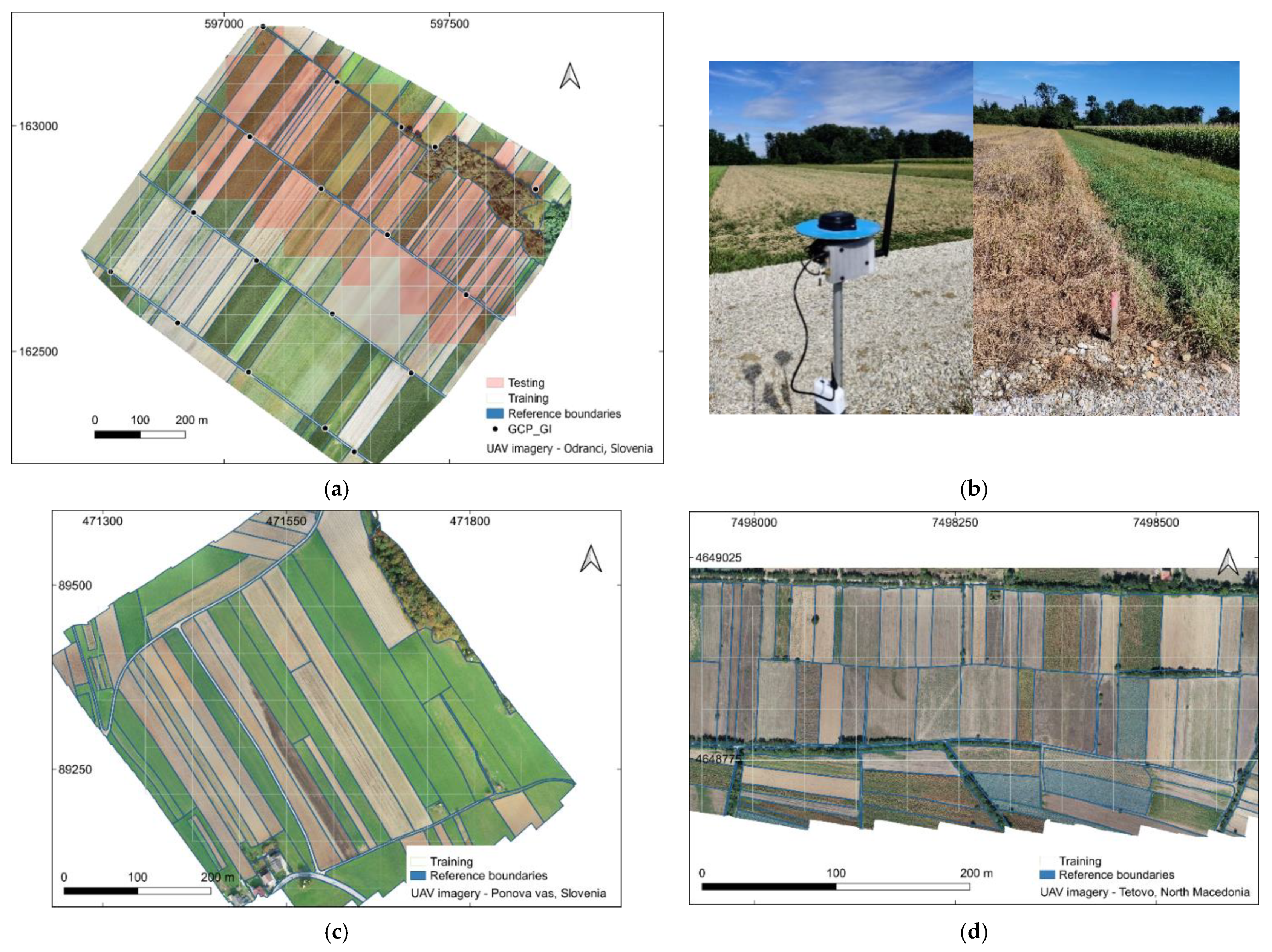
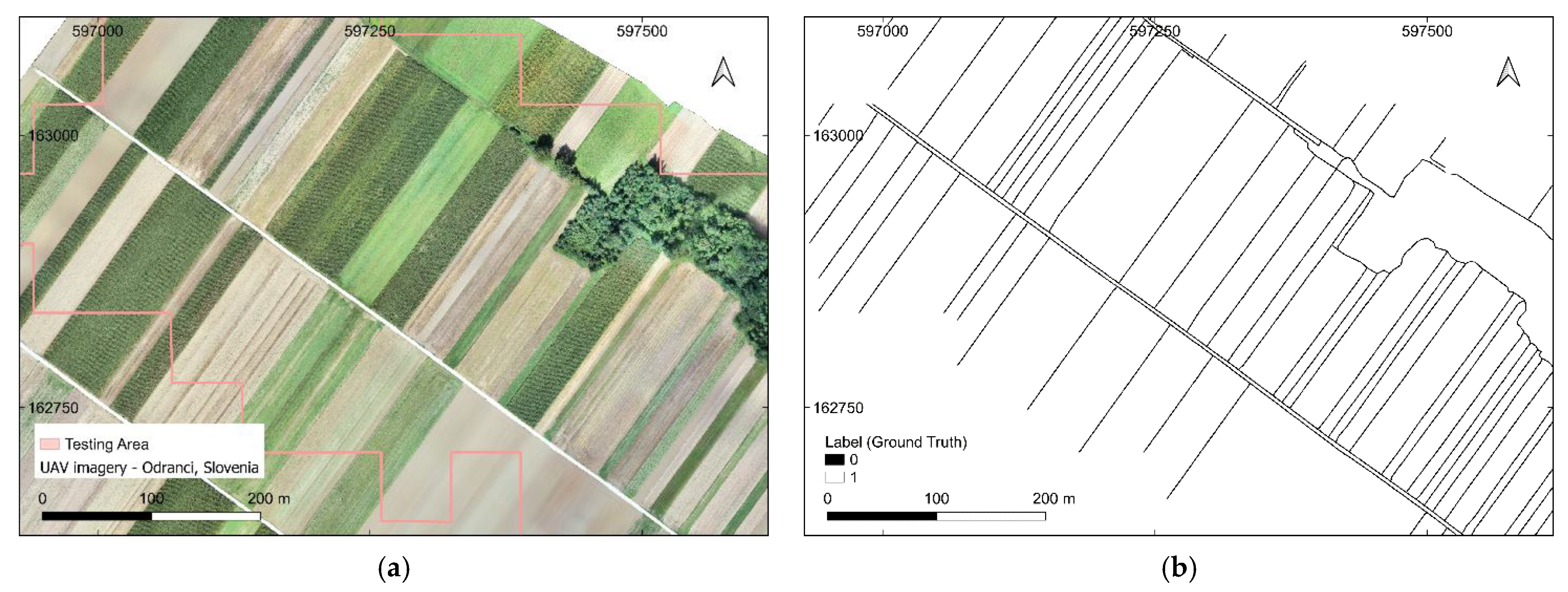
2.1. UAV Data

It is argued that the number of visible cadastral boundaries is higher in rural areas than in dense urban areas (an example of a visible cadastral boundary in Figure 1b). A rural area in Odranci, Slovenia, was selected for this study. UAV images were acquired at a flight altitude of 90 m, resulting in 997 images to cover the study area. The images were acquired in September 2020, at midday, under clear skies. The UAV images were indirectly georeferenced using a uniform distribution of 18 ground control points (GCPs). The GCPs were surveyed with real-time kinematic (RTK) using the global navigation satellite system (GNSS) receiver Leica GS18. In addition, the GCPs were also surveyed with RTK, using a multifrequency low-cost GNSS instrument (base and rover), namely ZED-F9P receiver with u-blox ANN-MB-00 antenna—as a cheaper alternative to geodetic GNSS receivers (Figure 1b). The differences were insignificant for 2D cadastral mapping (RMSE_x,y = 0.019 m). The obtained ground sampling distance (GSD) from the UAV orthoimage was 0.02 m. The study site had an area of 63.9 ha and was divided into areas for training and testing the CNNs (Figure 1a).

With the aim of increasing the number and diversity of training data, additional UAV images with a rural scene from Ponova vas (Slovenia) and Tetovo (North Macedonia) were used (Figure 1c,d). The UAV data in Ponova vas was acquired at an altitude of 80 m and had a GSD of 0.02 m. The UAV data in Tetovo have a GSD of 0.03 m and were acquired at an altitude of 110 m. Figure 1a,c,d shows the UAV orthoimages of the study areas.

The selected areas contain agricultural fields, roads, fences, hedges and tree groups, which are assumed to represent cadastral boundaries [8]. The cadastral reference boundaries were derived from the UAV orthoimages by manual land delineation on-screen in all three study areas. All UAV images were acquired using a rotary-wing UAV, namely the DJI Phantom 4 Pro.

Table 1. Specification of unmanned aerial vehicle (UAV) dataset for the selected study areas.

Location	UAV Model	Camera/Focal Length (mm)	Overlap Forward/Sideward	Flight Altitude	GSD (cm)	Coverage Area (ha)	Purpose
Odranci, Slovenia	DJI Phantom 4 Pro	1” CMOS/24 mm	80/70	90 m	2.35	63.9	Training and Testing
Ponova vas, Slovenia				80 m	2.01	25.0	Training
Tetovo, North Macedonia				110 m	2.85	24.3	Training

shows the specifications of the data acquisition.

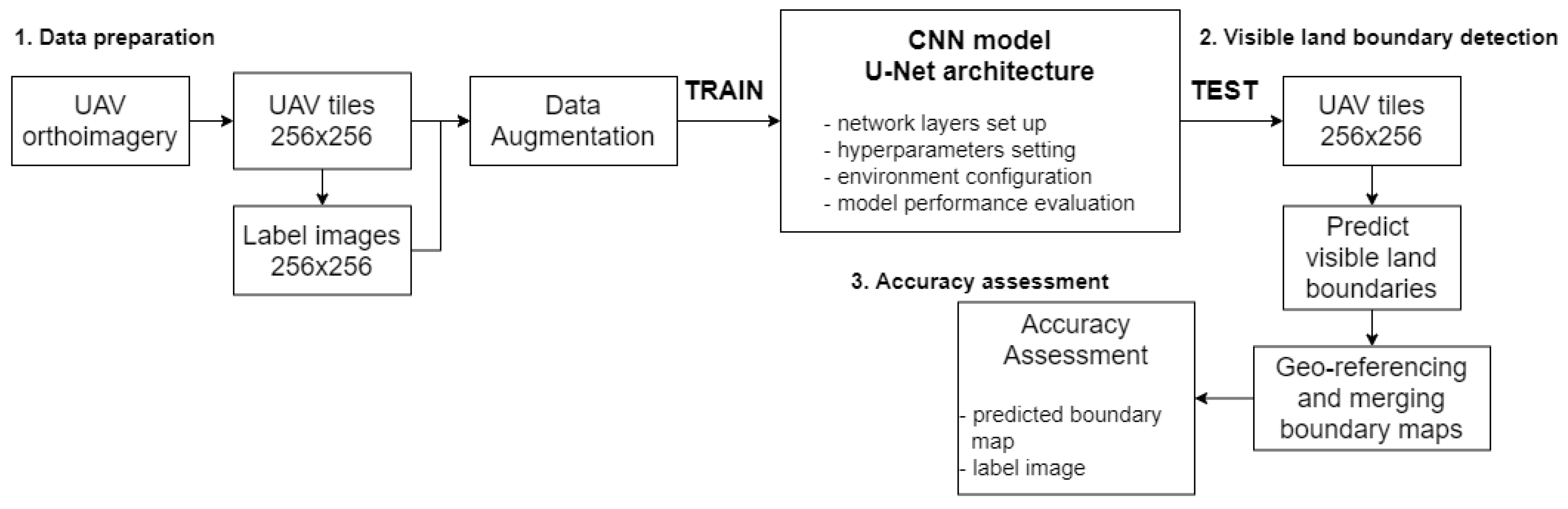
2.2. Detection of Visible Land Boundaries

In general, the workflow of this study consists of three main parts, namely data preparation, visible land boundary detection and accuracy assessment. The specific steps for both the U-Net and ENVI deep learning boundary mapping approaches are described in the following subsections.

2.2.1. U-Net

In deep learning, CNNs can be trained in two approaches, from scratch or via transfer learning [17,32]. In our case, the U-Net model was trained from scratch based on UAV images.

The UAV orthoimages of the selected study areas (Figure 1a–c) were randomly tiled in 256 pixels × 256 pixels. To increase the field of view for each tile, the original spatial resolution of the UAV orthoimages had to be converted to a larger GSD, from 2–3 to 25 cm. The results were 219 original tiles, namely 144 tiles for training and 75 tiles for testing (Figure 1a,c,d). In addition, corresponding label images (also called ground truth images) were created for each UAV image. The label images, with a size of 256 × 256 × 1, were created from the manually digitized reference boundaries, which were initially in the vector format. The reference boundaries were buffered to 50 cm and later rasterized using GRASS GIS tools [33]. Additionally, the UAV tiles were then rotated, flipped and scaled to improve generalization and increase the number of training samples. This technique is known in deep learning as data augmentation and is used to supplement original training data. Once the data preparation and augmentation were completed, the next step was to train the U-Net model.

The CNN based on U-Net is symmetric and contains encoding and decoding parts, which gives it the U-shaped form. U-Net is described in detail in [26]. The left part, the encoding path, is a typical convolutional network that contains repetitive usage of 3 × 3 convolutions, each followed by a rectified linear unit (ReLU) and a max-pooling operation, i.e., 2 × 2 convolutions. During the encoding path, the contextual information (depth) of the images was increased while the resolution of the images was reduced. The right part, the decoding path, merged the contextual and resolution information of the images through a sequence of 2 × 2 up-convolutions. The goal of the decoding path is to provide precise localization using the contextual information from the encoding path. During the decoding path, the resolution of the image was upconverted to its original size. The U-Net architecture implemented in this study is shown in Figure 2.

Overall, training a CNN model requires a powerful graphics processing unit (GPU), lots of memory and efficient computations. To overcome this requirement while providing a cost-effective and fast approach for visible boundary detection and hence cadastral mapping, the training of U-Net was performed by Google Collaboratory [34]. U-Net was implemented in the high-level neural network API Keras [35]. The process was written in Python in combination with the TensorFlow library [36]. The implementation of the model in Keras was done by modifying and referencing to [37], which is an implementation for grayscale biomedical images. In this study, the U-Net model was adapted to work with three-band images, namely RGB UAV images, as input and produce a single band boundary map as output with the same image size as the input. However, the predicted boundary maps were not georeferenced.

Considering that georeferencing is the key component in cadastral mapping, further improvements were made. In this study, we considered two additional steps, namely georeferencing the predicted boundaries and merging the georeferenced tiles to obtain the boundary map for the entire extent of the test area. The processing and analysis were done using open-source modules, including Rasterio [38], GDAL [39] and Numpy [40]. The workflow and boundary mapping approach used in this study are shown in Figure 3.

2.2.2. ENVI Deep Learning

ENVI deep learning [41] can be categorized as software-based deep learning technology that offers its own U-Net-like model. The model is called ENVINet5 and is described in detail in [42]. In this study, the ENVINet5 model was used to compare it with the U-Net model—both the results and the land boundary mapping approach.

The training approach is patch-based, i.e., the entire extent of the training UAV data can be used as input, and the model can learn based on the pixels specified in the patch. Considering this, a patch size of 256 pixels × 256 pixels was used for training and validating the ENVINet5 as a single-class model. Moreover, the training of the ENVINet5 model is based on a labelled raster that should be created within the software. Generally, there are two approaches: by on-screen manual digitizing or by directly uploading features in vector format. In our case, we uploaded the shapefile (.shp) of reference cadastral boundaries (buffered to 50 cm), defined as the region of interest (ROI), from which the label raster was created. We used the recently released version of ENVI deep learning, i.e., version 1.1.2, which has an option for data augmentation, unlike the previous version where data augmentation was not possible. Data augmentation is performed by rotating and scaling the original UAV training data.

The training of the ENVINet5 model was done using the toolbox deep learning guide map. Before starting the training, it was necessary to initialize a TensorFlow model, which defines the structure of the model, including the architecture (ENVINet5 for a single class), the patch size (256 × 256), and the number of the bands that are used for training (3 bands, RGB). After the model was initialized, the training data was uploaded. In the following, the values for the training parameters are required, such as the number of epochs, the number of patches per epoch, the number of patches per batch, class weight, etc. For the number of patches per epoch and per batch, it is suggested to leave them blank so that ENVI automatically determines the most appropriate values. For saving the model and the trained weights (output model), ENVI uses the HDF5 (.h5) format. The generated land boundary maps were georeferenced, and no post-processing step was required. The boundary mapping approach and workflow used in this study are shown in Figure 4.

However, there were some hardware and software requirements, such as NVIDIA GPU driver version 410.x or higher and NVIDIA graphics card with CUDA compute capability 3.5–7.5. Additionally, it is recommended to have at least 8 GB GPU memory to perform the training of the models with the GPU. If this requirement is not met, the training will be performed with the central processing unit (CPU), which is too slow for a large number of images.

2.3. Accuracy Assessment

The accuracy assessment in this study investigates two aspects—the evaluation of the two models U-Net and ENVINet5 and the evaluation of the detection quality of the visible land boundaries for the test UAV data (Figure 1a).

Both CNN models, U-Net and ENVINet5, were monitored with loss and accuracy during the training process. Loss is defined as the sum of errors for each sample in training between labels and predictions. To maximize the efficiency of the model, loss should be minimized. For this purpose, we used the cross-entropy loss expressed by the following formula:

$$cross-entropy loss=-\left(y_i\log ({\widehat{y}}_i\right)+\left(1-y_i\right)\log \left(1-{\widehat{y}}_i\right))$$

(1)

where:

$y_i$—actual label value,

${\widehat{y}}_i$—predicted value.

To assess the performance of the models, overall accuracy was used as the evaluation metric. The overall accuracy was calculated by summing the percentages of pixels correctly identified as land boundaries by the model compared to the labelled reference boundaries and dividing by all boundaries. Overall accuracy is expressed with the following equation:

$$overall accuracy=\frac{TP+TN}{TP+FP+FN+TN}$$

(2)

where true positive (TP), true negative (TN), false positive (FP) and false negative (FN) are shown in

Table 2. Confusion matrix.

Ground Truth
		Boundary	No Boundary
Prediction	Boundary	TP	FP
	No boundary	FN	TN

, which is the confusion matrix used to evaluate the detection quality of the visible land boundaries.

The detection quality of the visible land boundaries was evaluated by computing the F1 score derived from the confusion matrix. F1 score was calculated for test UAV data (not seen by the model during training) and represented the harmonic mean between recall and precision (Equations (3) and (4)). Larger values indicate higher accuracy.

$$recall=\frac{TP}{TP+FN}$$

(3)

$$precision=\frac{TP}{TP+FP}$$

(4)

The recall is the ratio of correctly predicted visible boundaries to all reference cadastral boundaries. The precision is the ratio of correctly predicted visible boundaries to all predicted positive visible boundaries. The F1 score combines precision and recall and is expressed with the following equation:

$$F1 score=2\ast \frac{recall\ast precision}{recall+precision}$$

(5)

3. Results

3.1. CNN Architecture

In our study, the labelled images and RGB UAV images were used to train the deep CNN models.

For the U-Net, the randomly cropped tiles (Figure 1a,c,d) were the candidate training datasets. The greater the variety of images used in the training data, the more robust the network and the better the detection of visible land boundaries. Data augmentation was applied to the provided images to increase the number of UAV images available for training the U-Net model. Of the data used for training, 30% was used for validation. Once the U-Net model was trained, we applied it to the test UAV images (Figure 1a).

The architecture was based on the original architecture of the U-Net, considering the number of layers (network depth) and the size of the convolutional filters. However, to avoid the resizing of the output image by the max-pooling operation, the padding was set to ‘same’. In addition, a dropout rate of 0.8 was used as an optional function. The dropout rate aims to avoid overfitting the model, which means that the training and validation accuracy curves are less likely to diverge, then the model is more robust. To avoid under-fitting, the layer depth was set to 1024. The larger the layer size, the higher the probability that the curve for validation will be close to the training accuracy. We used sigmoid instead of softmax as the final activation layer to retrieve the predictions, which is good for binary classification. The main point is that when using sigmoid, the probabilities were independent and did not necessarily sum to one. This is because the sigmoid considers each raw output value separately. During training, the optimization algorithm stochastic gradient descent (SGD) was used as the optimizer, and the momentum was set to 0.9. The learning rate in the optimization defines the speed of learning, which makes the network training converge. We used an adjusted learning rate of 0.001.

Table 3. Settings and adjusted parameters for our fine-tuned CNN based on the U-Net architecture.

	Settings	Parameters
Trainable layers	pooling layer	maxpooling 2D
	connected layer	layer depth = 1024 activation = ReLU
	dropout layer	dropout rate = 0.8
	logistic layer	activation layer = sigmoid
Learning optimizer	SGD optimizer	learning rate = 0.001 momentum = 0.9
Training	UAV images 256 × 256 × 3, data augmentation, validation split 0.3	number of epochs = 100 batch size = 32 steps per epoch = training samples/number of epochs

shows the adjusted settings and parameters.

The model was trained with a batch size of 32 for 100 epochs. An early stop function was also used to monitor validation loss. The number of steps per epoch was calculated by dividing the total number of training images by the batch size. Deep learning by the U-Net model was performed in Google Collaboratory, which provided a GPU with 25 GB of RAM. A total of 4768 samples, i.e., augmented images, were used for training and 2044 samples for validation. Training the model for 100 epochs took 4 h. The best model was saved at epoch 92 by achieving an overall accuracy of 0.978 and a loss of 0.058. The training performance of the U-Net is visualized in Figure 5.

In this study, we also used ENVI deep learning to compare the results obtained with the U-Net model. In this study, ENVI deep learning is considered a ‘black box’. The information we had is that ENVINet5 is based on U-Net architecture, and it uses the same layer size and the same number of convolution layers.

The ENVINet5 model was trained with a patch size equal to the total extent of the training UAV data. In addition, the training data shown in Figure 1a,c,d were also processed as UAV images for validation. The adapted training parameters of ENVINet5, namely patch size of 256 × 256, number of epochs 50 and class weights min. 1 and max. 2, data augmentation ‘yes’, resulted in a fine-tuned model for visible boundary detection. The values of the other parameters were automatically filled by ENVI deep learning as they are suggested to be left blank. The model with the best performance was saved at epoch 24, where the validation loss reached its lowest value. The overall accuracy of the model was 0.946 and with a loss of 0.234. The training performance of the CNN model ENVINet5 is shown in Figure 6.

All experiments with ENVI deep learning were performed on an Intel^® Core ™ i7-4771 CPU 3.5 GHz machine with an NVIDIA GeForce GTX 650 GPU with 2 GB of RAM. The training time for 50 epochs was 6 h.

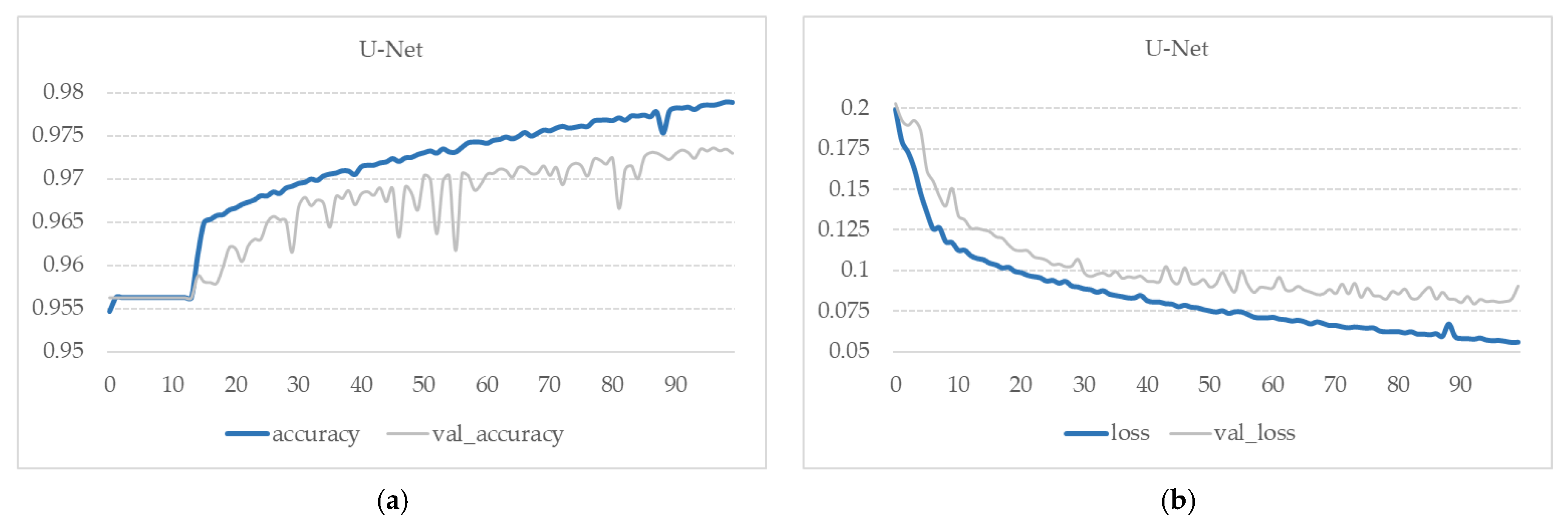
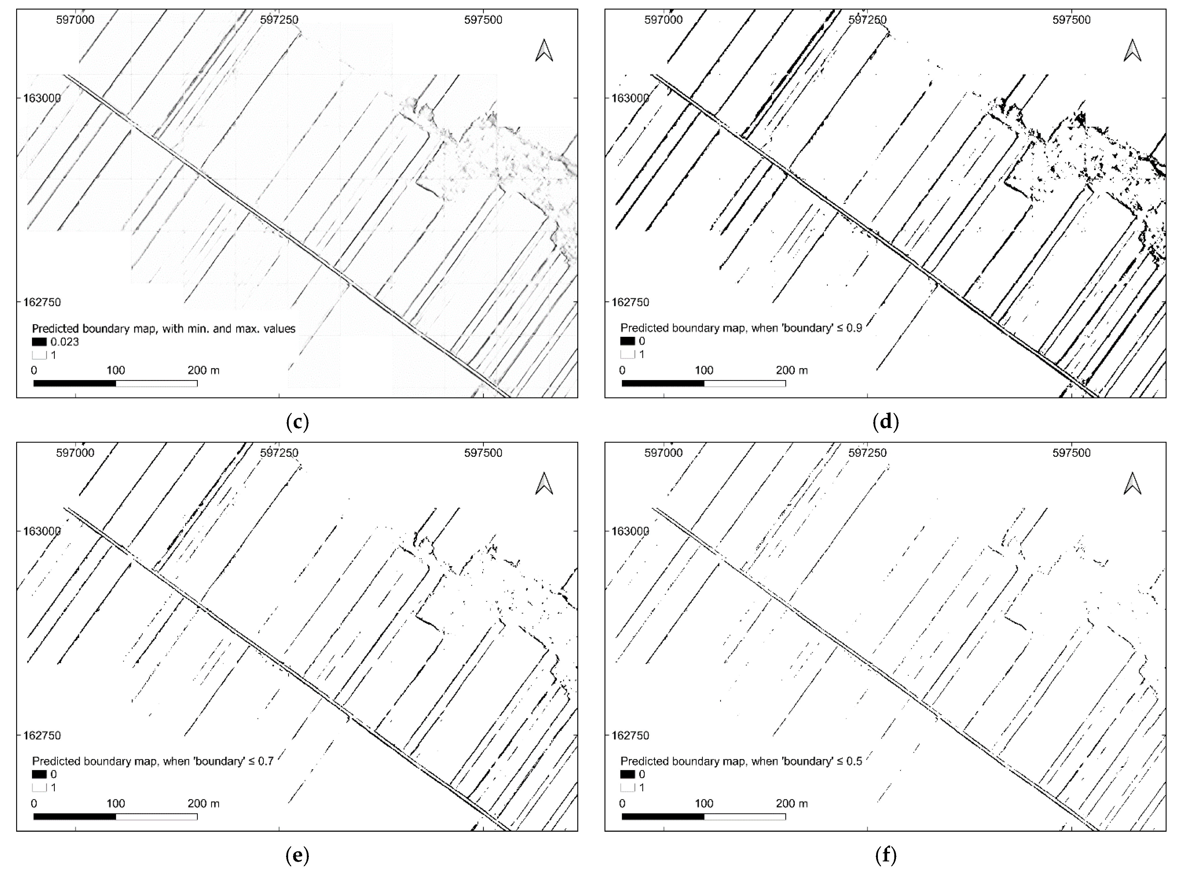
3.2. Detection of Visible Land Boundaries by U-Net

After training the CNN model, we evaluated its performance by applying it to the test area (Figure 1a). We applied the trained U-Net model to the test UAV tiles of size 256 × 256 to predict the visible land boundaries. Some results of the predicted boundary maps based on UAV tiles are shown in Figure 7.

The next step was to georeference the predicted visible land boundaries and merge them into a single land boundary map (Figure 8c). Considering that the predicted values were in the range of 0–1, in order to assess the accuracy and thus match the ground truth class values, it was necessary to reclassify the predicted values to 0 and 1, namely to ‘boundary’ and ‘no boundary’. In this study, few boundary map reclassifications were performed, e.g., ‘boundary’ ≤ 0.9; ‘boundary’ ≤ 0.7; ‘boundary’ ≤ 0.5. The predicted boundary maps for the test area showed a good match with the labelling image (ground truth). The results of the georeferenced and merged predictions along with the reclassified boundary maps are shown in Figure 8c–f.

For a quantitative description of the predicted boundary maps, overall accuracy, F1 score, recall and precision are summarized in

Table 4. Accuracy assessment of visible land boundary detection with U-Net.

Predicted Boundary Map	Overall Accuracy (%)	Recall	Precision	F1 Score
Boundary ≤ 0.9	94.5	0.654	0.413	0.506
Boundary ≤ 0.7	96.2	0.480	0.565	0.519
Boundary ≤ 0.5	96.5	0.348	0.675	0.459

. Overall accuracy represents a general metric by counting true positives/negatives and false positives/negatives, i.e., it considers both ‘boundary’ and ‘no boundary’ classes. All predicted boundary maps resulted in an overall accuracy of over 94%. To get a better insight into the detection quality, F1 score, recall and precision were calculated for the class’ boundary’ or ‘0’ as a positive class. The results showed that more relevant visible land boundaries were detected when the predicted boundary map was reclassified with the threshold ‘boundary’ ≤ 0.9, resulting in an F1 score of 0.51. More balanced scores were retrieved for the boundary map with ‘boundary’ ≤ 0.7, resulting in an F1 score of 0.52. Higher precision was obtained for the boundary map with the reclassification threshold ‘boundary’ ≤ 0.5, resulting in an F1 score of 0.46.

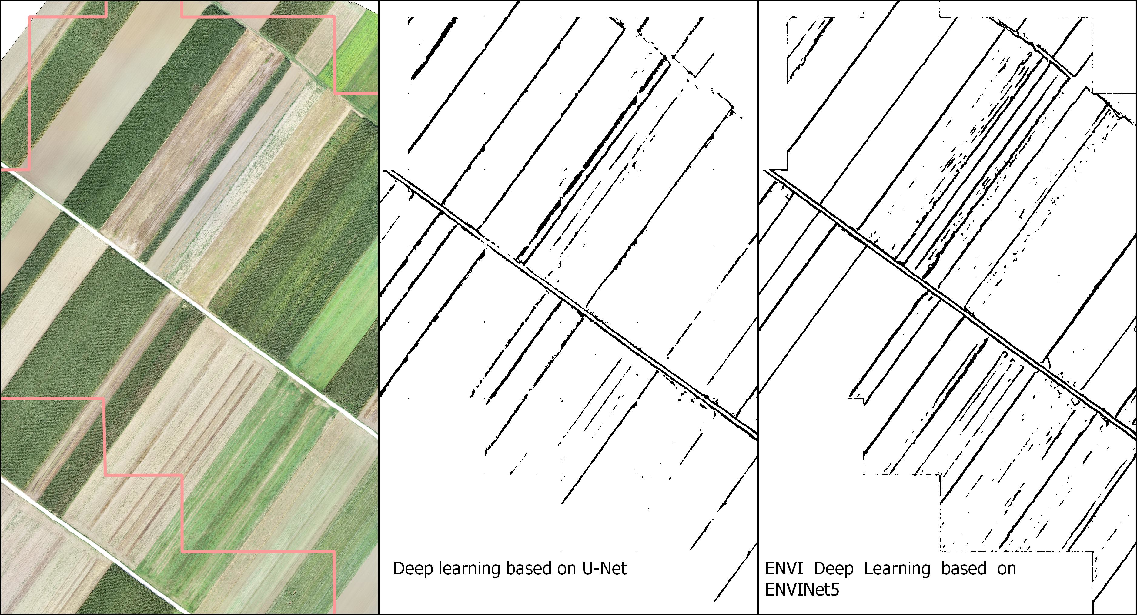
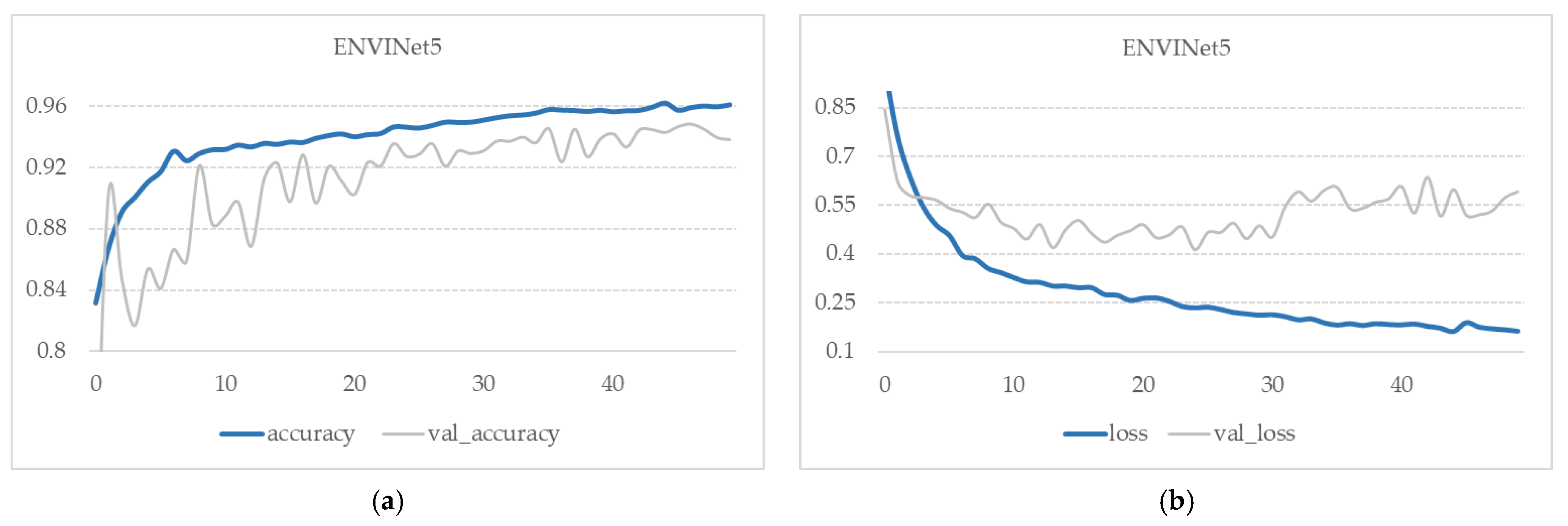
3.3. Comparison with ENVI Deep Learning—ENVINet5

The predicted land boundary map for the test area (Figure 8a) retrieved using ENVINet5 model was already georeferenced, so no further post-processing step was required. In addition, the retrieved boundary map contained predicted values of 0 and 1, and no additional reclassification step was performed to compare the results to the ground truth map and to assess accuracy. The predicted boundary is visualized in Figure 9b.

Considering that all predictions retrieved with ENVINet5 were assigned the prediction value 0 for the class’ boundary’, we selected the boundary map for the comparison of results with U-Net, where all predictions ≤0.9, were reclassified as 0—‘boundary’. With this, we wanted to compare predictions from U-Net that were as close as possible to the predictions of ENVINet5. The overall accuracy was 94.5% for U-Net and 96.2% for ENVINet5. However, in terms of detection quality for the ‘boundary’ class, ENVINet5 showed higher recall and lower precision than U-Net. In short, F1 score showed a slightly higher value for U-Net, i.e., 0.51 compared to ENVNet5, where the value was 0.49. The confusion matrices are shown in

Table 5. Confusion matrices based on the number of pixels.

Ground Truth
		Boundary	No Boundary
U-Net	Boundary	137,056	195,156
	No boundary	72,524	8,966,912
ENVINet5	Boundary	175,559	325,076
	No boundary	34,021	8,836,992

and the quantitative results in

Table 6. Accuracy assessment and comparison with ENVINet5.

Predicted Boundary Map	Overall Accuracy (%)	Recall	Precision	F1 Score
U-Net	94.5	0.654	0.413	0.506
ENVINet5	96.2	0.838	0.351	0.494

.

4. Discussion

Deep learning is a relatively new research area and offers great potential for feature detection from remote sensing imagery [21,24]. The application of CNNs for detecting visible land boundaries is becoming increasingly important, especially for UAV-based cadastral mapping. In this work, we presented a deep learning application using Python with Keras to implement U-Net, and software-based ENVI deep learning for visible land boundary detection from UAV imagery. The research obtained encouraging and reasonable results that can help to automate the process of cadastral mapping.

4.1. CNN Architecture and Implementation

In both network models, the loss was constantly decreasing from the first epoch until the end. This indicated that the model was still learning on training samples. However, the training of the models was monitored with the validation loss to avoid overfitting. The training performance of the network models was shown in Figure 5 and Figure 6. The validation loss for U-Net was decreasing until epoch 92 and for ENVINet5 until epoch 24. This was a good sign that the model did not lose the ability to generalize predictions for test datasets that were not seen by the model during training. The evaluation metric showed relatively high accuracies, 0.978 for U-Net and 0.946 for ENVINet5. The high accuracy of the network models, including the first epochs, is mainly due to the unbalanced pixels of the classes. The land boundaries occupy a minimal number of pixels compared to the background pixels.

In this study, we used a deep learning-based visible land boundary detector. Here, providing balanced pixels for ‘boundary’ and ‘no boundary’ is a bit challenging, especially for UAV imagery. UAV imagery usually has a small GSD (2–5 cm) and a limited coverage area beside the efficient and flexible data acquisition system [14]. Moreover, the number of background pixels in cadastral maps is always much higher than the number of pixels representing the course of the cadastral boundaries themselves (line-based). The imbalance of pixels per class is even more evident in randomly cropped tiles from UAV imagery. Resampling the original GSD to a larger GSD contributed somewhat to an increase in the field of view and balance between classes. However, the size of the GSD and the number of training tiles is limited by the coverage area. To increase the amount of training data, we applied data augmentation. Data augmentation has proven to be an efficient technique to supplement original UAV training data, especially when training the U-Net model from scratch. However, it remains a challenge to confirm what should be a sufficient variety of UAV training data to learn a robust network model for visible cadastral boundary detection.

The problem of unbalanced classes could be solved by rebalancing the class weights, using additional evaluation metrics besides overall accuracy, or performing deep learning with multiple classes for land cover (polygon-based). In addition, other remote sensing imagery can be used for the training data, e.g., aerial or satellite imagery; imageries can be cropped in a way to cover more balanced pixels for ‘boundary’ and ‘no boundary’ and may not be limited with the coverage area. This can be applied if the deep learning model is to be trained using only cadastral data that requires manual data preparation, such as the creation of image tiles and corresponding ground truths. Instead, the CNN model could be trained via transfer learning, similar to [17]. To avoid ambiguity, the detection quality for UAV test data in this study was evaluated using recall, precision and F1 score for the class ‘boundary’. Thus, we had two indicators, overall accuracy, which includes both ‘boundary’ and ‘no boundary’ classes and one that is specific only to the ‘boundary’ class. Although both models performed well, there were significant differences in implementation and training, as one approach is customized, e.g., U-Net, and is offered as an API, while the other, e.g., ENVINet5, is software-based, where we have fewer parameters available but can still achieve good results.

Training a deep learning model requires more memory, a stronger GPU and efficient computation. Training of the U-Net model was performed in Google Collaboratory, which is open-source and can be considered as an alternative for the hardware costs to get more memory and a more powerful GPU. On the other hand, ENVI deep learning had some hardware and software requirements to perform the training of the network model. Google Collaboratory allowed faster training compared to our machine. For 100 epochs, the training time was 4 h with Google Collaboratory and three times the training time with ENVI deep learning since it was run on a local machine with less computational power. It should be emphasized that ENVI deep learning provided more stable training in terms of a training session interruption, which occasionally happened with Google Collaboratory.

4.2. Detection of Visible Land Boundaries

The network models, both U-Net and ENVINet5, generally performed well in detecting visible land boundaries, with some exceptions in the forest area. The results of the quality of visible land boundary detection are shown in Figure 8 and Figure 9 and quantitatively in Table 4 and Table 6. The results show that most visible land boundaries were correctly detected, which demonstrates the ability of the UAV imagery and network models to detect these types of land boundaries, especially in rural areas.

U-Net generated boundary maps with low recall and high precision when the threshold for ‘boundary’ was set ≤0.5. This resulted in a recall of 0.35 and a precision of 0.68. More balanced results and a higher F1 score were obtained when the threshold for ‘boundary’ was set ≤0.7, namely a recall of 0.48, precision of 0.57 and F1 score of 0.52. The boundary map with high recall and low precision was generated when the threshold was set almost to the maximum, namely ‘boundary’ ≤ 0.9. This boundary map was used for comparison with the new map obtained with ENVINet5, since nearly all predictions were reclassified to the ‘boundary’ class, which is in accordance with the output of ENVINet5.

The results show an overall accuracy of 94% and 96% for U-Net and ENVINet5, respectively. However, for the ‘boundary’ class, U-Net gave 0.51 F1 score and ENVINet5 0.49. This is mainly because U-Net provided more balanced scores, namely 0.65 in recall and 0.41 in precision. On the other hand, ENVINet5 provided higher recall (0.84) and lower precision (0.35), which means that the ‘boundary’ class is well detected, but the model also includes points of the background class in it.

U-Net provided boundary maps that were in the range of 0–1. This is due to the chosen sigmoid function as the activation function of the output layer, where the output values obtained are estimates of the probability that the input belongs to class ‘boundary’. Then, we set a threshold to decide whether the input belongs to class ‘boundary’ or class ‘no boundary’. The results maintain a balance; the lower the threshold, the lower the recall and the higher the precision. The significant point of the threshold is that the same can be used as a filtering method for boundary maps, depending on the need and purpose of the application. For example, a low threshold provided high precision, while a high threshold provided high recall. The recall is also referred to as completeness, while the precision is referred to as correctness [15]. Imbalanced classes are common in cadastral maps, and when it comes to specific use cases, more importance should be given to the metrics recall and precision, and how a balance between them can be achieved—which in our case was supported by filtering the predicted boundary maps (Figure 8e). Unlike U-Net, ENVINet5 provided all predictions with values 0 and 1, and no further thresholding or filtering could be applied.

In cadastral mapping, it is desirable that the relevant or candidate boundaries are correctly extracted since the correct determination of the location of the cadastral boundaries is the core of the cadastre itself (correctness). On the other hand, increasing the number of possible boundaries increases the cadastral coverage (completeness). Considering this, a model that provides a balance between recall and precision is preferable. In short, a model that provides a high F1 score.

The comparison of the results obtained with U-Net with other studies, in particular [15,17,25], which deal with the automation of cadastral mapping using different CNN architectures, is not possible at this stage. This is mainly because the training approach of the network models along with the input training data differs from study to study. Thus, a reliable and qualitative comparison is not possible.

4.3. Boundary Mapping Approach

This section refers to the visible land boundary detection workflows applied in custom-based U-Net and software-based ENVI deep learning. In general, boundary mapping approaches are quite different, starting from data preparation to the final predicted boundary map. However, these differences provide advantages and disadvantages for each boundary mapping approach used in this study.

In general, programming-based deep learning is open-source and offers a more flexible but complex approach compared to software-based deep learning. Software-based deep learning, e.g., ENVI deep learning, is simpler but at the same time more rigid. For example, U-Net can be trained in a machine and in online platforms such as Google Collaboratory, where the hyperparameters can be configured individually. In contrast, ENVI deep learning has no implementation choices, but it also requires no additional configuration. The latter can be considered a very important aspect as not all land administrators are experts in programming, and this can be an option for them to perform deep learning. The main challenge with CNNs is the preparation of a large amount of training data [26], especially when the goal is to train the network only cadastral data [17]. In order to increase the amount of training data for the U-Net, it was necessary to decompose the UAV orthoimages in tiles before data augmentation. Moreover, for each UAV tile, a corresponding label image (ground truth) was manually created using additional software for rasterisation. In contrast, training in ENVI deep learning was patch-based, and the entire extent or a larger UAV tile can be used as input for training. In addition, the labelling images were created quite quickly within the software—directly by uploading reference boundaries as ROIs. The boundary maps retrieved using U-Net were the same size as the input but were not georeferenced. Considering that georeferencing is the key element in cadastral mapping, it was necessary to georeference and merge predicted boundary maps from the test UAV tiles. In ENVI deep learning, the prediction boundary map was already georeferenced, and the predictions had values of 0 and 1. Therefore, further filtering of the predicted boundary maps was not possible. The advantages and disadvantages of the U-Net and ENVI deep learning mapping approaches used in this study are summarized in

Table 7. Summarized advantages (pros) and disadvantages (cons) for boundary mapping approaches used in this study.

U-Net		ENVI Deep Learning
pros	cons	pros	cons
open-source	programming	no programming	commercial
impl. online or on machine	additional georeferencing step	georeferencing	impl. on machine only
hyper-parameter configuration	label image manually	label image by software	hyper-parameter configuration
prediction values in range; filtering of boundary maps			fixed predictions

.

4.4. Application of Detected Visible Boundaries

Cadastral boundaries are often demarcated by objects visible in remote sensing imagery [2,8]. Automatic detection of cadastral boundaries based on remote sensing imagery, especially UAV imagery, has rarely been investigated. Automatic extraction of visible land boundaries, i.e., property boundaries, offers the potential to improve current approaches to cadastral mapping. The boundary mapping approaches investigated are based on deep learning and offer improvements in terms of time and cost.

Both boundary mapping approaches, i.e., U-Net and ENVI deep learning, can help to facilitate and accelerate cadastral mapping, especially in areas where large parts of the cadastral boundaries are continuous and visible. In terms of delineation effort per parcel, automatic delineation approaches (including post-alignments) require up to 40% less time in rural areas compared to manual delineation, based on [17]. However, in areas where cadastral boundaries are not visible in the image, manual delineation remains superior. Overall, it can be said that manual methods provide slower but more accurate delineations, while automatic methods are faster but less accurate (once the model is trained).

In countries with low cadastral coverage, deep learning-based mapping approaches can be used to produce cadastral maps. In countries with full cadastral coverage, the detected visible boundaries can be used to automate the process of revising the up-to-dateness of existing cadastral maps. In this way, areas requiring updating and improving cadastral boundary maps can be automatically identified. Notwithstanding the advances in cadastral mapping, the automation of cadastral boundary detection is still ongoing [15,17,18]. This is due to the nature of cadastral boundaries, which may have a simple geometry but are very complex to interpret. Consequently, automatically detected visible land boundaries should be considered as preliminary cadastral boundaries. Verification of automatically detected land boundaries should be aligned with the existing technical, legal and institutional framework of land administration. Moreover, not every cadastral boundary is demarcated with visible objects. In this study, boundary mapping approaches were tested in rural areas. It is argued that the number of visible cadastral boundaries is higher compared to urban areas [2].

Automating the detection of invisible cadastral boundaries remains a challenge in land administration, which has already been highlighted in [17]. Future work could investigate and analyze the applicability of deep learning for invisible cadastral boundaries that are marked prior to the UAV survey. It should be further investigated which type and size of land boundary markers are more appropriate for demarcating the invisible boundaries.

5. Conclusions

Deep learning is becoming increasingly important in cadastral applications as a state-of-the-art method for automatic boundary detection. The aim of this study was to investigate the potential of CNN architecture, namely U-Net, based on UAV imagery training samples—as a deep learning-based detector for visible land boundaries. The results and land boundary mapping approach using U-Net were compared with software-based ENVI deep learning. The overall accuracy for both CNN models was higher than 95%. This indicates that deep learning-based land boundary detection usually faces an unbalanced distribution of pixels per class, namely for ‘boundary’ and ‘no boundary’.

Regarding the quality of recognition for the class ‘boundary’ in the case of U-Net, we obtained low recall and high precision when the threshold ‘boundary’ ≤ 0.5 was set. This resulted in a recall of 0.35 and a precision of 0.68. Prediction reclassification can be considered as a tool to filter the predicted boundary maps. For example, to compare the results with ENVINet5, the threshold had to be set almost to its maximum. Here, U-Net provided a recall of 0.65 and a precision of 0.41. For ENVI deep learning, we obtained a recall of 0.84 and a precision of 0.35. Based on the F1 score (U-Net 0.51 and ENVI deep learning 0.49), U-Net provided slightly better and more balanced results. The predicted land boundary maps obtained with U-Net were georeferenced and merged in an additional post-processing step. This was not an issue with ENVI deep learning—the output boundary maps were already georeferenced. Overall, U-Net is a programming-based solution and provides a more flexible boundary mapping approach in terms of hyperparameters and CNN model setting. On the other hand, it can be somewhat complex and demanding for the practice as not all land administrators are skilled in programming. In contrast, ENVI deep learning does not require any programming and deep learning is guided by the software process.

While programming-based deep learning is challenging due to the complexity of the processes and their control, commercial software-based deep learning brings some abstraction but at the same time has limitations in terms of influencing the processes flow. Both land boundary mapping approaches investigated in our study can be used to accelerate and facilitate cadastral mapping in rural areas. However, the automatically detected visible land boundaries should be considered as preliminary boundaries for cadastral map production and updating. The results should be further aligned with technical, legal and institutional framework of land administration.

References

1. Enemark, S.; Bell, K.C.; Lemmen, C.; McLaren, R. Fit-For-Purpose Land Administration; International Federation of Surveyors (FIG): Copenhagen, Denmark, 2014; ISBN 978-87-92853-11-0. [Google Scholar]
2. Luo, X.; Bennett, R.; Koeva, M.; Lemmen, C.; Quadros, N. Quantifying the Overlap between Cadastral and Visual Boundaries: A Case Study from Vanuatu. Urban Sci. 2017, 1, 32. [Google Scholar] [CrossRef] [Green Version]
3. Zevenbergen, J. A systems approach to land registration and cadastre. Nord. J. Surv. Real Estate Res. 2004, 1, 11–24. [Google Scholar]
4. Simbizi, M.C.D.; Bennett, R.M.; Zevenbergen, J. Land tenure security: Revisiting and refining the concept for Sub-Saharan Africa’s rural poor. Land Use Policy 2014, 36, 231–238. [Google Scholar] [CrossRef]
5. Williamson, I.P. Land Administration for Sustainable Development, 1st ed.; ESRI Press Academic: Redlands, CA, USA, 2010; ISBN 9781589480414. [Google Scholar]
6. Binns, B.O.; Dale, P.F. Cadastral Surveys and Records of Rights in Land; Food and Agriculture Organization of the United Nations: Rome, Italy, 1995; ISBN 9251036276. [Google Scholar]
7. Grant, D.; Enemark, S.; Zevenbergen, J.; Mitchell, D.; McCamley, G. The Cadastral triangular model. Land Use Policy 2020, 97, 104758. [Google Scholar] [CrossRef]
8. Crommelinck, S.; Bennett, R.; Gerke, M.; Nex, F.; Yang, M.; Vosselman, G. Review of Automatic Feature Extraction from High-Resolution Optical Sensor Data for UAV-Based Cadastral Mapping. Remote Sens. 2016, 8, 689. [Google Scholar] [CrossRef] [Green Version]
9. Zevenbergen, J.; Bennett, R. The visible boundary: More than just a line between coordinates. In Proceedings of the GeoTech Rwanda, Kigali, Rwanda, 18–20 November 2015; pp. 1–4. [Google Scholar]
10. Manyoky, M.; Theiler, P.; Steudler, D.; Eisenbeiss, H. Unmanned Aerial Vehicle in Cadastral Applications. Int. Arch. Photogramm. Remote Sens. Spat. Inf. Sci. 2011, 57–62. [Google Scholar] [CrossRef] [Green Version]
11. Puniach, E.; Bieda, A.; Ćwiąkała, P.; Kwartnik-Pruc, A.; Parzych, P. Use of Unmanned Aerial Vehicles (UAVs) for Updating Farmland Cadastral Data in Areas Subject to Landslides. ISPRS Int. J. Geo-Inf. 2018, 7, 331. [Google Scholar] [CrossRef] [Green Version]
12. Koeva, M.; Muneza, M.; Gevaert, C.; Gerke, M.; Nex, F. Using UAVs for map creation and updating. A case study in Rwanda. Surv. Rev. 2018, 50, 312–325. [Google Scholar] [CrossRef] [Green Version]
13. Stöcker, C.; Nex, F.; Koeva, M.; Gerke, M. High-Quality UAV-Based Orthophotos for Cadastral Mapping: Guidance for Optimal Flight Configurations. Remote Sens. 2020, 12, 3625. [Google Scholar] [CrossRef]
14. Colomina, I.; Molina, P. Unmanned aerial systems for photogrammetry and remote sensing: A review. ISPRS J. Photogramm. Remote Sens. 2014, 92, 79–97. [Google Scholar] [CrossRef] [Green Version]
15. Xia, X.; Persello, C.; Koeva, M. Deep Fully Convolutional Networks for Cadastral Boundary Detection from UAV Images. Remote Sens. 2019, 11, 1725. [Google Scholar] [CrossRef] [Green Version]
16. Ramadhani, S.A.; Bennett, R.M.; Nex, F.C. Exploring UAV in Indonesian cadastral boundary data acquisition. Earth Sci. Inf. 2018, 11, 129–146. [Google Scholar] [CrossRef]
17. Crommelinck, S.; Koeva, M.; Yang, M.Y.; Vosselman, G. Application of Deep Learning for Delineation of Visible Cadastral Boundaries from Remote Sensing Imagery. Remote Sens. 2019, 11, 2505. [Google Scholar] [CrossRef] [Green Version]
18. Fetai, B.; Oštir, K.; Kosmatin Fras, M.; Lisec, A. Extraction of Visible Boundaries for Cadastral Mapping Based on UAV Imagery. Remote Sens. 2019, 11, 1510. [Google Scholar] [CrossRef] [Green Version]
19. Crommelinck, S.; Bennett, R.; Gerke, M.; Yang, M.; Vosselman, G. Contour Detection for UAV-Based Cadastral Mapping. Remote Sens. 2017, 9, 171. [Google Scholar] [CrossRef] [Green Version]
20. Arbeláez, P.; Maire, M.; Fowlkes, C.; Malik, J. Contour detection and hierarchical image segmentation. IEEE Trans. Pattern Anal. Mach. Intell. 2011, 33, 898–916. [Google Scholar] [CrossRef] [Green Version]
21. Ma, L.; Liu, Y.; Zhang, X.; Ye, Y.; Yin, G.; Johnson, B.A. Deep learning in remote sensing applications: A meta-analysis and review. ISPRS J. Photogramm. Remote Sens. 2019, 152, 166–177. [Google Scholar] [CrossRef]
22. Zhu, X.X.; Tuia, D.; Mou, L.; Xia, G.-S.; Zhang, L.; Xu, F.; Fraundorfer, F. Deep Learning in Remote Sensing: A Comprehensive Review and List of Resources. IEEE Geosci. Remote Sens. Mag. 2017, 5, 8–36. [Google Scholar] [CrossRef] [Green Version]
23. Persello, C.; Stein, A. Deep Fully Convolutional Networks for the Detection of Informal Settlements in VHR Images. IEEE Geosci. Remote Sens. Lett. 2017, 14, 2325–2329. [Google Scholar] [CrossRef]
24. Pan, Z.; Xu, J.; Guo, Y.; Hu, Y.; Wang, G. Deep Learning Segmentation and Classification for Urban Village Using a Worldview Satellite Image Based on U-Net. Remote Sens. 2020, 12, 1574. [Google Scholar] [CrossRef]
25. Park, S.; Song, A. Discrepancy Analysis for Detecting Candidate Parcels Requiring Update of Land Category in Cadastral Map Using Hyperspectral UAV Images: A Case Study in Jeonju, South Korea. Remote Sens. 2020, 12, 354. [Google Scholar] [CrossRef] [Green Version]
26. Ronneberger, O.; Fischer, P.; Brox, T. U-Net: Convolutional Networks for Biomedical Image Segmentation. 2015. Available online: http://arxiv.org/pdf/1505.04597v1 (accessed on 24 February 2021).
27. Diakogiannis, F.I.; Waldner, F.; Caccetta, P.; Wu, C. ResUNet-a: A deep learning framework for semantic segmentation of remotely sensed data. ISPRS J. Photogramm. Remote Sens. 2020, 162, 94–114. [Google Scholar] [CrossRef] [Green Version]
28. Flood, N.; Watson, F.; Collett, L. Using a U-net convolutional neural network to map woody vegetation extent from high resolution satellite imagery across Queensland, Australia. Int. J. Appl. Earth Obs. Geoinf. 2019, 82, 101897. [Google Scholar] [CrossRef]
29. Zhao, X.; Yuan, Y.; Song, M.; Ding, Y.; Lin, F.; Liang, D.; Zhang, D. Use of Unmanned Aerial Vehicle Imagery and Deep Learning UNet to Extract Rice Lodging. Sensors 2019, 19, 3859. [Google Scholar] [CrossRef] [Green Version]
30. Alshaikhli, T.; Liu, W.; Maruyama, Y. Automated Method of Road Extraction from Aerial Images Using a Deep Convolutional Neural Network. Appl. Sci. 2019, 9, 4825. [Google Scholar] [CrossRef] [Green Version]
31. Wierzbicki, D.; Matuk, O.; Bielecka, E. Polish Cadastre Modernization with Remotely Extracted Buildings from High-Resolution Aerial Orthoimagery and Airborne LiDAR. Remote Sens. 2021, 13, 611. [Google Scholar] [CrossRef]
32. Wani, M.A.; Bhat, F.A.; Afzal, S.; Khan, A.I. Advances in Deep Learning; Springer: Singapore, 2020; ISBN 978-981-13-6793-9. [Google Scholar]
33. GRASS Development Team. GRASS GIS Bringing Advanced Geospatial Technologies to the World; GRASS: Beaverton, OR, USA, 2020. [Google Scholar]
34. Google Colaboratory. Available online: https://colab.research.google.com (accessed on 29 April 2021).
35. Chollet, F.; et al. Keras. 2015. Available online: https://keras.io (accessed on 29 April 2021).
36. Martin, A.; Ashish, A.; Paul, B.; Eugene, B.; Zhifeng, C.; Craig, C.; Greg, S.C.; Andy, D.; Jeffrey, D.; Matthieu, D.; et al. TensorFlow: Large-Scale Machine Learning on Heterogeneous Systems. 2015. Available online: https://www.tensorflow.org/ (accessed on 29 April 2021).
37. Zhixuhao. Unet for Image Segmentation. Available online: https://github.com/zhixuhao/unet (accessed on 24 February 2021).
38. Gillies, S. Rasterio: Geospatial Raster I/O for Python Programmers. 2013. Available online: https://github.com/mapbox/rasterio (accessed on 30 April 2021).
39. GDAL/OGR Contributors. GDAL/OGR Geospatial Data Abstraction Software Library. 2021. Available online: https://gdal.org (accessed on 30 April 2021).
40. Harris, C.R.; Millman, K.J.; van der Walt, S.J.; Gommers, R.; Virtanen, P.; Cournapeau, D.; Wieser, E.; Taylor, J.; Berg, S.; Smith, N.J.; et al. Array programming with NumPy. Nature 2020, 585, 357–362. [Google Scholar] [CrossRef]
41. Exelis Visual Information Solutions. In ENVI Deep Learning; L3Harris Geospatial: Boulder, CO, USA, 1977.
42. Exelis Visual Information Solutions. ENVI Deep Learning—Training Background. Available online: https://www.l3harrisgeospatial.com/docs/BackgroundTrainDeepLearningModels.html (accessed on 9 March 2021).
Figure 1. (a) UAV imagery of 0.25 ground sample distance (GSD) for Odranci–Slovenia, divided into areas for training and testing; (b) low-cost instrument ZED-F9P and example of visible cadastral boundaries. (c) UAV imagery of 0.25 (GSD) for Ponova vas—Slovenia, used for training; (d) UAV imagery of 0.25 (GSD) for Tetovo—North Macedonia, used for training.
Remotesensing 13 02077 g001
Figure 2. The implemented U-Net architecture (adapted from [26]).
Remotesensing 13 02077 g002
Figure 3. Workflow for the detection of visible land boundaries based on the U-Net model.
Remotesensing 13 02077 g003
Figure 4. Workflow for the detection of visible land boundaries based on the ENVINet5 model.
Remotesensing 13 02077 g004
Figure 5. Model performance: (a) accuracy and (b) loss for our fine-tuned U-Net.
Remotesensing 13 02077 g005
Figure 6. Model performance: (a) accuracy and (b) loss for our fine-tuned ENVINet5.
Remotesensing 13 02077 g006
Figure 7. (a) Examples of UAV testing tiles; (b) label images; (c) predicted boundary maps with values 0–1.
Remotesensing 13 02077 g007
Figure 8. (a) Test UAV area; (b) label image; (c) predicted boundary map (0–1); reclassified boundary maps when (d) ‘boundary’≤ 0.9; (e) ‘boundary’≤ 0.7; (f) ‘boundary’≤ 0.5.
Remotesensing 13 02077 g008aRemotesensing 13 02077 g008b
Figure 9. Comparison of predicted land boundary map: (a) predicted boundary map retrieved with U-Net, threshold ‘boundary’ ≤ 0.9; (b) predicted boundary map retrieved with ENVINet5.
Remotesensing 13 02077 g009