Abstract
Snow cover is an important variable in both climatological and hydrological studies because of its relationship to environmental energy and mass flux. However, variability in snow cover can confound satellite-based efforts to monitor vegetation phenology. This research explores the utility of the PhenoCam Network cameras to estimate Fractional Snow Cover (FSC) in grassland. The goal is to operationalize FSC estimates from PhenoCams to inform and improve the satellite-based determination of phenological metrics. The study site is the Oakville Prairie Biological Field Station, located near Grand Forks, North Dakota. We developed a semi-automated process to estimate FSC from PhenoCam images through Python coding. Compared with previous research employing RGB images only, our use of the monochrome RGB + NIR (near-infrared) reduced pixel misclassification and increased accuracy. The results had an average RMSE of less than 8% FSC compared to visual estimates. Our pixel-based accuracy assessment showed that the overall accuracy of the images selected for validation was 92%. This is a promising outcome, although not every PhenoCam Network system has NIR capability.
1. Introduction
While the spatial and temporal dynamics of snow cover are important variables in climatological and hydrological studies because of their relationships with fluxes of environmental energy and mass, they also confound satellite-based efforts to monitor vegetation phenology, often the purpose of time-series analysis of remotely sensed data. Phenology is the science of recording natural events to identify changes in seasonal and annual cycles of plants and animals. Monitoring phenology over time can account for changes in the ecology of species in response to climate change [1].
Remote sensing makes possible frequent, repeat monitoring of vegetation canopies, especially in difficult-to-access locations. Researchers use indexes such as the Normalized Difference Vegetation Index (NDVI), the Enhanced Vegetation Index (EVI), and the Green Chromatic Coordinate (GCC) to track vegetation phenology and to quantify and monitor plant stages and plant responses to weather and climate [2,3,4,5,6,7,8,9,10].
Establishing an accurate and precise record of vegetation phenology across expansive geographic regions to validate satellite observations is the primary purpose of a system of terrestrial cameras comprising the PhenoCam Network [2,4,5,11]. Scientists have established PhenoCams to monitor vegetation in many different ecoregions, including tallgrass prairie, the focus of this study [3,12,13]. PhenoCams are fixed terrestrial webcams taking frequent, repeat oblique pictures that are used to monitor vegetation phenology and other changes in land surfaces, including snow cover dynamics [7,14]. These systems are low-cost [15], and there are 393 cameras currently located across the U.S. [16].
In prairies, Fractional Snow Cover (FSC), the percentage of an area of land covered by snow, creates challenges for accurate phenology monitoring from satellite sensors. For example, the presence of snow affects EVI by decreasing the values from the true vegetation signal [17,18,19]. In addition, snow presence affects the near-surface remote sensing GCC index; when snow starts melting; there is an increase in the GCC, but this is not related to vegetation growth itself [16].
The purpose of this study is to produce an FSC dataset from PhenoCam images that we can later use to validate and improve satellite-based measures of grassland phenology, specifically the dates defining the start and ends of annual growing seasons. We estimated FSC using PhenoCam images taken from the University of North Dakota (UND) Oakville Prairie Biological Field Station (Oakville) near Grand Forks. This research sought to answer the following questions: (1) can PhenoCam images be used to estimate FSC in a semi-automatic way?; (2) does the near-infrared band available in our PhenoCam imagery improve FSC estimation?; and (3) during five recent winters, 2015–2016 to 2019–2020, how did FSC vary in Oakville?
Below we review the use of remote sensing to monitor snow, as well as the area of study, its location, and its weather patterns. Then we describe PhenoCam data, our methodology, and the algorithm we developed to estimate FSC. We conclude that our algorithm could be used to estimate FSC with high accuracy using PhenoCam data in grassland settings.
2. Remote Sensing of Snow Cover
One of the most used methods in the remote sensing of snow is the Normalized Difference Snow Index (NDSI) [20]. NDSI was developed to allow for the separation of cloud cover from snow cover using satellite sensors [21]. However, the extent of snow cover is routinely under-estimated after processing satellite images [22]; for example, in the Northern Hemisphere between November and April can have an error of 8%, without considering the error caused by cloud cover [23].
Challenges in monitoring snow cover using satellite images include pixel size and temporal resolution of satellite measurements. The USGS Landsat program, the most commonly used source of remotely sensed data, has for four decades supplied images with a pixel size of 30 m × 30 m once every 16 days for most locations [24]. Landsat’s relatively low temporal resolution presents a significant limitation when monitoring changes in snow cover. On the other hand, Sentinel-2, the European Space Agency (ESA) satellites constellation, have a higher spatial and temporal resolution but have less than 10 years of image availability [25]. With daily temporal resolution, Moderate Resolution Imaging Spectroradiometer (MODIS) images have coarse pixel sizes; when a MODIS pixel that is partially covered by 50% or more of snow is used for mapping it will be considered as fully snow-covered, overestimating the real value [26]. Furthermore, snow cover products derived from processed images by NASA-MODIS [27], ESA-Copernicus [28], and the Hydrological Satellite Facility project of the European Organization for the Exploitation of Meteorological Satellites (EUMETSAT) [29] are available online. Issues such as cloud presence or low temporal and spatial resolutions have been addressed using different sensors together. For example, Sentinel-2 and Landsat-8 were used to obtain high-resolution snow cover maps [30], and Li et al. summarized the different methodologies to improve the generation of cloud-free MODIS snow cover products [31].
Images from Unmanned Aircraft Systems (UASs) have been used to map snow cover with a better spatial resolution than satellite images. In one study, after performing an unsupervised classification, researchers found that the main cause for snow underestimation is shadows that fall on snow. The impact of shadows is strongest in the Red band and weakest in the Blue band [32].
Oblique terrestrial images have been used to analyze mountainous terrain [33], to estimate snow albedo [34], monitor snow cover, and make other measurements such as snow depth [35,36,37,38]. The use of this tool is suggested for snow cover because of its high reflectance values [39]. These images are also used for monitoring snow cover and its relationship with NDVI [40], the beginning of the growing season [41], and vegetation phenological stages [42]. Moreover, near-surface images show potential for monitoring events related to snow and glaciers. Daily oblique images were used to monitor events such as rainfall that cannot be seen in satellite images [43] and to monitor snow dynamics in glaciers [44].
Snow classification based on the Blue band threshold has been shown to be reliable compared with different satellite snow products, even when it has issues related to low sunlight and the presence of shadows [45,46,47,48,49,50,51,52]. Although not evaluated in this study, Pimentel et al. [53] proposed an algorithm that worked well in detecting FSC from images of rocky terrain at high altitude using a fixed terrestrial camera in Spain.
3. Area of Study
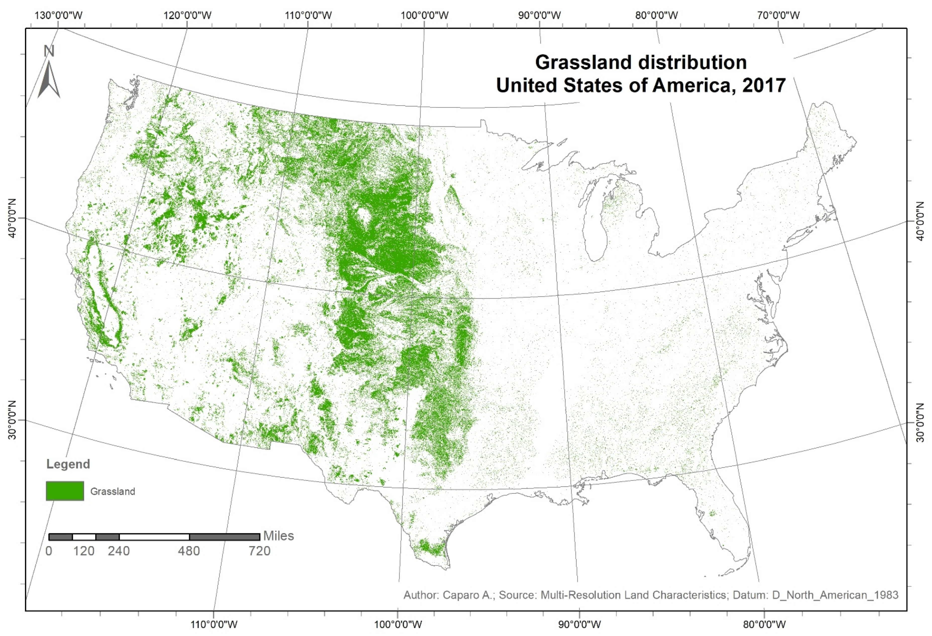
In 2017 in the U.S., there were an estimated 2.91 million km2 of grassland (Figure 1). The U.S. is the country with the second-largest area of grassland after China [54], sinking an estimated 13 teragrams of carbon (Tg C) annually [55]. According to Hufkens et al. [12], grasslands in North America are projected to increase 18% in spatial extent by 2100.
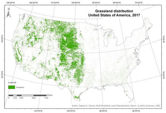
Figure 1.
Grassland distribution in contiguous United States of America (Data source: [14]).
Grasslands show highly dynamic growth that can vary over time and be affected by external factors [15]. Grasslands respond quickly in greening and physiological activity in response to climate drivers, especially precipitation and water availability [13,56] and, to a lesser extent, temperature [57]. Grassland productivity in the Great Plains is controlled by summer and spring precipitation [58].
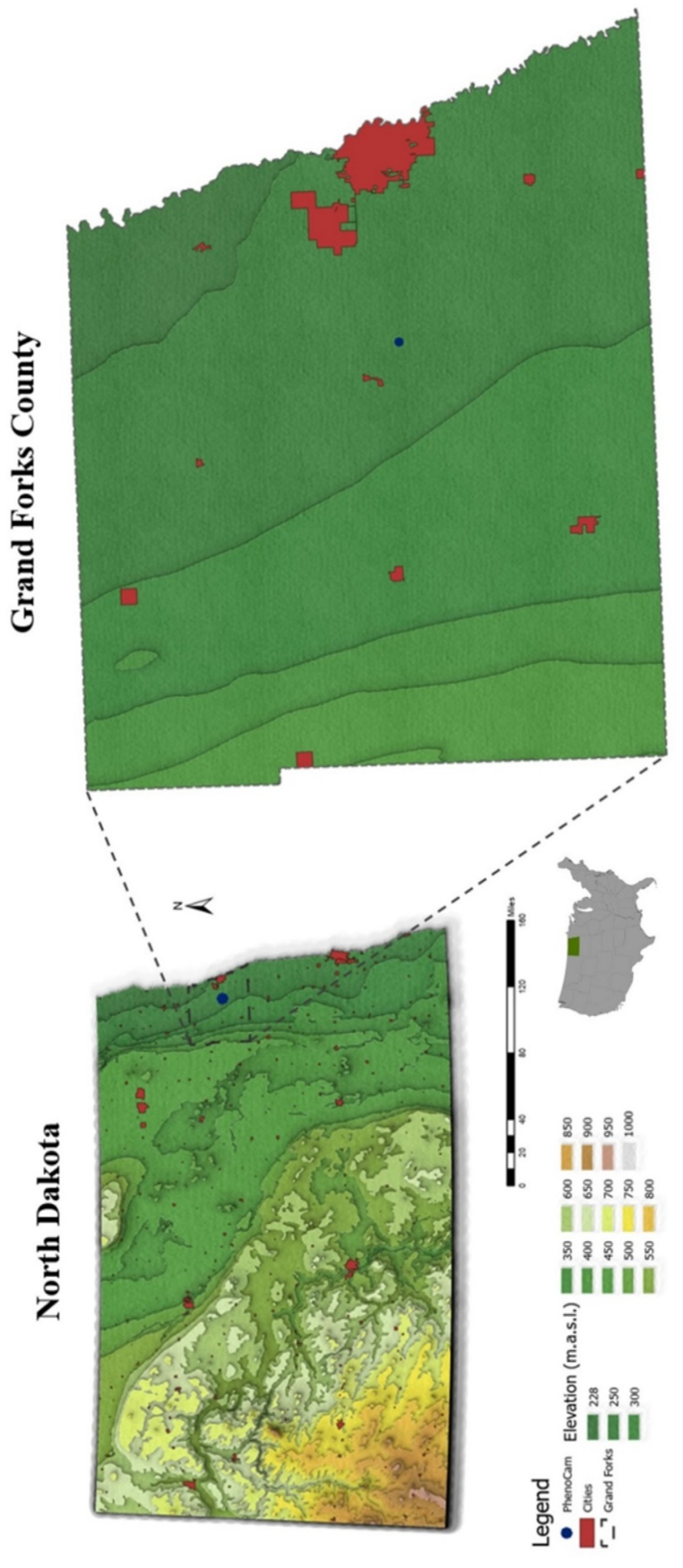
Our study site is located in Grand Forks County, one of 53 counties in the State of North Dakota, part of the Northern Great Plains region that shares the U.S. portion of the Red River Valley of the North with Minnesota (Figure 2). UND’s Oakville is an important area for tallgrass prairie research located 19 kilometers west of Grand Forks [59]. Oakville hosts one of the near-surface cameras of the PhenoCam Network [60].
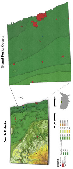
Figure 2.
Area of study. Grand Forks County, North Dakota. Red areas are towns and cities; blue dot shows PhenoCam at the Oakville location. The City of Grand Forks is the largest city in Grand Forks County, located on the eastern border with Minnesota. (Data Source: [61]).
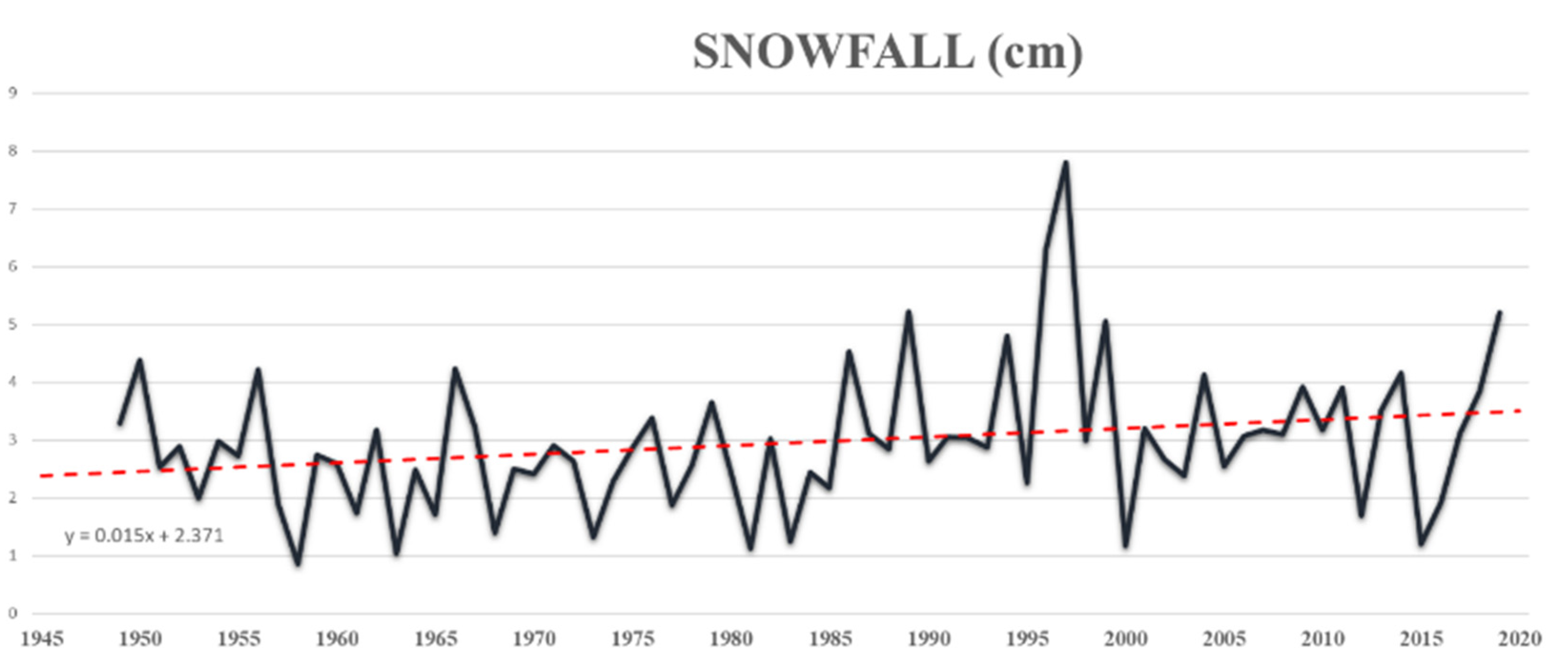
The climate of Grand Forks County is classified as Snow climate (D) fully humid (f) with warm summer (b), according to the updated Köppen–Geger climate classification [62]. Grand Forks’ coldest month is January, and the warmest is July. The county typically receives snow from October to May (Table 1). Snowfall is also highly variable among years but exhibits an average trend of increasing amounts (Figure 3).

Table 1.
Monthly average snowfall and temperature range in Grand Forks. (Data source: [63]).
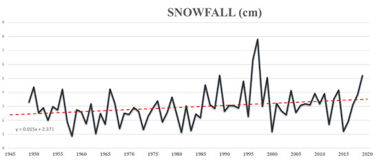
Figure 3.
Average daily snowfall by water year for Grand Forks (Data source: [64]).
Other important weather events in Grand Forks County are blizzards, defined as storms with wind speeds equal to or higher than 15.6 m/s [65]. During a period of 39 years (1979–2018), 100 blizzards were reported at the Grand Forks National Weather Service Forecast Office [64]. In North Dakota, the probability of a blizzard occurring annually is more than 50%, or more than one event every other year [66]. In the Red River Valley, the probability per year increases to between 61.6% to 76.4%, the highest in the U.S. [67].
4. Materials and Methods
Oblique terrestrial images have been widely used for monitoring the phenology of plants and snow cover. This section describes the steps followed to create an algorithm for estimating FSC in grasslands from a PhenoCam on flat terrain in eastern North Dakota. The workflow and accuracy assessment of the algorithm are also described.
4.1. Data
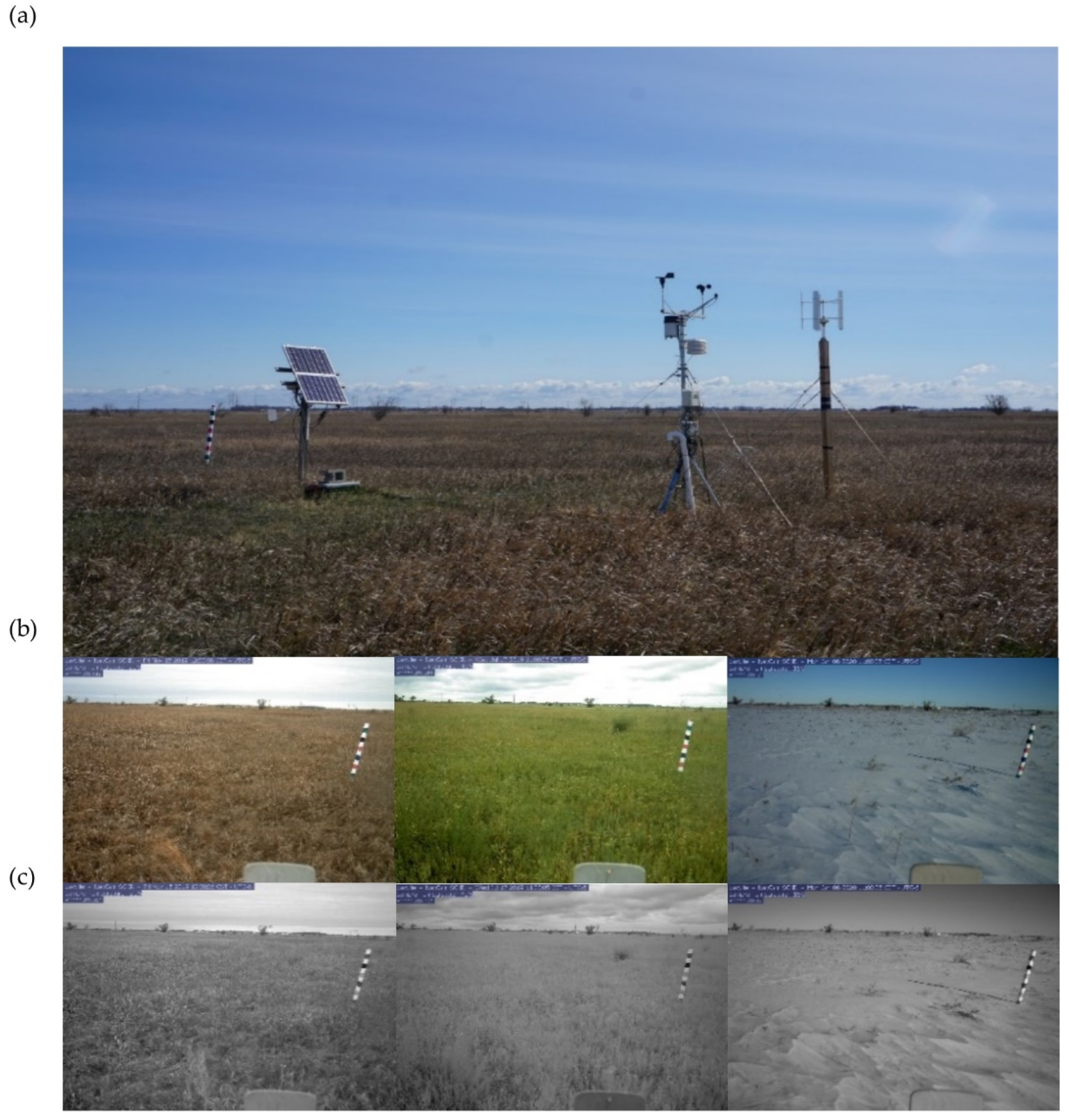
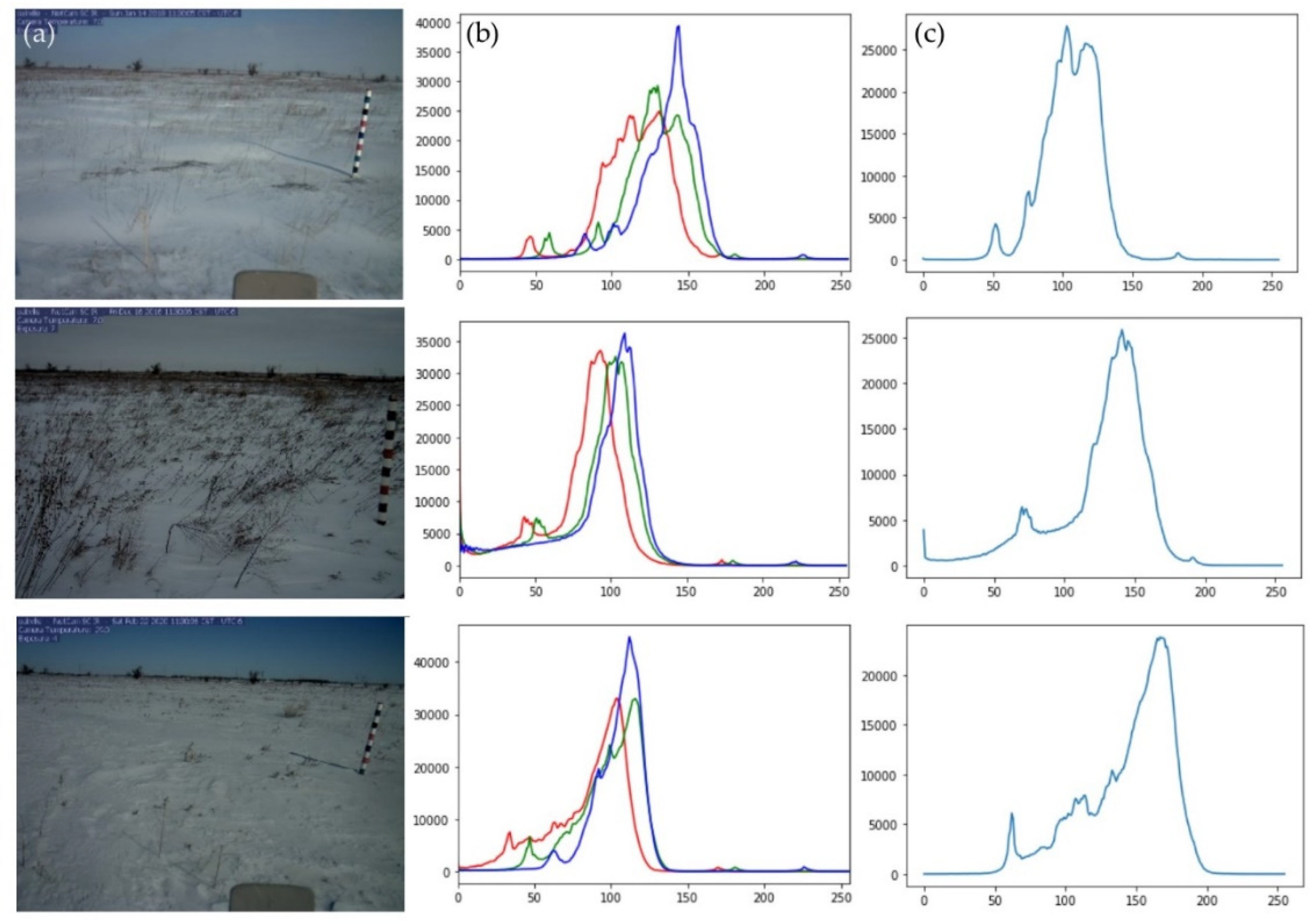
The PhenoCam in Oakville (Figure 4) is a Type I (highest quality camera among the PhenoCam Network). The StarDot NetCam SC has a 5-megapixel resolution and records images every 30 min between 04:00 and 23:30 LST [60]. There are two types of images: (1) the Red, Green and Blue (RGB) image, and (2) the monochrome RGB + Near-Infrared (MoNIR) (Figure 4). Both types are taken by the PhenoCam every 30 min at nearly the same time. The entire archive of images for the Oakville Prairie, as well as all other PhenoCam Network sites, are available online free of cost (for Oakville, see: https://phenocam.sr.unh.edu/webcam/sites/oakville/ accessed on 15 May 2021).

Figure 4.
(a) Research site at the Oakville Prairie Biology Field Station, including the PhenoCam; (b) example RGB images; and (c) example MoNIR images through the year acquired by the PhenoCam.
For each of the five winter seasons we studied (01 October to 30 April 2015–2016 to 2019–2020) we selected one PhenoCam image per day acquired between 10:30 a.m. and 12:30 p.m. LST to reduce solar illumination variations during the months that show snow presence. The majority of those we used were taken at 11:30 a.m. LST. A total of 1712 images were downloaded: 856 RGB images and the corresponding 856 MoNIR images.
4.2. Validation of Optimal Band Selection Scenario for FSC Estimation
Previous work used the Blue band to calculate FSC. For example, [46] applied a threshold in the first local minimum above 127 in the Blue band histogram to map snow cover. In addition, they selected the Blue band after processing the three bands separately and got similar values. We also explored the utility of the MoNIR band for FSC calculation.
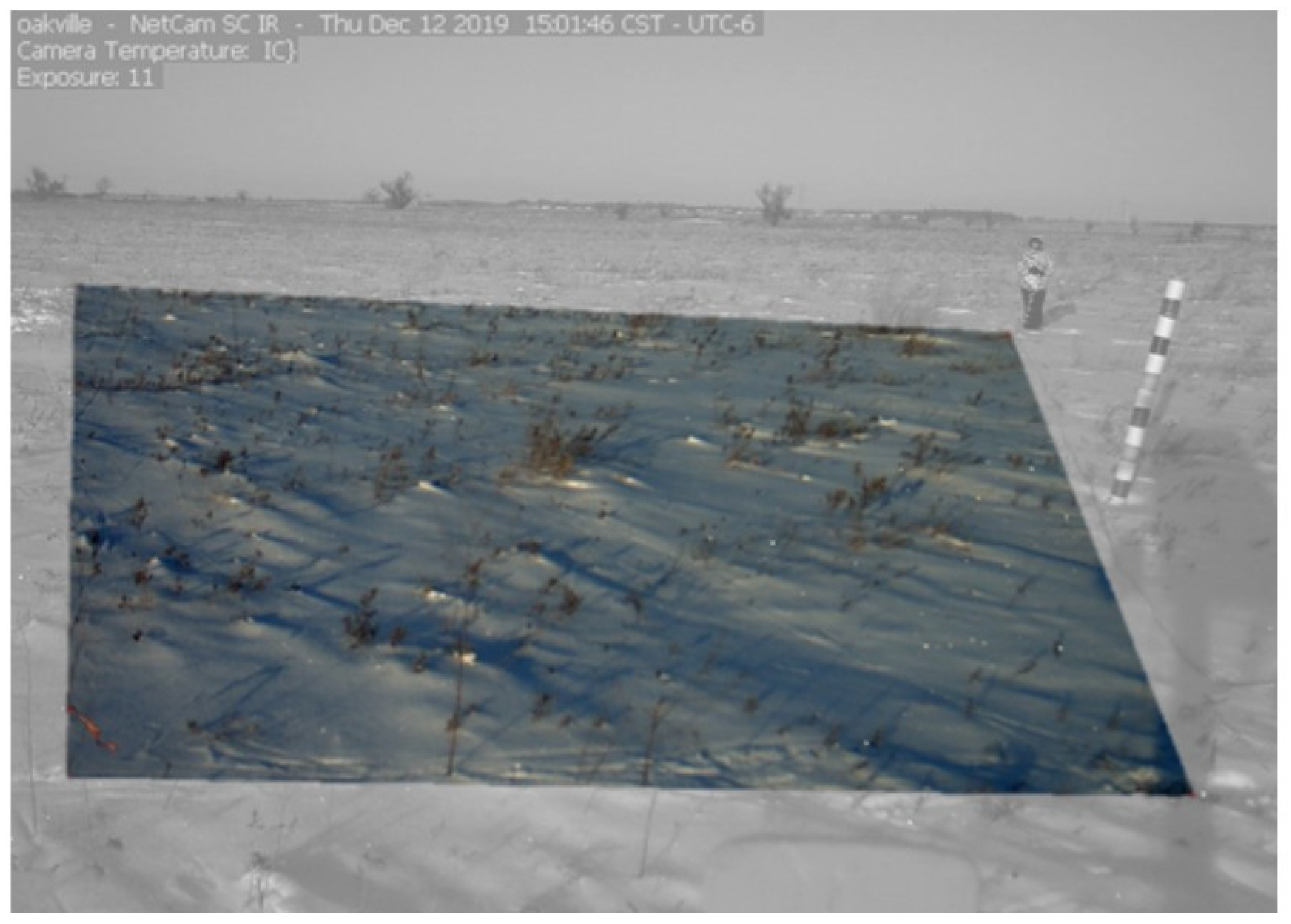
To select images that contained some snow cover, we calculated the average brightness of each band for all the images we downloaded. The oblique images from Oakville usually have a panel, a pole, information (name, date, and hour), and the sky (Figure 5), all of which we excluded from the band brightness calculations. Calculating average brightness for each band for all images allowed us to understand which PhenoCam bands were most affected by the presence of snow cover.
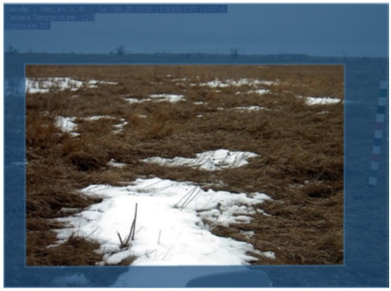
Figure 5.
Example PhenoCam image showing the area used to calculate FSC in each band.
Guided by our band brightness calculations, 38 images were selected from the entire dataset, representing 11 categories of FSC (0%, 10%, 20%, 30%, 40%, 50%, 60%, 70%, 80%, 90%, and 100%) for four periods (the winter seasons of 2015–2016, 2016–2017, 2017–2018, and 2018–2019). Three images with sastrugi present were also selected. We tested the images for calculating the FSC in four different scenarios:
Scenario 1: Blue band threshold
In the first scenario, pixels with Digital Numbers (DNs) greater than or equal to 127 in the Blue band were classified as “snow”, and pixels with lower Blue DNs were classified as “no-Snow” [46].
Scenario 2: Monochromatic RGB+NIR (MoNIR) threshold
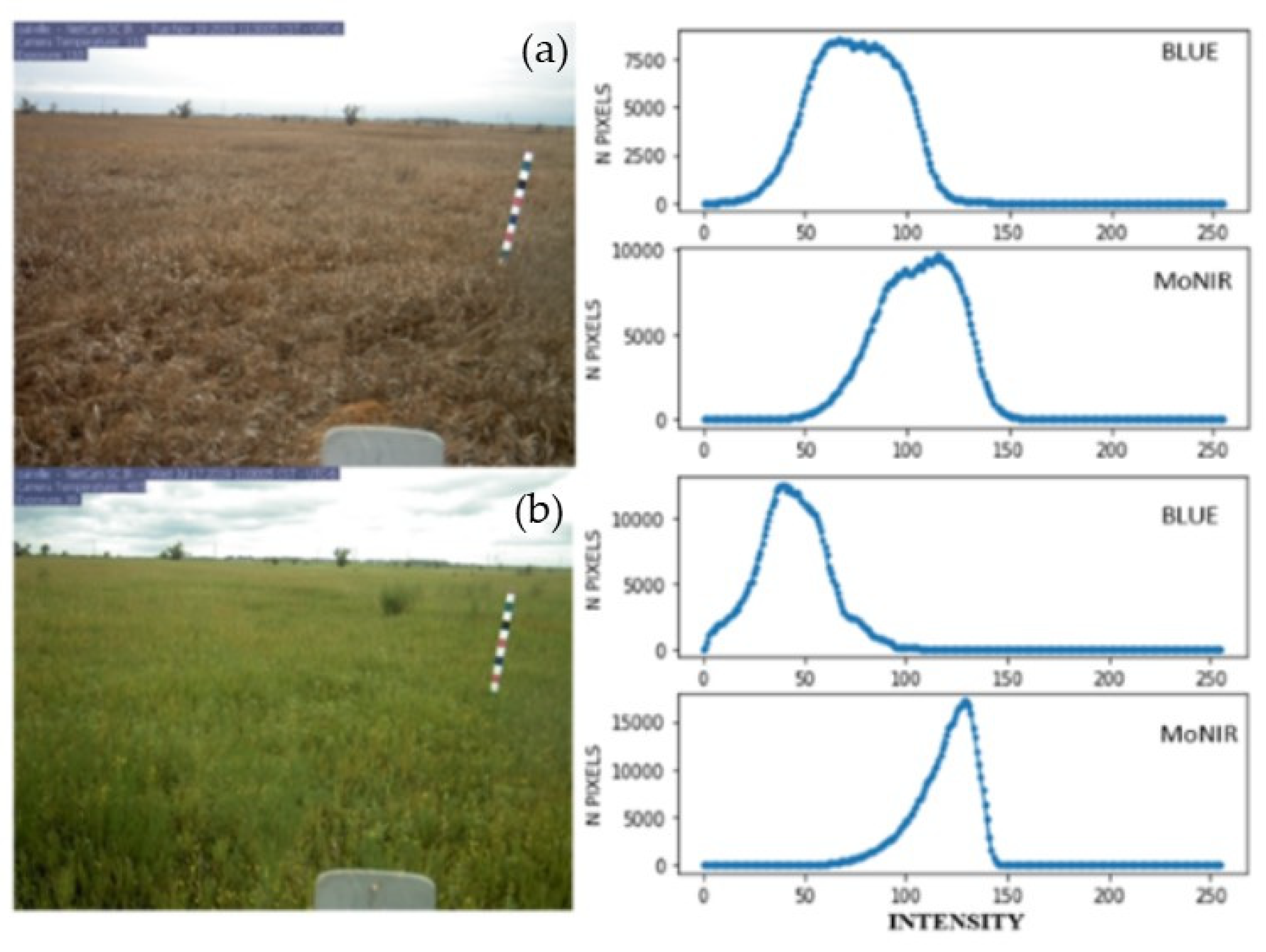
The second scenario selected as snow all pixels with DNs greater than or equal to 127 in the MoNIR band. Depending on the land cover and the sunlight, the reflectance value may show differences for each band histogram (Figure 6).

Figure 6.
(a) Senesced grassland, (b) Green grassland and their corresponding Blue and MoNIR band histograms.
Because shadowing on snow cover has been shown to confound efforts to calculate FSC from PhenoCam data, we developed two additional scenarios. The third and fourth scenarios, then, exploited the relationship between MoNIR and the Blue band calculated by:
The resulting DNs considered shadow on snow cover fell between −80 and 20. These were selected and used in the next two scenarios.
Scenario 3: Blue (B) band threshold + Shadow
The selected values from Shadow were added to the Blue band selected pixels from the first scenario.
Scenario 4: MoNIR + Shadow
The fourth scenario added the pixels from shadow to the pixels from scenario two.
To validate which scenario worked best for each FSC, we used the Accuracy Assessment tool in ArcGIS 10.6, which generates points for each class. For this study, we generated 50 points per image, 25 for each class (snow or no snow). Then, we visually compared the selected points to the original image to generate a confusion matrix between both classes.
4.3. Region of Interest (ROI)
We used the same area (ROI) on all downloaded PhenoCam images to calculate FSC. The ROI was delimited and measured in the field, and the resulting polygon was captured and digitized. The area of the polygon was calculated using Heron’s Area formula [68]. The ROI has a real-world area of 141.45 m2, and its equivalent image area is 521,898 u2 (pixels) (Figure 7).
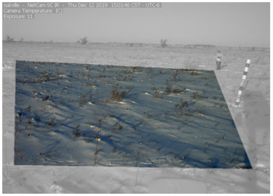
Figure 7.
Region of Interest (ROI). Note the shadowing on the snow cover.
4.4. FSC Algorithm
We developed our FSC algorithm using the Python 3 programming language. The installation of three modules was required: OpenCV, Matplotlib, and URLLIB.
First, the script we developed asks the user to enter the URL of the PhenoCam image to be processed, which allows the user to select the best image each day for FSC estimation. Then, both images, the RGB and MoNIR, are downloaded, and the processing starts. Each band is isolated, and the average DN is calculated. The averages of the Red, Green, and Blue images are also calculated.
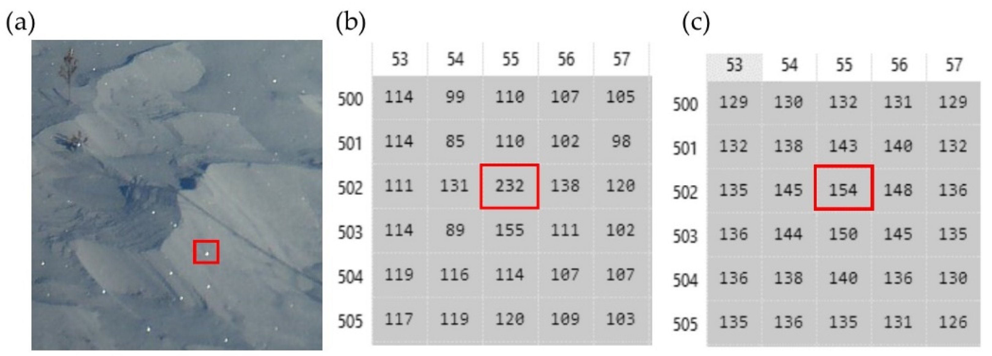
The Blue and MoNIR bands were normalized, and a Gaussian filter with an intensity of five is applied to their histograms. The Gaussian filter smooths the histogram curve by averaging pixels (5 × 5); this process helps to correct high or low values considered as noise (Figure 8).

Figure 8.
(a) Image with noise, (b) pixel values before and (c) after the Gaussian Filter.
The Blue and MoNIR bands are used to calculate the shadow part of the image. The values between −80 and 20 are considered shadow. The next steps are based on decisions that the algorithm takes using knowledge from validation of the scenarios described. The workflow, also shown in Figure 9, is:
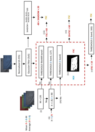
Figure 9.
Image processing workflow.
- Images with a MoNIR average (M) greater than 135 are classified using the MoNIR band. The threshold value is the lowest between RGB average, M and 100.
- The Red band has higher values when there is no snow and the lowest values with snow presence, and this is inverse with the Blue band. A ratio between B/R is calculated. When the value is lower than one and B is lower than 90, a threshold of 127 is applied to the Blue band.
- When i and ii are false, a threshold is applied to the Blue band, whose value is the lowest among RGB average, Blue and 100.
- Steps i–iii produce an image with values of 0 (no snow) or 1 (snow). The new image is masked with the region of interest (ROI), and the FSC is calculated.
- Sometimes, grassland has reflectance values as high as snow reflectance values. When the FSC value is lower than 10, the FSC is recalculated using a higher threshold value of 165.
- Images with FSC between 10 and 60 do not have to pass to any other classification.
- The values calculated with the shadow formula are added to the images with FSC higher than 60, which is the final FSC value.
Finally, the FSC is saved with the name of the image as a text file.
4.5. FSC Algorithm Accuracy Assessment
The accuracy of the algorithm was calculated using the root-mean-squared-error (RMSE), which compared the estimated FSC values with FSC values determined by two specialists in image interpretation [42]. The RMSE was calculated with the following formula:
The RMSE was calculated for two periods: 2017–2018 and 2018–2019 in both cases from 1 October to 30 April. The first period has a total of 177 images, and the second period 92 images. All the classified images were acquired at 11:30 LST except for two images with fog, which were changed to images acquired at 12:00 and 12:30 LST of the same day after the fog had lifted.
Gathering observed FSC values required help from visual image interpretation and PhenoCam experts outside the study. Both experts visually estimated FSC over the entire ground surface imaged, and not just within the ROI, for the winters of 2017–2018 and 2018–2019. The visual estimates of FSC were provided as values between 0% and 100%. It is important to mention the experts were instructed to estimate FSC at 10% intervals (0%, 10%, 20%...100%).
In addition, we selected two images for each of the five winters we studied (10 images total) to validate the classification. The selected images had an FSC estimated by our algorithm at between 40% and 60%. On each selected image, we randomly selected 50 points per class (two classes, “snow” vs. “no snow”; 100 points per image), resulting in 1,000 validation points. For each validation point, we visually compared the snow/no-snow result with the corresponding pixel from each PhenoCam source image, noting when our algorithm correctly and incorrectly identified “snow” or “no snow” pixels [40].
5. Results
Red and Blue reflectances are highly variable because of snow presence. When the ROI is 0% snow covered, it is 100% covered by grassland. The Red band had higher values when the images show vegetation and lower when there is snow present. This is in contrast to the Blue band that had lower values when there was no snow (Figure 10).
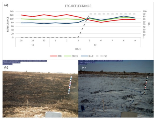
Figure 10.
(a) Band reflectance variation, (b) picture without snow presence and (c) with snow presence in Oakville.
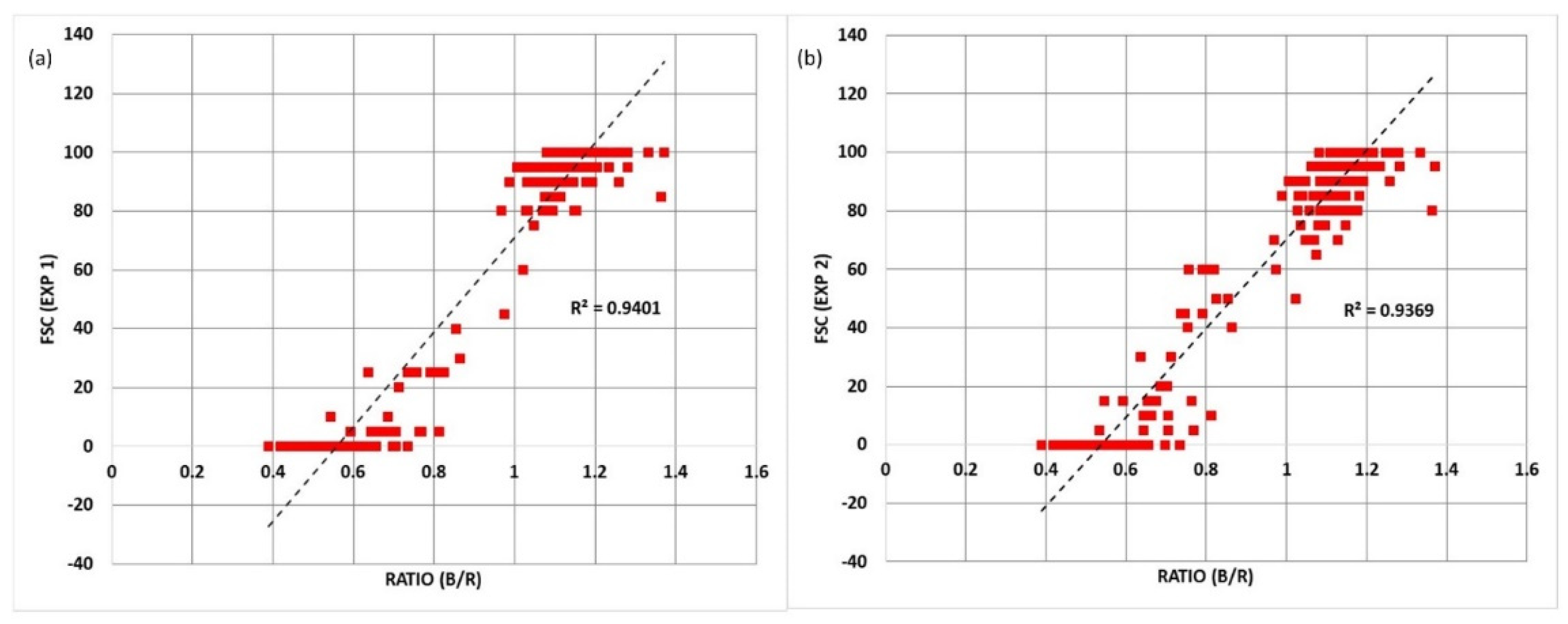
The Red and Blue bands had different behaviors when there was no snow, but with snow present, they had similar curves. We assumed that the ratio (B/R) could be used to differentiate between snow and no-snow and used different threshold values in the Blue band image. The ratio was compared with the experts’ FSC estimations. Figure 11 shows that in both cases, the R2 was higher than 0.9, showing a strong relation between them. In most of the cases, when FSC = 0, the ratio value was lower than 1.0.
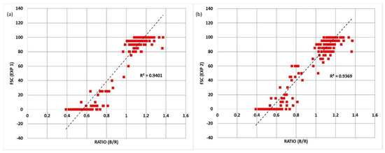
Figure 11.
Ratio (B/R) against FSC estimated by (a) Expert 1 and (b) Expert 2.
5.1. Validation of Optimal Band Selection Scenario for FSC Estimation
The Blue band yielded accurate results when FSC is between 0% and 20%. Grassland presence was reflected in the low Blue band amount. Between 60% and 100%, MoNIR + shadow had higher accuracy values, but they were not as high as expected. In the algorithm, we decided to apply shadow when the FSC was greater than 60% because that was when it showed better accuracy.
Pixel misclassification was caused by many factors. At the beginning of the season, grassland reflectance values were high in the Red and MoNIR bands. During snow presence, there was no constancy in the level of brightness. When it was bright, there were more shadow areas, and MoNIR and the Blue band had different behaviors. Sastrugi also caused misclassification because of the different shadows that it produced. Table 2 summarizes the accuracy of the 44 images.

Table 2.
Accuracy obtained in the four scenarios for different FSC values.
5.2. FSC Algorithm Accuracy Assessment
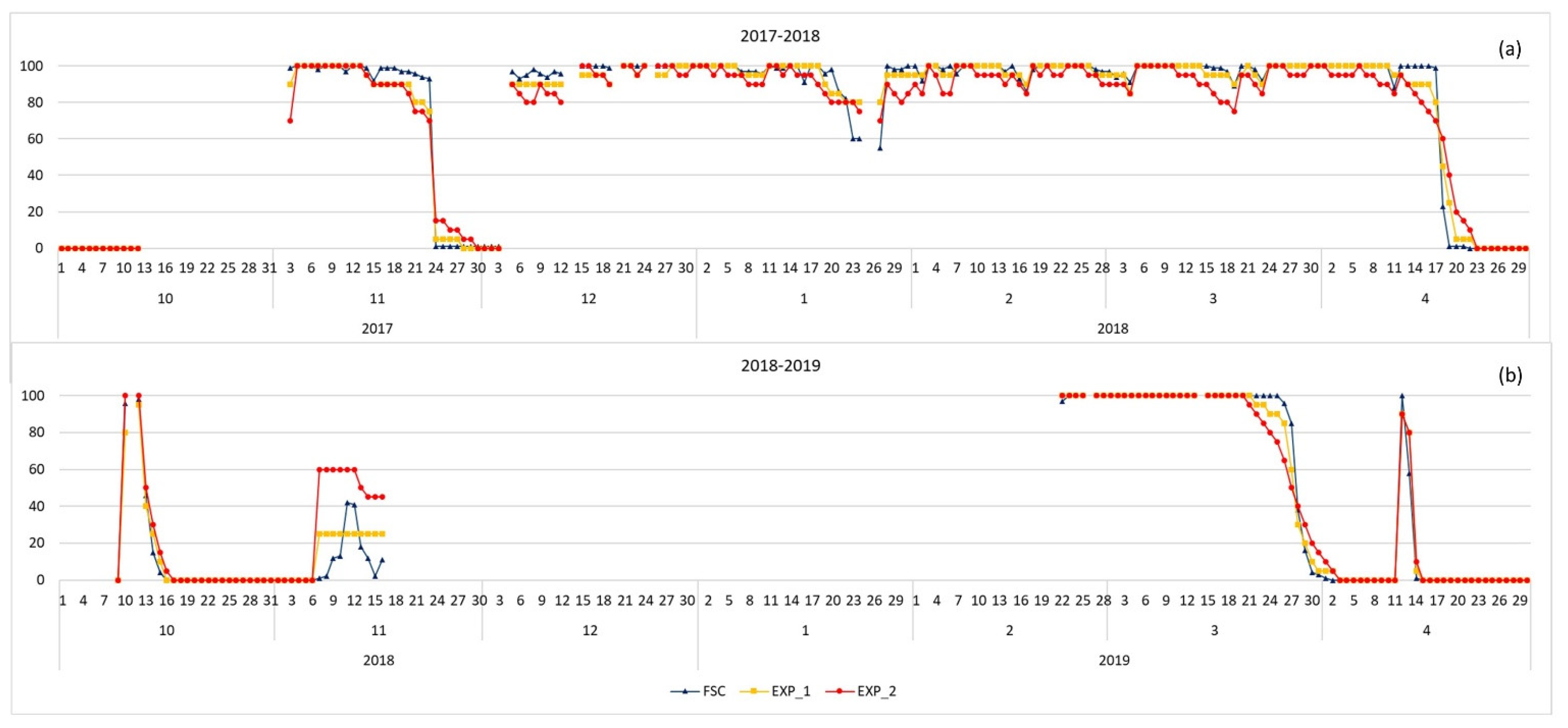
A total of 288 processed images were compared with visual estimations. These images are part of the winter of 2017–2018 and 2018–2019. For the first winter, 184 images were processed, and a Root Mean Square Error (RMSE) of 3.43% and 6.66% FSC were obtained, compared with Expert 1 and Expert 2, respectively. The second winter had 104 images, and the RMSEs were 7.01% and 14.71% FSC (Table 3). The estimated FSC was closer to the experts’ values, as they both had similar curves (Figure 12). Our pixel-based accuracy assessment showed that the overall accuracy of the images selected for validation was 92%.

Table 3.
RMSE for the FSC algorithm.

Figure 12.
Algorithm-derived FSC estimation comparison with estimated FSC values by two visual image interpretation experts (EXP_1 and EXP_2) over (a) winter 2017–2018 and (b) winter 2018–2019.
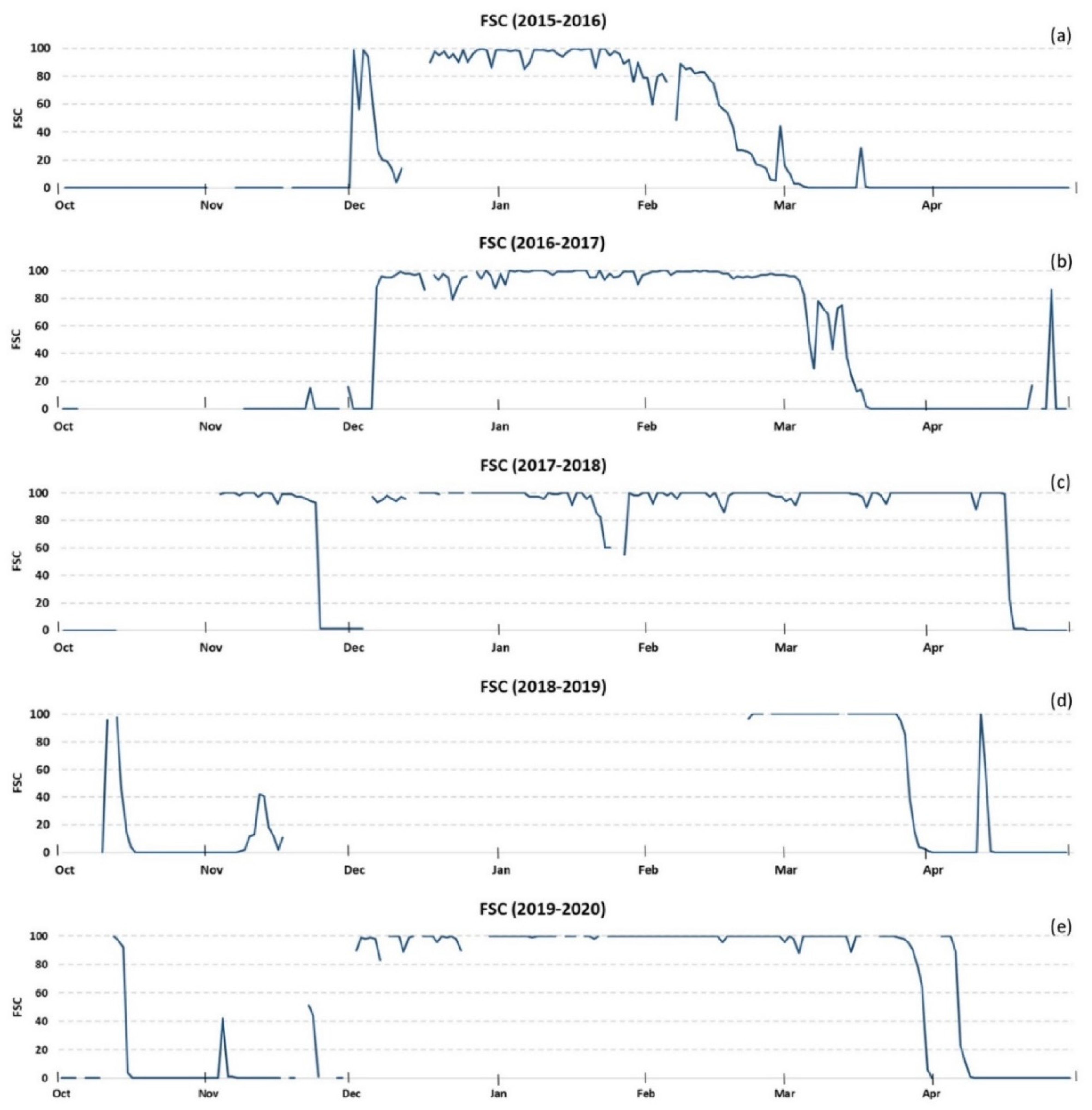
Figure 13 shows the five years of the estimated FSC from our PhenoCam. There was no distinct pattern in FSC in Oakville. Except for the winter of 2017–2018, the majority of winters showed snowfall events at the beginning and at the end that remained for a couple of days, followed by rapid snow melting.
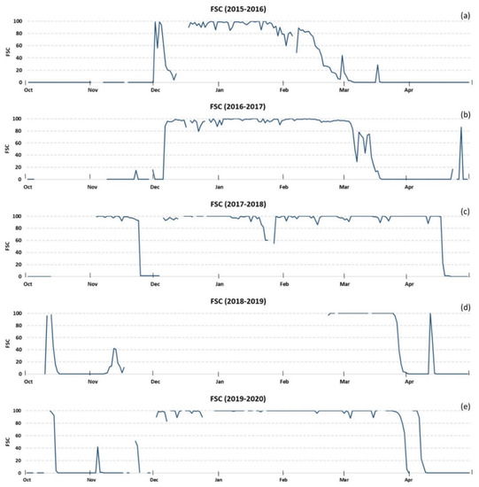
Figure 13.
FSC for the winters of (a) 2015–2016, (b) 2016–2017, (c) 2017–2018, (d) 2018–2019 and (e) 2019–2020 in Oakville. Blank spaces on the graphs related to periods of missing data (the camera did not operate or there were no suitable images).
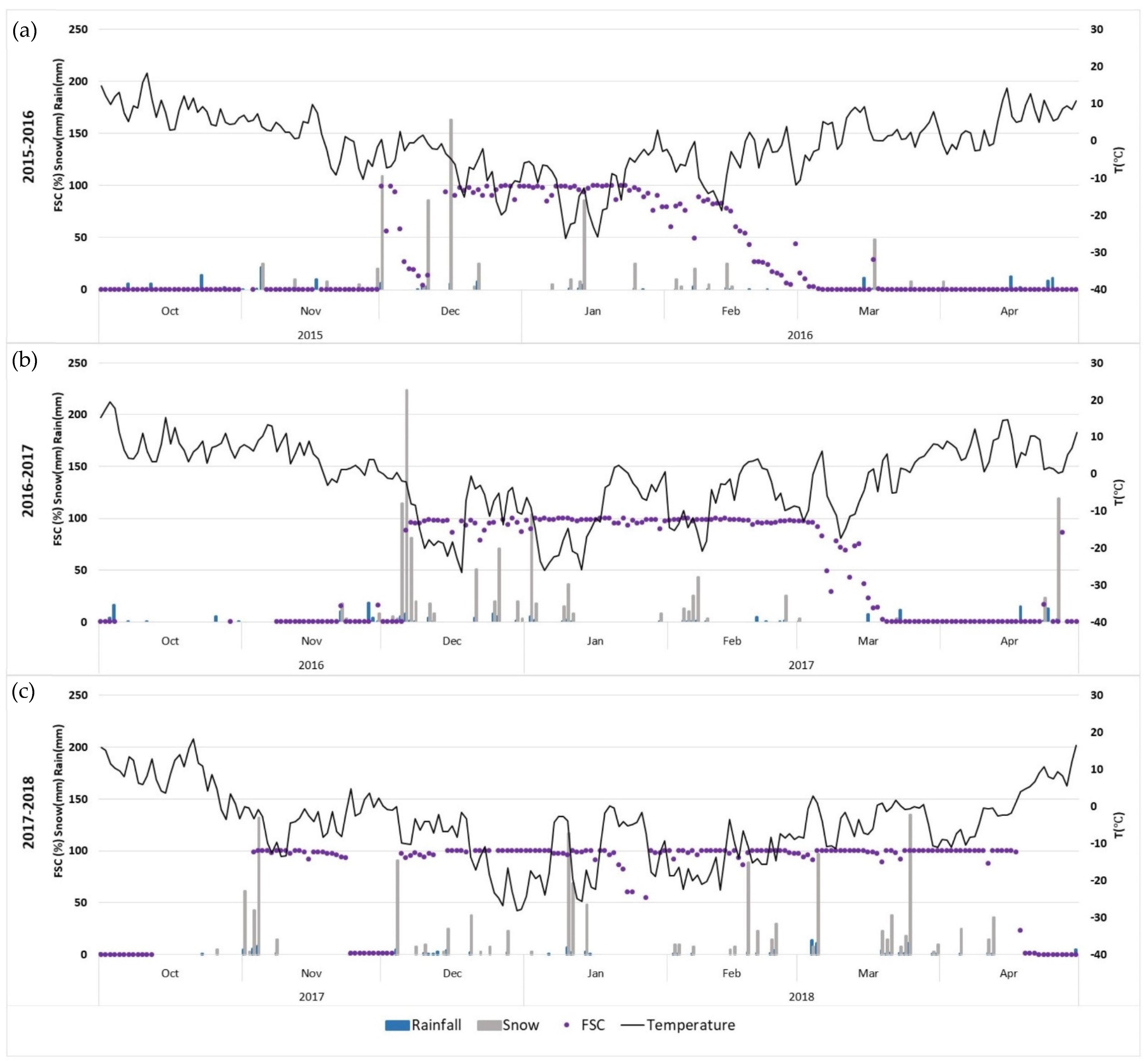
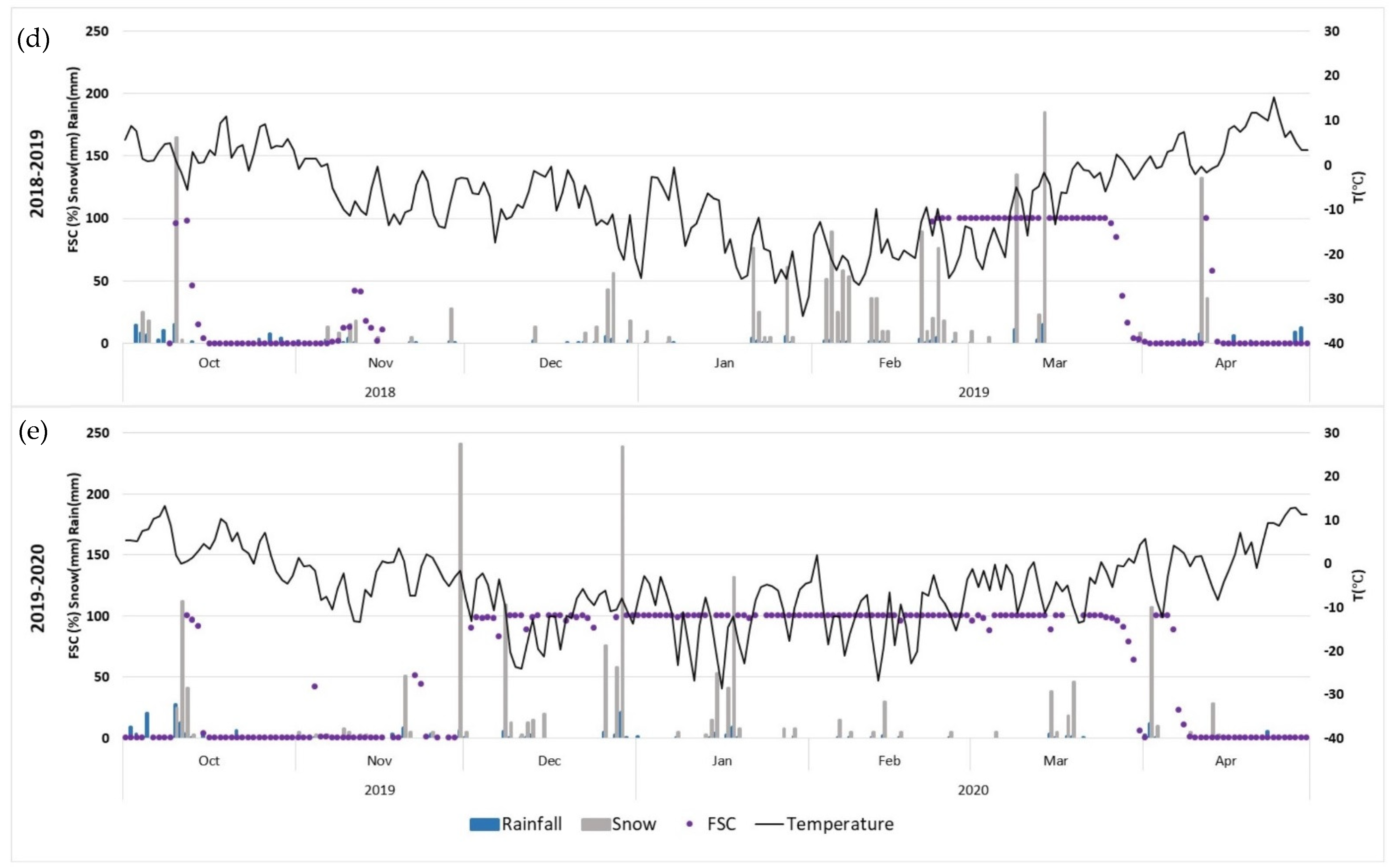
During the winter of 2015–2016, 203 days were evaluated. The first snow was 1 December, and for 91 days, there was greater than 1% FSC, and 110 days had an FSC of 0. The last snowfall event was on 17 March. The winter of 2016–2017 had 175 images. The first snow was 22 November and the next 102 days had snow present. At the end of the season, two snowfall events occurred on 23 and 27 April. The winter of 2017–2018 had 184 images. This winter was different from the other winters in the study period because it had two snow periods, as was common in other regions (e.g. [69]). The first period was from 3 November to 23 November. Then, the snow melted for 10 days, and on 5 December, Oakville was again covered by snow for 132 consecutive days before it took just three days to melt entirely. The winter of 2018–2019 had one snowfall at the beginning and one at the end of the season. For this winter, a total of 104 images were processed. The first snowfall was 10 October then, it melted, and the next event was after 22 days. The snow melted on 1 April, but there were two days with snow cover on 12 and 13 April. The winter of 2019–2020 has 190 images. This period had 64 snow-free days and three snowfall events before it was covered with snow for 110 consecutive days. At the end of the season, on 3 April, a snowfall remained on the grassland for seven days. Figure 14 and Figure 15 show the obtained FSC compared with temperature, snowfall, and rainfall for the study period [63].
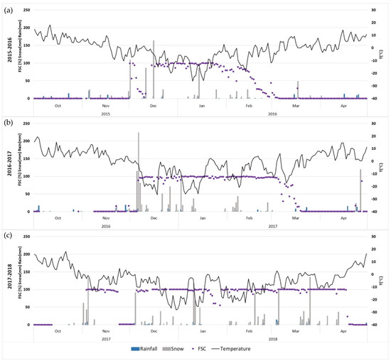
Figure 14.
FSC, temperature, snowfall, and rainfall for the winters of (a) 2015–2016, (b) 2016–2017 and (c) 2017–2018 in Oakville.
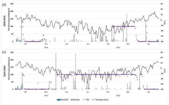
Figure 15.
FSC, temperature, snowfall, and rainfall for the winters of (d) 2018–2019 and (e) 2019–2020 in Oakville.
6. Discussion
We presented a semi-automatic procedure to obtain the FSC in grassland cover, highlighting the potential of the PhenoCam in Oakville. All the findings were exclusive for our grassland cover and for winter weather conditions. Despite the use of just the Blue band in previous research, we focused on the other spectral bands that could improve the FSC estimation. Assuming that there is no change in elevation, we also did not use a Digital Elevation Model (DEM) to georeference the image and calculate the total area.
One of the main reasons for the need for this high temporal resolution data is the variability of snow cover. It takes one day to go from 0 to 100 FSC and sometimes less than five days for snow to completely melt (Figure 16).

Figure 16.
Snow melting and its respective FSC in Oakville. (a) FSC = 100%, date: 12 October 2019; (b) FSC = 97%, date: 13 October 2019; (c) FSC = 94%, date: 14 October 2019; (d) FSC = 4%, date: 15 October 2019 and (e) FSC= 0, date: 16 October 2019.
Other studies have used the Blue band because the three bands have similar behaviors in mountainous regions [19]. Figure 17 shows that in separate cases of 100% FSC, the three bands have different histograms that could be related to sunlight. We highlighted that previous studies did not have MoNIR band, and implementing it in our study allowed us to have fewer cases of misclassification because of shadows.
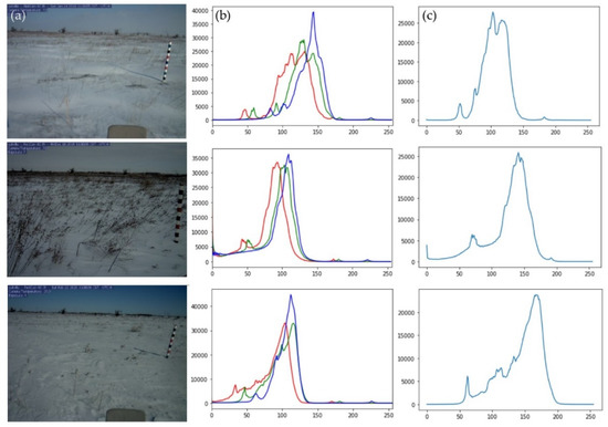
Figure 17.
(a) Snow cover in Oakville. (b) Red-Green-Blue bands histograms and (c) MoNIR band histogram.
Furthermore, previous studies have used 127 as the minimum value in the Blue band because they found that areas with snow cover in this band have a value greater or equal to 127. In this research, we used the Blue/MoNIR average, and if these values were greater than 100, the threshold value was set at 100. Figure 18 shows that in this region, the Blue band value, when there is snow present, was greater than 80. The difference between these values shows that depending on the region (mountainous or a valley) and the land cover (forest, grassland, etc.), the Blue band will have different behavior.
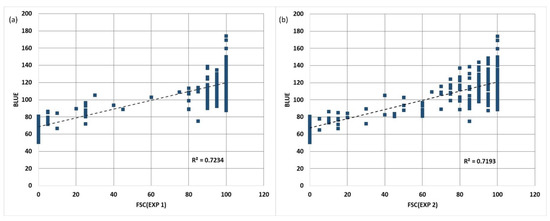
Figure 18.
Blue band value compared with (a) Expert 1 and (b) Expert 2 FSC values.
One of the biggest issues related to the FSC from near-surface remote sensing is shadows. These can create misclassifications and significantly decrease accuracy. The use of the MoNIR band helps to improve the classification (Figure 19).
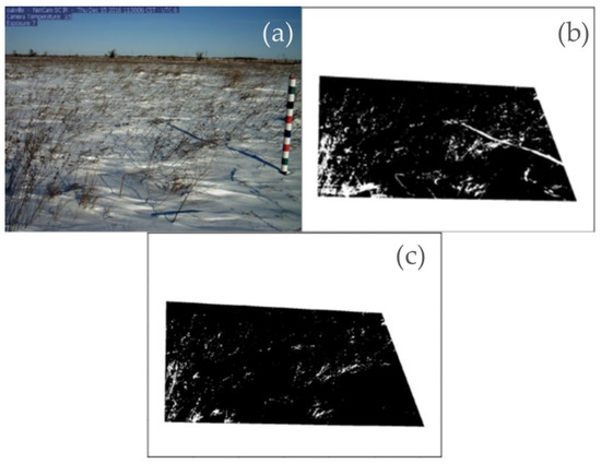
Figure 19.
(a) Image in RGB, (b) FSC with shadow misclassification and (c) FSC adding the shadow pixels.
7. Conclusions
This research used PhenoCam images in a semi-automatic way to estimate FSC at a site within Oakville, showing that the capabilities of the images are not only limited to monitor vegetation phenology. The results validated with two experts had average RMSEs of 5.02% and 10.32%. Our pixel-based accuracy assessment showed that the overall accuracy of the images selected for validation was 92%. The number of cameras of the PhenoCam Network makes it possible to provide localized FSC estimates over the entire country, generating a database that can be used to validate and complement satellite data.
Most of the images are classified using the Blue band, but thanks to the MoNIR band, the algorithm recognizes darker areas (shadows), and also, some days when the Blue band has a low reflectance value, the MoNIR band showed that it could be used to classify snow cover. Not all the cameras in the PhenoCam Network include the MoNIR band, and these sites could use the Blue band to estimate the FSC.
During the study period (2015–2020), there was not a consistent pattern in the FSC in this area. Some years the first snowfall was on 1 December and other years it was on 9 October. The same happened with the snowmelt; in 2016, the last day with snow present was in March, while other years had their last snowfall in April. FSC is a parameter that depends on snowfall, temperature, energy flux, and their anomalies.
Some limitations of this research were the field of view, the oblique view, and the vignetting effect; all of these related to the sensor. The field of view, which determines the area in the image, compared with other sensors, was small. The oblique view generates pixels that represent different real sizes; the closer the pixel, the smaller the area of ground represented. Vignetting happens when the borders of the image have darker colors compared with the center of the image.
A significant limitation was the subjectivity introduced into the accuracy assessment because we relied on the visual estimates of FSC made by two experts. Although we generally followed the accuracy assessment methods described by other research [50], we also added a pixel-based assessment, following methods described by [41]. In future studies, our goal is to tie our PhenoCam observations to corresponding data gathered by satellite sensors. We support the idea that datasets should be combined to achieve higher quality and less uncertainty in the remote sensing of snow cover [70].
Other limitations are external factors like weather conditions, land cover, and the presence of objects out of the study. On a sunny day, the scene is brighter, but there are also more shadows, and on cloudy days, the images have relatively low contrast. Blizzards and fog decrease visibility, and strong winds generate sastrugi. The land cover at Oakville is grassland, which during the senescence period has a golden color and sometimes is as bright as snow, creating misclassification.
FSC is an important parameter that has to be monitored. The use of PhenoCam images and Python language, both free, allow researchers to keep developing scripts and to improve the existing work. This research was focused on one grassland site; future work should explore extending the findings to additional PhenoCam Network sites, working with other land covers and at different latitudes. Furthermore, future work should include the relationship between FSC and other parameters, such as positive and negative feedbacks related to climate change, the beginning and end of the growing season, and soil temperature and moisture.
Author Contributions
Data curation, A.C.B.; Formal analysis, A.C.B.; Methodology, A.C.B. and B.C.R.; Supervision, B.C.R.; Writing—original draft, A.C.B.; Writing—review & editing, B.C.R. All authors have read and agreed to the published version of the manuscript.
Funding
This work was supported by the AmericaView program by the U.S. Geological Survey under Grant/Cooperative Agreement No. G18AP00077. The UND Field Station Committee also funded the mobile data connection to transfer data from the Oakville PhenoCam to the PhenoCamNetwork at the University of New Hampshire.
Acknowledgments
We acknowledge Paul E. Todhunter, Jeffrey A. VanLooy, Morgen Burke, Earl Klug, and the Department of Geography and Geographic Information Science at UND for their support of this research.
Conflicts of Interest
The authors declare no conflict of interest. The funders had no role in the design of the study; in the collection, analyses, or interpretation of data; in the writing of the manuscript, or in the decision to publish the results.
This manuscript highlights the main findings of an M.S. thesis in Geography at UND, which has been published in UND’s digital repository at https://commons.und.edu/theses/3260/ accessed on 15 May 2021.
References
- Parry, M.L.; Canziani, O.F.; Palutikof, J.P.; van der Linden, P.J.; Hanson, C.E. Climate Change 2007: Impacts, Adaptation and Vulnerability. Contribution of Working Group II to the Fourth Assessment Report of the Intergovernmental Panel on Climate Change; Cambridge University Press: Cambridge, UK, 2007; p. 976. [Google Scholar]
- Reed, B.C.; Schwartz, M.D.; Xiao, X. Remote sensing phenology. In Phenology of Ecosystem Processes; Springer: New York, NY, USA, 2009; pp. 231–246. [Google Scholar] [CrossRef]
- Gao, J. Quantification of grassland properties: How it can benefit from geoinformatic technologies? Int. J. Remote Sens. 2006, 27, 1351–1365. [Google Scholar] [CrossRef]
- Brown, T.B.; Hultine, K.R.; Steltzer, H.; Denny, E.G.; Denslow, M.W.; Granados, J.; Henderson, S.; Moore, D.; Nagai, S.; SanClements, M.; et al. Using phenocams to monitor our changing earth: Toward a global phenocam network. Front Ecol Environ 2016, 14, 84–93. [Google Scholar] [CrossRef]
- Browning, D.; Karl, J.; Morin, D.; Richardson, A.; Tweedie, C. Phenocams bridge the gap between field and satellite observations in an arid grassland ecosystem. Remote Sens. 2017, 9, 1071. [Google Scholar] [CrossRef]
- Richardson, A.D. Tracking seasonal rhythms of plants in diverse ecosystems with digital camera imagery. New Phytol. 2019, 222, 1742–1750. [Google Scholar] [CrossRef]
- Richardson, A.D.; Hufkens, K.; Milliman, T.; Aubrecht, D.M.; Chen, M.; Gray, J.M.; Johnston, M.R.; Keenan, T.F.; Klosterman, S.T.; Kosmala, M.; et al. Tracking vegetation phenology across diverse north american biomes using PhenoCam imagery. Sci. Data 2018, 5, 180028. [Google Scholar] [CrossRef] [PubMed]
- Richardson, A.; Klosterman, S.T.; Toomey, M. Near-surface sensor-derived phenology. In Phenology: An Integrative Environmental Science; Springer: Berlin/Heidelberg, Germany, 2013; pp. 413–430. [Google Scholar]
- Richardson, A.D.; Braswell, B.H.; Hollinger, D.Y.; Jenkins, J.P.; Ollinger, S.V. Nearsurface remote sensing of spatial and temporal variation in canopy phenology. Ecol. Appl. 2009, 19, 12. [Google Scholar] [CrossRef]
- Keenan, T.F.; Richardson, A.D.; Hufkens, K. On quantifying the apparent temperature sensitivity of plant phenology. New Phytol. 2020, 225, 1033–1040. [Google Scholar] [CrossRef]
- Zhou, Q.; Rover, J.; Brown, J.; Worstell, B.; Howard, D.; Wu, Z.; Gallant, A.; Rundquist, B.; Burke, M. Monitoring landscape dynamics in central, U.S. grasslands with harmonized Landsat-8 and Sentinel-2 time series data. Remote Sens. 2019, 11, 328. [Google Scholar] [CrossRef]
- Hufkens, K.; Keenan, T.F.; Flanagan, L.B.; Scott, R.L.; Bernacchi, C.J.; Joo, C.J.B.E.; Brunsell, N.A.; Verfaillie, J.; Richardson, K.H.A.D. Productivity of North American grasslands is increased under future climate scenarios despite rising aridity. Nat. Clim. Chang. 2016, 6, 710–714. [Google Scholar] [CrossRef]
- Migliavacca, M.; Galvagno, M.; Cremonese, E.; Rossini, M.; Meroni, M.; Sonnentag, O.; Cogliati, S.; Manca, G.; Diotri, F.; Busetto, L.; et al. Using digital repeat photography and Eddy Covariance data to model grassland phenology and photosynthetic CO2 uptake. Agric. For. Meteorol. 2011, 151, 1325–1337. [Google Scholar] [CrossRef]
- Multi-Resolution Land Characteristics. Available online: https://www.mrlc.gov/ (accessed on 20 December 2019).
- Ali, I.; Cawkwell, F.; Dwyer, E.; Barrett, B.; Green, S. Satellite remote sensing of grasslands: From observation to management. J. Plant Ecol. 2016, 9, 649–671. [Google Scholar] [CrossRef]
- Seyednasrollah, B.; Young, A.M.; Hufkens, K.; Milliman, T.; Friedl, M.A.; Frolking, S.; Richardson, A.D. Tracking vegetation phenology across diverse biomes using version 2.0 of the PhenoCam dataset. Sci Data 2019, 6, 222. [Google Scholar] [CrossRef]
- Huete, A.; Didan, K.; Miura, T.; Rodriguez, E.P.; Gao, X.; Ferreira, L.G. Overview of the radiometric and biophysical performance of the MODIS vegetation indices. Remote Sens. Environ. 2002, 83, 195–213. [Google Scholar] [CrossRef]
- Zhang, X.; Friedl, M.A.; Schaaf, C.B.; Strahler, A.H. Climate controls on vegetation phenological patterns in northern mid- and high latitudes inferred from MODIS data: Climate Controls on Vegetation Phenological Patterns. Glob. Chang. Biol. 2004, 10, 1133–1145. [Google Scholar] [CrossRef]
- Zhang, X.; Friedl, M.A.; Schaaf, C.B. Global vegetation phenology from Moderate Resolution Imaging Spectroradiometer (MODIS): Evaluation of global patterns and comparison with in situ measurements: Global Phenology from Modis. J. Geophys. Res. Space Phys. 2006, 111. [Google Scholar] [CrossRef]
- Hall, D.K.; Riggs, G.A.; Salomonson, V.V. Development of methods for mapping global snow cover using moderate resolution imaging spectroradiometer data. Remote Sens. Environ. 1995, 54, 127–140. [Google Scholar] [CrossRef]
- Bales, R.C.; Dressler, K.A.; Imam, B.; Fassnacht, S.R.; Lampkin, D. Fractional snow cover in the Colorado and Rio Grande basins, 1995–2002: Fractional Snow Cover. Water Resour. Res. 2008, 44. [Google Scholar] [CrossRef]
- Shreve, C.M.; Okin, G.S.; Painter, T.H. Indices for estimating fractional snow cover in the Western Tibetan plateau. J. Glaciol. 2009, 55, 737–745. [Google Scholar] [CrossRef]
- Hall, D.K.; Foster, J.L.; Salomonson, V.V.; Klein, A.G.; Chien, J.Y.L. Development of a technique to assess snow-cover mapping errors from space. IEEE Trans. Geosci. Remote Sens. 2001, 39, 432–438. [Google Scholar] [CrossRef]
- Paul, F.; Winsvold, S.; Kääb, A.; Nagler, T.; Schwaizer, G. Glacier remote sensing using Sentinel-2. Part II: Mapping glacier extents and surface facies, and comparison to Landsat 8. Remote Sens. 2016, 8, 575. [Google Scholar] [CrossRef]
- Introducing Sentinel-2. The European Space Agency. Available online: https://www.esa.int/Applications/Observing_the_Earth/Copernicus/Sentinel-2/Introducing_Sentinel-2 (accessed on 15 May 2021).
- Hall, D.K.; Riggs, G.A.; Salomonson, V.V.; di Girolamo, N.E.; Bayr, K.J. MODIS Snow-Cover Products. Remote Sens. Environ. 2002, 83, 181–194. [Google Scholar] [CrossRef]
- MODIS. Available online: https://modis.gsfc.nasa.gov/data/dataprod/mod10.php (accessed on 15 May 2021).
- Copernicus Global Land Service. Snow Cover Extent. Available online: https://land.copernicus.eu/global/products/sce?qt-sae500_characteristics=3&qt-sce_product_types=1&qt-sce_1km_characteristics=0#qt-sce_1km_characteristics (accessed on 15 May 2021).
- EUMETSAT. Monitoring Product Navigator. Daily Snow Cover. Available online: https://navigator.eumetsat.int/product/EO:EUM:DAT:METOP:H32?query=snow&s=simple (accessed on 15 May 2021).
- Gascoin, S.; Grizonnet, M.; Bouchet, M.; Salgues, G.; Hagolle, O. Theia Snow collection: High-resolution operational snow cover maps from Sentinel-2 and Landsat-8 data. Earth Syst. Sci. Data 2019, 11, 493–514. [Google Scholar] [CrossRef]
- Li, X.; Jing, Y.; Shen, H.; Zhang, L. The recent developments in cloud removal approaches of MODIS snow cover product. Hydrol. Earth Syst. Sci. 2019, 23, 2401–2416. [Google Scholar] [CrossRef]
- Niedzielski, T.; Spallek, W.; Witek-Kasprzak, M. Automated snow extent mapping based on orthophoto images from unmanned aerial vehicles. Pure Appl. Geophys. 2018, 175, 3285–3302. [Google Scholar] [CrossRef]
- Aschenwald, J.; Leichter, K.; Tasser, E.; Tappeiner, U. Spatio-temporal landscape analysis in mountainous terrain by means of small format photography: A methodological approach. IEEE Trans. Geosci. Remote Sens. 2001, 39, 885–893. [Google Scholar] [CrossRef]
- Corripio, J.G. Snow Surface Albedo estimation using terrestrial photography. Int. J. Remote Sens. 2004, 25, 5705–5729. [Google Scholar] [CrossRef]
- Hinkler, J.; Pedersen, S.B.; Rasch, M.; Hansen, B.U. Automatic Snow cover monitoring at high temporal and spatial resolution, using images taken by a standard digital camera. Int. J. Remote Sens. 2002, 23, 4669–4682. [Google Scholar] [CrossRef]
- Kosmala, M.; Hufkens, K.; Richardson, A.D. Integrating camera imagery, crowdsourcing, and deep learning to improve high-frequency automated monitoring of snow at continental-to-global scales. PLoS ONE 2018, 13, e0209649. [Google Scholar] [CrossRef]
- Pirazzini, R.; Leppänen, L.; Picard, G.; Lopez-Moreno, J.I.; Marty, C.; Macelloni, G.; Kontu, A.; von Lerber, A.; Tanis, C.M.; Schneebeli, M. European in-situ snow measurements: Practices and purposes. Sensors 2018, 18, 2016. [Google Scholar] [CrossRef]
- Bongio, M.; Arslan, A.N.; Tanis, C.M.; de Michele, C. Snow depth time series retrieval by time-lapse photography: Finnish and Italian case studies. Cryosphere 2021, 15, 369–387. [Google Scholar] [CrossRef]
- Corripio, J.G.; Durand, Y.; Guyomarch, G.; Mérindol, L.; Lecorps, D.; Pugliése, P. Land-based remote sensing of snow for the validation of a snow transport model. Cold Reg. Sci. Technol. 2004, 39, 93–104. [Google Scholar] [CrossRef]
- Buus-Hinkler, J.; Hansen, B.U.; Tamstorf, M.P.; Pedersen, S.B. Snow-vegetation relations in a high arctic ecosystem: Inter-annual variability inferred from new monitoring and modeling concepts. Remote Sens. Environ. 2006, 105, 237–247. [Google Scholar] [CrossRef]
- Julitta, T.; Cremonese, E.; Migliavacca, M.; Colombo, R.; Galvagno, M.; Siniscalco, C.; Rossini, M.; Fava, F.; Cogliati, S.; Morra di Cella, U.; et al. Using digital camera images to analyse snowmelt and phenology of a subalpine grassland. Agric. For. Meteorol. 2014, 198–199, 116–125. [Google Scholar] [CrossRef]
- Peltoniemi, M.; Aurela, M.; Böttcher, K.; Kolari, P.; Loehr, J.; Karhu, J.; Linkosalmi, M.; Tanis, C.M.; Tuovinen, J.P.; Arslan, A.N. Webcam network and image database for studies of phenological changes of vegetation and snow cover in Finland, image time series from 2014 to 2016. Earth Syst. Sci. Data 2018, 10, 173–184. [Google Scholar] [CrossRef]
- Laffly, D.; Bernard, É.; Griselin, M.; Tolle, F.; Friedt, J.-M.; Martin, G.; Marlin, C. High temporal resolution monitoring of snow cover using oblique view ground-based pictures. Polar Rec. 2012, 48, 11–16. [Google Scholar] [CrossRef]
- Bernard, É.; Friedt, J.M.; Tolle, F.; Griselin, M.; Martin, G.; Laffly, D.; Marlin, C. Monitoring seasonal snow dynamics using ground based high resolution photography (Austre Lovénbreen, Svalbard, 79 °N). ISPRS J. Photogramm. Remote Sens. 2013, 75, 92–100. [Google Scholar] [CrossRef]
- Salzano, R.; Salvatori, R.; Valt, M.; Giuliani, G.; Chatenoux, B.; Ioppi, L. Automated classification of terrestrial images: The contribution to the remote sensing of snow cover. Geosciences 2019, 9, 97. [Google Scholar] [CrossRef]
- Salvatori, R.; Plini, P.; Giusto, M.; Valt, M.; Salzano, R.; Montagnoli, M.; Cagnati, A.; Crepaz, G.; Sigismondi, D. Snow cover monitoring with images from digital camera systems. ItJRS 2011, 137–145. [Google Scholar] [CrossRef]
- Valt, M.; Salvatori, R.; Plini, P.; Salzano, R.; Giusto, M.; Montagnoli, M. Climate change: A new software to study the variations of snow images shot by web cam. Proc. of ISSW 2013, 6. [Google Scholar]
- Härer, S.; Bernhardt, M.; Corripio, J.G.; Schulz, K. PRACTISE–Photo rectification and classification software (V.1.0). Geosci. Model Dev. Discuss. 2013, 6, 171–202. [Google Scholar] [CrossRef]
- Härer, S.; Bernhardt, M.; Schulz, K. PRACTISE–Photo rectification and classification software (V.2.1). Geosci. Model Dev. 2016, 9, 307–321. [Google Scholar] [CrossRef]
- Arslan, A.; Tanis, C.; Metsämäki, S.; Aurela, M.; Böttcher, K.; Linkosalmi, M.; Peltoniemi, M. Automated webcam monitoring of fractional snow cover in northern boreal conditions. Geosciences 2017, 7, 55. [Google Scholar] [CrossRef]
- Tanis, C.; Peltoniemi, M.; Linkosalmi, M.; Aurela, M.; Böttcher, K.; Manninen, T.; Arslan, A. A system for acquisition, processing and visualization of image time series from multiple camera networks. Data 2018, 3, 23. [Google Scholar] [CrossRef]
- Portenier, C.; Hüsler, F.; Härer, S.; Wunderle, S. Towards a webcam-based snow cover monitoring network: Methodology and evaluation. Cryosphere 2020, 14, 1409–1423. [Google Scholar] [CrossRef]
- Pimentel, R.; Herrero, J.; Polo, M.J. Subgrid parameterization of snow distribution at a mediterranean site using terrestrial photography. Hydrol. Earth Syst. Sci. 2017, 21, 805–820. [Google Scholar] [CrossRef]
- Food and Agriculture Organization of the United Nations. Available online: http://www.fao.org/faostat/en/#data/LC (accessed on 16 January 2020).
- Hayes, D.J.; Turner, D.P.; Stinson, G.; Mcguire, A.D. Reconciling estimates of the contemporary north american carbon balance among terrestrial biosphere models, atmospheric inversions, and a new approach for estimating net ecosystem exchange from inventory-based data. Glob. Chang. Biol. 2011, 18, 1282–1299. [Google Scholar] [CrossRef]
- Flanagan, L.B. Phenology of plant production in the northwestern great plains: Relationships with carbon isotope discrimination, net ecosystem productivity and ecosystem respiration. In Phenology of Ecosystem Processes; Noormets, A., Ed.; Springer: New York, NY, USA, 2009; pp. 169–185. [Google Scholar] [CrossRef]
- Rundquist, B.C.; Harrington, J.A. The effects of climatic factors on vegetation dynamics of tallgrass and shortgrass cover. Geocarto Int. 2000, 15, 33–38. [Google Scholar] [CrossRef]
- Yang, L.; Wylie, B.K.; Tieszen, L.L.; Reed, B.C. An analysis of relationships among climate forcing and time-integrated NDVI of grasslands over the U.S. Northern and Central great plains. Remote Sens. Environ. 1998, 65, 25–37. [Google Scholar] [CrossRef]
- Redmann, R.E. Plant communities and soils of an Eastern North Dakota Prairie. Bull. Torrey Bot. Club 1972, 99, 65. [Google Scholar] [CrossRef]
- Dodds, D.l. Oakville Prairie Field Station Celebrated as New Wildlife and Grassland Management Area. 2015. Available online: https://www1.und.edu/features/2015/09/oakville-prairie.cfm (accessed on 18 March 2019).
- Shuttle Radar Topography Mission (SRTM). 2019. Available online: https://dwtkns.com/srtm/ (accessed on 23 March 2020).
- Kottek, M.; Grieser, J.; Beck, C.; Rudolf, B.; Rubel, F. World map of the Köppen-Geiger climate classification updated. Metz 2006, 15, 259–263. [Google Scholar] [CrossRef]
- National Oceanic and Atmospheric Administration. National Centers for Environmental Information. Available online: https://www.ncdc.noaa.gov/snow-and-ice/daily-snow (accessed on 7 March 2021).
- National Weather Service. Grand Forks University National Weather Service Station. Available online: https://www.weather.gov (accessed on 4 November 2019).
- Kennedy, A.; Trellinger, A.; Grafenauer, T.; Gust, G. A Climatology of atmospheric patterns associated with Red River Valley blizzards. Climate 2019, 7, 66. [Google Scholar] [CrossRef]
- Schwartz, R.M.; Schmidlin, T.W. Climatology of blizzards in the conterminous United States, 1959–2000. J. Clim. 2002, 15, 1765–1772. [Google Scholar] [CrossRef]
- Coleman, J.S.M.; Schwartz, R.M. An updated blizzard climatology of the contiguous United States (1959–2014): An examination of spatiotemporal trends. J. Appl. Meteorol. Climatol. 2017, 56, 173–187. [Google Scholar] [CrossRef]
- Fayad, A.; Gascoin, S.; Faour, G.; López-Moreno, J.I.; Drapeau, L.; Page, M.L.; Escadafal, R. Snow hydrology in Mediterranean mountain regions: A review. J. Hydrol. 2017, 551, 374–396. [Google Scholar] [CrossRef]
- Alperin, R. Heron’s area formula. Coll. Math. J. 1987, 18, 137–138. [Google Scholar] [CrossRef]
- Bormann, K.J.; Brown, R.D.; Derksen, C.; Painter, T.H. Estimating snow-cover trends from space. Nat. Clim. Chang. 2018, 8, 924–928. [Google Scholar] [CrossRef]
Publisher’s Note: MDPI stays neutral with regard to jurisdictional claims in published maps and institutional affiliations. |
© 2021 by the authors. Licensee MDPI, Basel, Switzerland. This article is an open access article distributed under the terms and conditions of the Creative Commons Attribution (CC BY) license (https://creativecommons.org/licenses/by/4.0/).

