Abstract
With the ability to provide long range, highly accurate 3D surrounding measurements, while lowering the device cost, non-repetitive scanning Livox lidars have attracted considerable interest in the last few years. They have seen a huge growth in use in the fields of robotics and autonomous vehicles. In virtue of their restricted FoV, they are prone to degeneration in feature-poor scenes and have difficulty detecting the loop. In this paper, we present a robust multi-lidar fusion framework for self-localization and mapping problems, allowing different numbers of Livox lidars and suitable for various platforms. First, an automatic calibration procedure is introduced for multiple lidars. Based on the assumption of rigidity of geometric structure, the transformation between two lidars can be configured through map alignment. Second, the raw data from different lidars are time-synchronized and sent to respective feature extraction processes. Instead of sending all the feature candidates for estimating lidar odometry, only the most informative features are selected to perform scan registration. The dynamic objects are removed in the meantime, and a novel place descriptor is integrated for enhanced loop detection. The results show that our proposed system achieved better results than single Livox lidar methods. In addition, our method outperformed novel mechanical lidar methods in challenging scenarios. Moreover, the performance in feature-less and large motion scenarios has also been verified, both with approvable accuracy.
1. Introduction
The past decade has seen a rapid rise in the use of high definition (HD) maps for high level autonomous driving; with mobile mapping systems (MMS) and simultaneous localization and mapping (SLAM) being two approaches in this field [1]. As a direct geo-referencing method, the fundamental requirement for MMS is high-precision localization. Although an accurate position can be obtained by applying real time kinematic (RTK) measurements in open sky areas, various sensors need to be utilized to compensate for global navigation satellite system (GNSS) blackouts or multipath problems in downtown areas, under urban viaducts, or in the tunnels. With the framework of estimating both the odometry and mapping at the same time, SLAM gives a solution to this challenging conundrum [2]. Though great efforts have been devoted to the study of visual SLAM [3,4,5,6,7], light detection and ranging (LiDAR) SLAM is still of great importance [8]. Compared with cameras, lidars are not sensitive to illumination variations, robust for diverse lighting conditions.
The focus of recent research has been on lowering lidar cost, while increasing its detection range [9,10]; with solid state lidar (SSL) having the greatest interest and potential. Inspired by the Risley prism design, Livox lidar is attracting considerable interest with its desirable price and accuracy. Unlike traditional mechanical lidars, the Livox lidars have limited FoVs and an irregular scan pattern, bringing new challenges for lidar mapping and odometry. One of the first examples of Livox based approach is presented in [11], typically designed for Livox Mid series lidars. Here, similarly to in [8], the features are extracted by calculating local smoothness, the scan-matching is done by computation of edge-to-edge and plane-to-plane residuals, and a [12] based loop detection is added to the back-end. Thanks to implementation parallelization, the proposed system can achieve an improved runtime efficiency, with comparable accuracy.
With a more generic scan pattern and a 81.7° × 25.1° FoV, Livox Horizon is more applicable to automated vehicles [13,14], while the Livox Mid tends towards robots and small platforms. An optimization based tightly-coupled system Lili-om was developed in [15]. Primarily, a two-stage feature extraction method is performed in the time domain of every scan, then the front-end odometry is solved by point-to-edge and point-to-plane metrics. The whole process is further optimized by a keyframe based sliding window approach. A key limitation of this research is the vulnerability to feature-less scenes, especially in high-speed applications such as railroads and highways. A filter based tightly-coupled system was proposed in [16]; although lightweight and with a high computation efficiency, this approach is unable to reveal sharp turnings and is over sensitive to height variations. Furthermore, this method relies on self-initiation and requires that the system keeps still for dozens of seconds for every dataset, which is inconvenient for MMS.
The aforementioned drawbacks are partially limited by the restricted FoV, which can be eliminated by deploying multiple lidars [17,18,19,20,21,22]. On the one hand, increasing sensing range and density helps to prevent degeneracy in the registration process. On the other hand, extra consideration of sensor communication, system distribution, and computation efficiency is needed for the dramatically increasing measurements. This leads to concerns about cooperation, with centralized approaches and decentralized ones. In the first phase, all the data are sent to a central unit and estimated as a whole [23,24], while the second requires each sensor to rely on its dedicated computer for processing and communication via a network [25,26,27]. A centralized framework is described in [22], the perceptual awareness is maximized by introducing multiple lidars. Feature points are extracted from separate lidars and sent to the odometry module for pose estimation, calibration refinement, and convergence identification. As it only relies on pre-set thresholds and online calibration, this method is not applicable for some typical applications, such as railroad scenes. Based on an external Kalman filter (EKF), a decentralized system is proposed in [21]. With the aim of potentially distributing the intensive computation among computation units, this approach treats each lidar as an independent module for pose estimation. However, the communication delay and message loss of real cases are not considered, as this method is only simulated on a high-performance computer.
Summarizing the discussion above, the fusion of multiple lidars is crucial for improving the mapping and positioning accuracy in SLAM. And in this paper, we present a robust framework that allows different types and numbers of Livox lidar for pose estimation. The main contributions of the paper are as follows:
- An accurate and automatic calibration of multiple non-repetitive scanning lidars with small or no overlapping districts.
- A novel feature selection method for multiple lidar fusion, which not only increases computation efficiency, but also raises the awareness against degeneracy.
- A self-adaptive feature extraction method for various lidars; both the close-to-rectangle and circular scanning pattern of Livox lidar can be satisfied.
- A scan context [28] for the place description of lidars with irregular scan patterns. Experimental results show that this method is robust in challenging areas.
2. Materials and Methods
2.1. Syetem Overview
The structure of the system is shown in Figure 1, mainly comprised of two parts: the front-end fusion and back-end optimization. In the front-end process, the algorithm first automatically detects the number and type of lidar inputs regarding different lidar IDs, with a separate synchronization status measured against IMU. Then the point clouds are sent to parallel threads for feature extraction. Subsequently, the good feature sets are picked using pre-defined thresholds. Lastly, a scan registration procedure iteratively optimizes the lidar pose due to the non-repetitive scanning patterns. In the back-end module, the system fuses the results from the front-end and outputs the final pose estimation. The scan context integrated loop closure is checked through maintained keyframes.
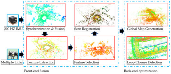
Figure 1.
Overview of multi-lidar based mapping and odometry system.
2.2. Automatic Calibration of the System
The extrinsic features of a multi lidar system need to be carefully configured before an experiment. This is generally done by detecting coincident feature points and solving the relative pose between different lidars by utilizing a target-based calibration method [29,30]. As this approach requires coincident FoVs among lidars, this is not applicable for non-overlapping systems, and thus a map-based online calibration method is often used [31,32,33,34]. As shown in Figure 2a, although the five lidars on the UGV platform do have overlapped areas, we still adopt the automatic calibration method for fast deployment.
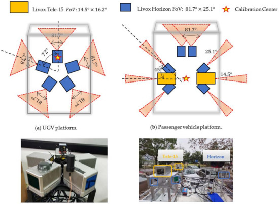
Figure 2.
The sensor configuration of our two multiple-lidar systems. The extrinsic is refined to the front-view lidar in (a), and the geometric center in (b), respectively. Five Livox Horizon lidars were included in the UGV platform, composing a FoV. While, the passenger vehicle platform had two Livox Tele-15 and six Livox Horizon lidars, with no overlaps between any two lidars.
Given two lidar coordinates, and , the goal of calibration is to determine the tranlation and rotational relation between them, denoted as and . With the assumption of an isomorphic constraint model for the environment, these two matrices can be iteratively solved using continuously constructed submaps. The Fast-lio [16] is applied for creating a precise local map, and the generalized-ICP [35] is used for map alignment. We obtain the first and from a coarse manual physical measurement, and they act as the initial guess for estimation of the exact calibration matrix. As the generalized-ICP becomes unstable and encounters mismatching errors, where obvious geometrical features are insufficient, both the calibration processes were carried out in an underground parking garage. With large registration outliers removed by random sample consensus (RANSAC) [36], the final calibration matrices could be determined after a one-minute slow driving around the garage. As can be seen in Figure 3, the geometrical structures were maintained well with the computed calibration matrix, and the best calibration accuracy was at millimeter-level after several trials.
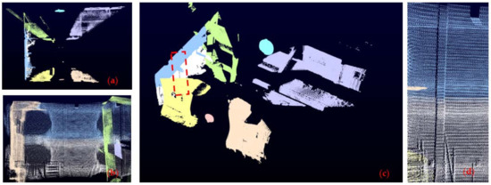
Figure 3.
Visual illustration of the calibration result for the passenger vehicle platform, with eight colors representing the respective point clouds. (a) is from the top view, while (b) is from the back view, and (c) is a 3D overview with the zoom in of a pillar shown in (d). It can be noticed that the upper half and lower half of the pillar match well with each other.
2.3. Feature Extraction
As shown in Figure 4, two different types of Livox series lidars are applied, the Livox Tele-15 and Livox Horizon. The first one is a long-range, high-density lidar, with structured circular scan pattern, the FoV is 14.5° × 16.2°. While the Horizon is totally different from Tele-15 with six laser scan diodes ‘brushing’ arbitrarily in the 81.7° × 25.1° FoV. Various lidars can be connected, either with a Livox Hub or a switch, and we used the time synchronizer in robot operation system (ROS) [37] to fuse and synchronize the lidars.
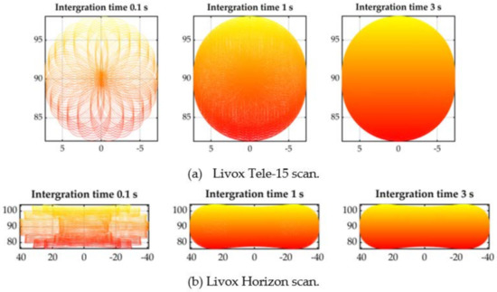
Figure 4.
Visual illustration of the two different patterns.
With the aim of allowing an arbitrary number and type of lidars to qualify for our system, we designed a parallel feature extraction process with computational efficiency. Each incoming raw lidar frame is sent to a respective thread for feature extraction, according to its ID, and the extraction methods differ between Tele-15 and Horizon.
- Tele-15:The feature points can be extracted through counting the local smoothness. Moreover, in view of the limited feature points in the tiny FoV, point reflectivity is also employed as an extra determinant. If the reflectivity of a point is different from the neighboring one for a threshold, it is also treated as an edge point.where S contains the points in the recent district, and and represent the specific coordinates of points.
- Horizon:We deployed a purely time domain feature extraction method for Horizon. All the raw point cloud data in a single frame are divided into patches with a 6 × 7 point, and an eigendecomposition is performed for the covariance of the 3D coordinates. All the 42 points are extracted as surface features if the second largest eigenvalue is 0.4 times larger than the smallest one. Then the points with the largest curvature on each scan line are found for non-surface patches, and an eigendecomposition is performed. If the largest eigenvalue is 0.3 times larger than the second largest one, the six points are extracted as edge features. Although highly accurate for feature extraction, this method can only solve low speed occasions due to the limited patch size. Therefore, a time-domain-based method is selected for the UGV platform, while a traditional approach is adopted for the passenger vehicle platform.
2.4. Feature Selection
Multiple-lidar fusion maximizes the awareness of surroundings, but inevitably extends the computation time, and data association is highly time-consuming if all the features are exploited. Furthermore, the numerous measurements from side lidars are prone to degeneration, such as the walls with planar environment and feature-poor areas in Figure 5. It would be better if only the informative features are selected and sent for optimization.
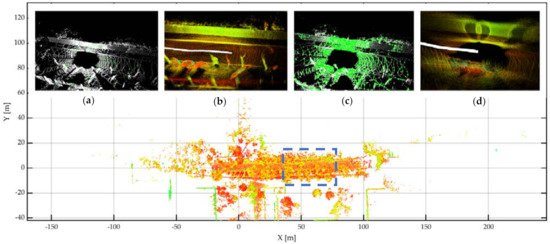
Figure 5.
A qualitative example of the good feature selection method. The UGV runs into a narrow district, where the surroundings are blocked by walls. With the lazier–greedy algorithm, only the surface features providing strong geometric constraints are picked in (a), and the local map is well maintained in (b). On the other hand, once all the surface features are imported in (c), the local map in (d) is blurred due to textureless regions. The amount of surface points in (a,c) are 1125 and 11,243, respectively.
According to [38], well-conditioned constraints should distribute in different directions, constraining the pose from different angles. For instance, parallel constraints are more susceptible to degeneracy than their orthogonal counterparts. We therefore adopted a feature selection algorithm following [39]. Features that are most valuable for estimation are selected as good features, and both the data association and state optimization should utilize only them. Denoting as the number of extracted features in one sweep, as the amount of good features set, and as the maximum number of selected features, the feature selection problem can be expressed as:
where is the information matrix of the good feature set and represents the log determinant. As a NP-hard problem, low-latency data association is guaranteed through lazier–greedy algorithm [40]. The idea is simple: at each round, the current best feature is identified only from evaluation of a random subset, while all the candidate set is searched for the simple greedy approach. With a predefined decay factor , the size of a random subset can be expressed as:
In this way, the time complexity is reduced from to , where is the constant rejection ratio. As reported in [41], the approximation ratio of a greedy approach was proven to be , thus the lazier greedy reaches a approximation guarantee in expectation of the optimal solution.
Let be the non-negative monotone and submodular function, and set the size of the random set as . Differently from the adaptive adjustment of with online degeneracy evaluation in [42], we set a constant ratio of all features for time efficiency. Let be the optimal set and the result of the lazier–greedy algorithm; achieves the approximation guarantee in expectation:
The detailed process of feature selection is summarized as follows:
- Down sample the current fused point cloud with voxel filter [43] and extract all the feature points . Set as empty at the beginning of each frame.
- For each lidar input, obtain a random subset containing elements from . For each feature point in , search the correspondence and compute the information matrix from residuals calculated from (6) and (7). Add any to that leads to maximum enhancement of the objective, . Then the is updated and replaced with .
- For each lidar input, stop step 2 until good features are found.
- Send all the good feature sets to scan registration after every thread finishes step 3.
2.5. Scan Registration
The extracted edge and surface features from different lidars are synchronized and treated as a whole. Point-to-edge and point-to-plane metrics are calculated with respect to lidar IDs and optimized together.
The scan registration starts with projecting the current point cloud into the global map , with the predefined rotational and translational relationship :
Suppose that denotes the set of all edge features in the time k + 1, for each edge feature in , the five nearest edge points in the are found, with their mean value . To make sure that they indeed form a line, the covariance matrix is computed and an eigendecomposition is performed based upon it. If the biggest eigenvalue is four times larger than the second biggest one, the five points are on a line where should lie. The point-to-edge metric is defined as follows:
here is a point among the five points, and similarly to the point-to-edge residual calculation, the five nearest surface points are searched for each surface feature in . The eigendecompositions of the covariance matrix are also computed; if the smallest eigenvalue is four-times less than the second smallest one, the five points form a plane, and the point-to-plane distance can be calculated by:
where and are the two points in the five points. The two residuals are also introduced as a measurement for dynamic object filtering. Residuals computed from (6) and (7) are sorted with one quarter of the largest residuals being removed. The pose estimation is finally performed after this process.
In the back-end, keyframes are established for global optimization, and we introduce two criteria for keyframe selection. The first is the time variation, a new keyframe is selected when the current time difference to the last keyframe exceeds 5 s, and the second is the odometry displacement, where a new keyframe is added if the distance to the last keyframe surpasses 10 m.
2.6. Scan Context Integrated Global Optimization
Place recognition provides candidates for loop closure optimization, which is critical for correcting long-term accumulating drift over a path. This is a challenging task on point cloud, as loss of textures and colors means only the geometric information is available. The well-known histogram-based methods only provide a stochastic descriptor of the scene [12], making it less discernible for place recognition problems. Thus, we follow a novel place descriptor scan context [28,44], targeting 3D lidar scan data.
With the idea of encoding the geometrical shape of the point cloud into an image, the scan context first divides a laser scan into azimuthal and radial bins in the lidar coordinate. As shown in Figure 6a, and are the number of sectors and rings. Suppose that the maximum detection range of a lidar is , then the central angle of a sector in the polar coordinate is and the radial distance between two rings is . Therefore, for each point , we have (8) describing the set of points belonging to each bin .
where , and a scan context can be encoded by assigning the maximum height of the 3D points within each bin through:
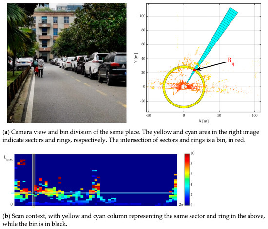
Figure 6.
Visual illustration of a challenging example of scan context.
is set as 130 m (detection range of Livox Horizon at 20% reflectivity), and . As seen in Figure 6b, the scan context partitions whole points into equally distributed intervals. Thanks to the regular encoding pattern, far points and nearby dynamic objects can be treated as sparse noise and discarded for estimation.
As can be seen in Figure 7, the place re-identification can then be simplified as column-wise similarity matching. Given a scan context pair and , the geometric similarity function can be defined as:
where and are the object and candidate column vectors at the same index. Since the column vectors describe changes in the azimuthal direction, they may be shifted even in the same place for a change of view-point. On the other hand, the row vector is dependent on the sensor location, and always consistent for the identical location. In this respect, the performance of scan context is limited in indoor environments, where variations in the vertical direction are insignificant. The change of view-point can be determined by column shifts:
where is shifted by column. The pair and can be filtered out by an empirically defined threshold, describes the best alignment of them, and is the optimal distance.
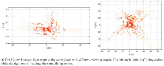

Figure 7.
Illustration of place recognition for scan context.
As a scan context is calculated for each keyframe, the candidate query will increase rapidly as vehicle moves around, and we set up a KD-tree for the fast-search of possible candidates. A local place re-identification score is defined by incorporating temporal frames into the verification:
where and are the query scan and candidate scan. This temporal score may further serve as an initial value for scan-to-scan ICP refinement.
3. Results
The performance of our approach was validated by extensive experiments on different platforms. All the datasets were processed by an onboard computer, DJI Manifold 2C, with i7-8550U, 8 GB RAM, with no GPU-accelerated computing. The proposed system can reach real-time performance with up to three lidars, and 90% and 70% real-time efficiencies are satisfied for five and eight lidars, respectively. GNSS outputs were set as ground truth for further comparison throughout all the experiments. Lever-arms were measured with a tape and stored in the hardware settings for online estimation. Results were also compared with the state-of-the-art (SOTA) following [45], with detailed description as follows.
3.1. Passenger Car Downtown Experiments
3.1.1. System Setup and Scenario Overview
Presented in Figure 2b and Figure 8, the platform consists of six Livox Horizon lidars, two Livox Tele-15 lidars, and a Livox Hub in charge of lidar connection. All the lidars are synchronized through gps-pps signals with a u-blox M8T the GNRMC format. With radio technical commissions for maritime services (RTCM) corrections from a Qianxun D100, the MTi-680G can provide RTK localizations.
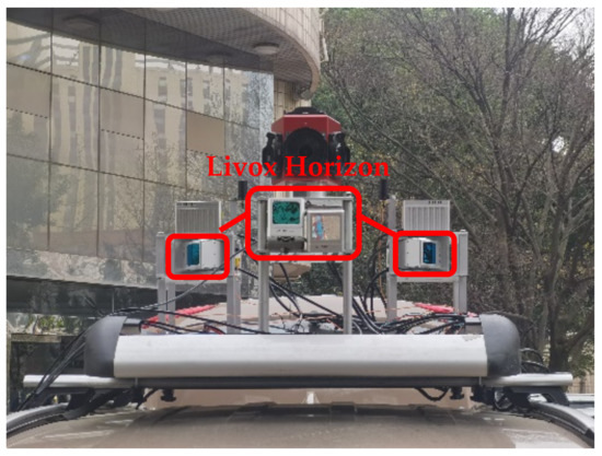
Figure 8.
Passenger car platform overview.
The up–down placement of the two front-view Livox Horizon lidars has a significant advantage in the suburbs. When heavy traffic congestion is encountered, only the upper one is introduced for mapping and map-based re-localization, ensuring accurate mapping and odometry results in highly dynamic environments.
As shown in Figure 9, two experiments were carried out on this platform: the first one was in a low-speed, low-kinematic urban scene, with the overall length and time cost of 1.5 km and 342 s. The second one tried to assess the mapping consistency in tunnels, and a long acoustic barrier on the overpass was chosen. The path is around 2 km long, with a time consumption of 141.5 s.

Figure 9.
Map illustration of the two experiments, with the red line denoting GNSS trajectory.
3.1.2. Results of Experiment #1
As the GNSS signals were occasionally blocked along the path, we only evaluated the horizontal accuracy of the proposed system with Livox Horizon Loam (official release), Lili-om, and Fast-lio. All the eight lidars were fused in our system, while only a front lidar was used for the other three methods. The following can be observed from Figure 10.
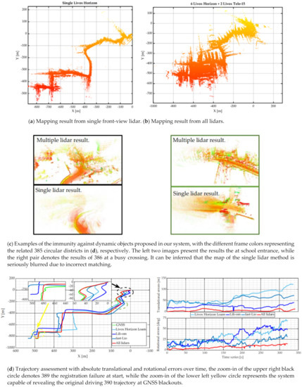
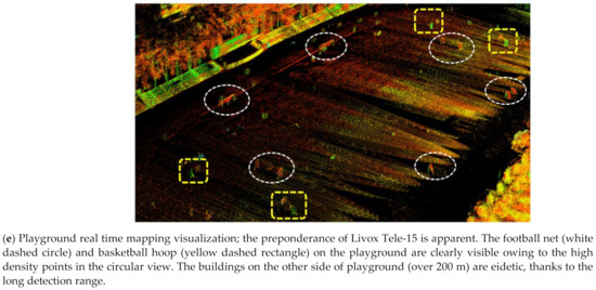
Figure 10.
Evaluation of mapping and odometry results for experiment #1.
- The advantage of integrating point clouds from multiple lidars is manifest; much more environmental information can be obtained and presented. While the front lidar mapping merely depicts the road shape, multi-lidar fusion generates generous supplementary geometrical features. Thanks to the long-range Tele-15 lidar, the playground is completely preserved on the map shown in Figure 10e. As feature quality has a great impact on lidar odometry, multi-lidar fusion should be a better approach for degeneracy problems.
- The multi-lidar fusion system was more robust than the single lidar system in dynamic scenes. The system encountered heavy congestion at the beginning, with vehicles, bicycles, and people moving irregularly. Hence the scan-to-scan correlation was difficult to determine in a severely limited FoV. We can see from Figure 10c and the upper right corner of Figure 10d that the scan registration died with front lidar only, which was the reason for the loss of other three trajectories. This is an increasingly common situation in the suburbs; with limited observable features, single lidar mapping is vulnerable to dynamic scenes. From our experience, it could be easily misled by a truck or a bus passing by, especially at crossroads, while waiting for traffic lights. With the auxiliary features from side lidars and feature filtering for front lidars, our method had the highest accuracy in these scenarios. It can be noticed from Figure 10c that the incorrect matching of dynamic objects at the beginning ruins the entire odometry. For other three single-lidar-based approaches, the initial translational error had already surpassed 10 m. While for our system, the position errors always stayed at a low level along the trajectory.
For quantitative analysis, the absolute position and orientation errors are plotted in Figure 10d for detailed reference, showing that multi-lidar fusion had a great impact on improving the positioning accuracy. The mean and the root mean square error (RMSE) of position error were 2.452 m and 3.618 m. In addition, the mean and RMSE of attitude error were 11.967° and 5.675°.
3.1.3. Results of Experiment #2
Tunnels are a great challenge to lidar odometry due to their repetitive features; with the help of an initial guess from IMU and additional feature points from side lidars, our approach was able to generate a map of tunnels with a medium length. We choose the noise barrier fence on the overhead viaducts for quantitative analysis. The selected acoustic barrier wall was blank on the top, allowing GNSS signal penetration. The laser beam was unable to go through the surrounding walls, making it share a similar pattern with traditional tunnels. The mapping and odometry result are presented in Figure 11. The RMSEs of position (3D) and attitude (RPY) error were 6.520 m and 14.567°.
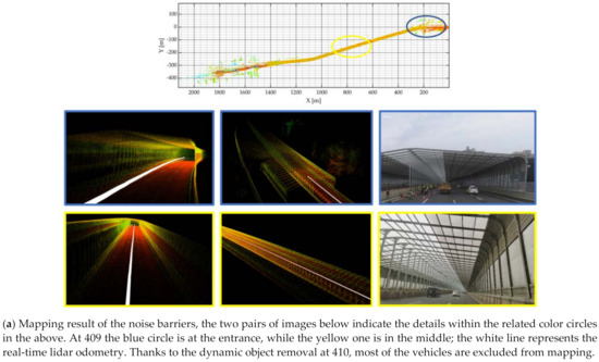
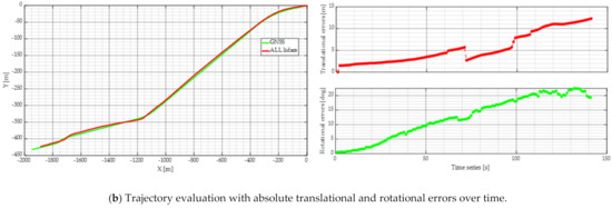
Figure 11.
Mapping and odometry results of experiment #2.
3.2. Small Platform Campus Experiments
3.2.1. System Setup and Scenario Overview
The small platform is shown in Figure 2a and Figure 12a, comprised of five Livox Horizon lidars, a MTi-680G integrated navigation unit, and a Livox Hub for lidar connection. The small platform ran at up to 5 m/s in the campus, and we used a laptop to collect all the data for fast implementation.
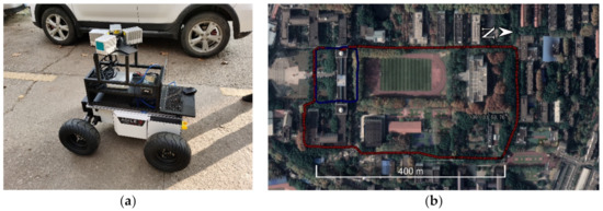
Figure 12.
Small platform setup: (a) platform overview; (b) illustration of the two loops. (blue and red trajectories).
Two loops in Wuhan university were performed to validate our approach, shown in Figure 12b, the first one is a small loop around the main building, with a time consumption of 283 s and overall length 600 m, while the second one is a big loop, 852 s in all, and around 1.8 km. As there are trees and buildings blocking the GNSS signals along the path, we only evaluated the horizontal position and roll-pitch attitude accuracy in this case.
3.2.2. Effects of Lidar Number
Since our scheme supports an arbitrary number of lidars for optimization, we first investigate the performance variation with respect to lidar number. The small loop is selected for illustration here, and Figure 13 describes the results from various numbers of lidars. With each of them carrying out pure odometry, no global optimization was enabled. As a result, the following was discovered.
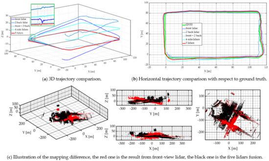
Figure 13.
Illustration of multi-lidar fusion improvements.
- A five-lidar fusion could eliminate the exaggerated height ramp of a single lidar approach. There were six speed bumpers on the path, causing large vertical vibrations to the vehicle. Some of these perpendicular motions are fatal to lidar odometry, as vertical displacement will be enlarged by incorrect registrations. The front lidar trajectory in Figure 13a encountered a vertical dump in the left corner, which was the result of two consecutive speed bump. With limited FoV from only the front view, the single lidar odometry was unable to correct these errors; it was further affected by error propagation in Figure 13c. Extending extra constraint features from side lidars, our approach was able to correct these errors and maintain a flat terrain.
- The geometry of multiple lidar placement made a significant improvement to the system performance. We can notice from Figure 13a that the results from one front view lidar and two back view lidars had the most proximal accuracy with the five-lidar fusion. On the other hand, the positioning error of two back lidars was worse than the single front view lidar. Therefore, pentagon-like and triangle-like multi-lidar setups should deliver better mapping and positioning results in real cases.
3.2.3. Effects of Loop Closure Optimization
As shown in Figure 14, the big loop was taken into consideration here, and two other place representations were selected for comparison: a pose-information-based loop detector [46] and a histogram-based loop detector. The pose-information-based loop detection encountered the most exaggerated errors, in the top left corner. With the assumption of small pose deviations along the path, the pose-information-based approach took keyframes of similar poses as a detected loop. Therefore, this method is unable to handle large-scale mapping, where pose deviation is inevitable. Histogram-based loop detection also failed to close the loop, and the part in the green circle distorted seriously. As a feature-based method, it is hard to avoid the influence of dynamic objects and view angle variations with this approach. Since only a scan context was encapsulated for each scan, this descriptor had the best accuracy for challenging scenes, with the 2D translational and roll-pitch rotational RMSEs of 1.997 m and 7.198°.
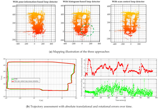
Figure 14.
Description of the effects on loop closure optimization.
3.2.4. Comparison with Mechanical Lidar
Each Livox Horizon lidar has a horizontal view of 81.7°, with five of them completing a full coverage of 360°, which is similar to traditional mechanical lidars. Here, two widely known lidars, Ouster OS1-64 and Velodyne VLP-16, were chosen for evaluation with our multi-lidar method. We selected three popular algorithms for demonstration, a tightly coupled Lio-sam [47], an advanced implementation of LOAM (A-LOAM), and LeGO-LOAM. Both the Lio-sam and LeGO-LOAM were also integrated with scan context as a global descriptor. The experiments on two loops are illustrated here, with the mapping results presented in Figure 15, and the following information can be observed.
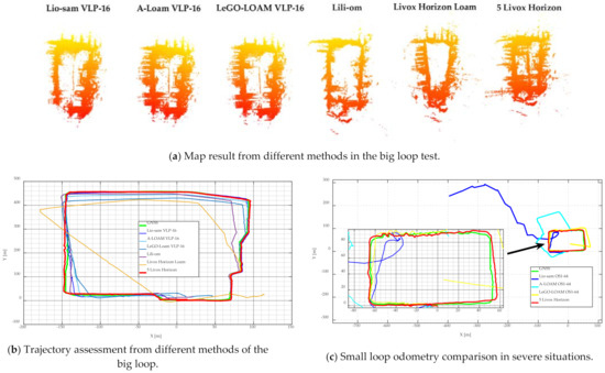
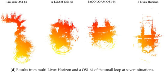
Figure 15.
Mapping and odometry evaluation of 5 Livox Horizons and mechanical lidar.
- Multi-lidar fusion had a commendable mapping accuracy and retained abundant features in the meantime. In the current market, the five Livox Horizon kit is (5 Livox Horizons and a Livox Hub) almost the same price as a VLP-16, and half the cost of an OS1-64. Moreover, the horizontal odometry results in Figure 15b and Table 1 also indicate that our approach had an accuracy comparable with Lio-sam.
 Table 1. Horizontal position error statistics of the big loop. (Compared with Velodyne VLP-16).
 - Multi-lidar fusion had a better performance in challenging scenarios. Shown in Figure 15c,d we carried out an experiment of small loop at class breaktime, with students and vehicles blocking the paths. Therefore, our vehicle had to avoid collisions with irregular motions, such as moving back and forth, sharp turnings, and fast accelerations. Lio-sam had the most significant failure in such areas, because of loss of landmark constraints. Since the IMU pre-integration process of the system depends heavily on lidar odometry [48], the system was liable to fail once the landmark constraint information was insufficient. The maximum error of A-LOAM came from back-and-forth motions, causing a more than 90° deviation to the trajectory. The starting area was a crowded pathway with vehicles on both sides; as our platform was much lower than common sedans, most of the surface points were cast on vehicles. Once the front view is blocked by pedestrians, the loops cannot be detected or are mismatched, hence LeGO-LOAM failed to close the loop. A crucial benefit of multi-lidar fusion is the capability of manipulating each lidar input freely. With a pre-set empirical threshold for the amount of edge points, all the edge and surface features from the individual lidars after selection were further down sampled to 10% of their original size once the threshold was reached. This is similar to shutting down some typical view angles of a mechanical lidar, and thus alleviating bad impacts in certain areas. Moreover, the major part of dynamic objects in the front view can be removed by point-to-edge and point-to-plane residuals. With the help of the two mentioned improvements, our multi-lidar fusion solution had a strong capability in severe situations, and the end-to-end errors were small, as presented in Table 2.
 Table 2. End-to-end position and attitude errors for the small loop at severe situations. (Compared with Ouster OS1-64).
4. Conclusions
In this work, we proposed a robust mapping and odometry algorithm for multiple non-repetitive scanning lidars. The robustness is ensured mainly through two approaches, the first is good feature selection against massive data and degeneracy, and the latter is the novel place descriptor against dynamic objects and view angle variations. Extensive experiments on two platforms were conducted. The results show that the proposed algorithm delivers superior accuracy over SOTA single lidar methods.
There are several directions for future research. Adding additional GNSS measurements into our system is conceivable, which would further compensate for accumulated drifts and maintain the global map. Another research direction concerns map reuse. With a great variety of lidars on the market, challenges still remain for map-based re localization. It would be desirable if we could use low-cost lidars or even cameras to register high-definition maps.
Author Contributions
Conceptualization, Y.W.; methodology, Y.W., Y.Z. and F.H.; software, Y.W. and F.H.; validation, Y.W., W.S., Z.T. and F.H.; formal analysis, Y.W. and F.H.; investigation, W.S. and Z.T.; resources, Y.W., W.S. and Z.T.; data curation, Y.W.; writing—original draft preparation, Y.W.; writing—review and editing, Y.L. and Y.Z.; visualization, Y.W.; supervision, Y.L.; project administration, W.S.; funding acquisition, W.S. and Y.L. All authors have read and agreed to the published version of the manuscript.
Funding
This research was funded by National Key Research and Development Project of China, grant number 2017YFB0503401-01, and the Joint Foundation for Ministry of Education of China, grant number 6141A02011907.
Institutional Review Board Statement
Not applicable.
Informed Consent Statement
Not applicable.
Data Availability Statement
The experiment #1 data is available at: https://drive.google.com/file/d/1xCSo3WEE2eeHfw2nxp-tJhLZzecE9No8/view?usp=sharing, accessed on 17 April 2021; Please notice only the two front-view Horizon, two side-view Tele-15, IMU, GNSS data is included here due to limited Google Drive storage space. The small loop data including 5 Livox Horizon, IMU and GNSS is available at: https://drive.google.com/file/d/1foRGNXSi0Bk699Ye1u9vDfVas0eM8Cer/view?usp=sharing, accessed on 17 April 2021; For those who are interested, please contact Yusheng Wang for more data and algorithms.
Conflicts of Interest
The authors declare no conflict of interest.
References
- Liu, R.; Wang, J.; Zhang, B. High definition map for automated driving: Overview and analysis. J. Navig. 2020, 73, 324–341. [Google Scholar] [CrossRef]
- Bresson, G.; Alsayed, Z.; Yu, L.; Glaser, S. Simultaneous localization and mapping: A survey of current trends in autonomous driving. IEEE Trans. Intell. Veh. 2017, 2, 194–220. [Google Scholar] [CrossRef]
- Campos, C.; Elvira, R.; Rodríguez, J.J.G.; Montiel, J.M.; Tardós, J.D. ORB-SLAM3: An accurate open-source library for visual, visual-inertial and multi-map SLAM. arXiv 2020, arXiv:2007.11898. [Google Scholar]
- Qin, T.; Li, P.; Shen, S. Vins-mono: A robust and versatile monocular visual-inertial state estimator. IEEE Trans. Robot. 2018, 34, 1004–1020. [Google Scholar] [CrossRef]
- Cvišić, I.; Ćesić, J.; Marković, I.; Petrović, I. SOFT-SLAM: Computationally efficient stereo visual simultaneous localization and mapping for autonomous unmanned aerial vehicles. J. Field Robot. 2018, 35, 578–595. [Google Scholar] [CrossRef]
- Bénet, P.; Guinamard, A. Robust and Accurate Deterministic Visual Odometry. In Proceedings of the 33rd International Technical Meeting of the Satellite Division of the Institute of Navigation (ION GNSS+ 2020), Virtual Program, 21–25 September 2020; pp. 2260–2271. [Google Scholar]
- Taketomi, T.; Uchiyama, H.; Ikeda, S. Visual SLAM algorithms: A survey from 2010 to 2016. IPSJ Trans. Comput. Vis. Appl. 2017, 9, 1–11. [Google Scholar] [CrossRef]
- Zhang, J.; Singh, S. LOAM: Lidar Odometry and Mapping in Real-time. In Proceedings of the Robotics: Science and Systems, Berkeley, CA, USA, 12–16 July 2014; Volume 2. [Google Scholar]
- Liu, Z.; Zhang, F.; Hong, X. Low-cost retina-like robotic lidars based on incommensurable scanning. IEEE ASME Trans. Mechatron. 2021. [Google Scholar] [CrossRef]
- Glennie, C.L.; Hartzell, P.J. Accuracy Assessment and Calibration of Low-Cost Autonomous LIDAR Sensors. Int. Arch. Photogramm. Remote Sens. Spat. Inf. Sci. 2020, 43, 371–376. [Google Scholar] [CrossRef]
- Lin, J.; Zhang, F. Loam livox: A fast, robust, high-precision LiDAR odometry and mapping package for LiDARs of small FoV. In Proceedings of the 2020 IEEE International Conference on Robotics and Automation (ICRA), Paris, France, 31 May–31 August 2020; pp. 3126–3131. [Google Scholar]
- Lin, J.; Zhang, F. A fast, complete, point cloud based loop closure for lidar odometry and mapping. arXiv 2019, arXiv:1909.11811. [Google Scholar]
- Livox and Xpeng Partner to Bring Mass Produced, Built-In Lidar to the Market. Available online: https://www.livoxtech.com/news/14 (accessed on 7 April 2021).
- Joint Collaboration between Livox, Zhito and FAW Jiefang Propels Autonomous Heavy-Duty Truck into the Smart Driving Era. Available online: https://www.livoxtech.com/news/11 (accessed on 7 April 2021).
- Li, K.; Li, M.; Hanebeck, U.D. Towards high-performance solid-state-lidar-inertial odometry and mapping. IEEE Robot. Autom. Lett. 2021. [Google Scholar] [CrossRef]
- Xu, W.; Zhang, F. Fast-lio: A fast, robust lidar-inertial odometry package by tightly-coupled iterated kalman filter. IEEE Robot. Autom. Lett. 2021, 6, 3317–3332. [Google Scholar] [CrossRef]
- Sun, P.; Kretzschmar, H.; Dotiwalla, X.; Chouard, A.; Patnaik, V.; Tsui, P.; Guo, J.; Zhou, Y.; Chai, Y.; Caine, B. Scalability in perception for autonomous driving: Waymo open dataset. In Proceedings of the IEEE/CVF Conference on Computer Vision and Pattern Recognition, Seattle, WA, USA, 14–19 June 2020; pp. 2446–2454. [Google Scholar]
- Liu, T.; Liao, Q.; Gan, L.; Ma, F.; Cheng, J.; Xie, X.; Wang, Z.; Chen, Y.; Zhu, Y.; Zhang, S. Hercules: An autonomous logistic vehicle for contact-less goods transportation during the covid-19 outbreak. arXiv 2020, arXiv:2004.07480. [Google Scholar]
- Geyer, J.; Kassahun, Y.; Mahmudi, M.; Ricou, X.; Durgesh, R.; Chung, A.S.; Hauswald, L.; Pham, V.H.; Mühlegg, M.; Dorn, S. A2d2: Audi autonomous driving dataset. arXiv 2020, arXiv:2004.06320. [Google Scholar]
- Jiao, J.; Yun, P.; Tai, L.; Liu, M. MLOD: Awareness of Extrinsic Perturbation in Multi-LiDAR 3D Object Detection for Autonomous Driving. arXiv 2020, arXiv:2010.11702. [Google Scholar]
- Lin, J.; Liu, X.; Zhang, F. A decentralized framework for simultaneous calibration, localization and mapping with multiple LiDARs. arXiv 2020, arXiv:2007.01483. [Google Scholar]
- Jiao, J.; Ye, H.; Zhu, Y.; Liu, M. Robust Odometry and Mapping for Multi-LiDAR Systems with Online Extrinsic Calibration. arXiv 2020, arXiv:2010.14294. [Google Scholar]
- Fenwick, J.W.; Newman, P.M.; Leonard, J.J. Cooperative concurrent mapping and localization. In Proceedings of the 2002 IEEE International Conference on Robotics and Automation (Cat. No. 02CH37292), Washington, DC, USA, 11–15 May 2002; Volume 2, pp. 1810–1817. [Google Scholar]
- Tao, T.; Huang, Y.; Yuan, J.; Sun, F.; Wu, X. Cooperative simultaneous localization and mapping for multi-robot: Approach & experimental validation. In Proceedings of the 2010 8th World Congress on Intelligent Control and Automation, Jinan, China, 6–9 July 2010; pp. 2888–2893. [Google Scholar]
- Nettleton, E.; Thrun, S.; Durrant-Whyte, H.; Sukkarieh, S. Decentralised SLAM with low-bandwidth communication for teams of vehicles. In Proceedings of the Field and Service Robotics; Springer: Berlin/Heidelberg, Germany, 2003; pp. 179–188. [Google Scholar]
- Nettleton, E.; Durrant-Whyte, H.; Sukkarieh, S. A robust architecture for decentralised data fusion. In Proceedings of the Proceedings of the International Conference on Advanced Robotics (ICAR), Coimbra, Portugal, 30 June 30–3 July 2003. [Google Scholar]
- Durrant-Whyte, H. A Beginner’s Guide to Decentralised Data Fusion; Technical Document of Australian Centre for Field Robotics; University of Sydney: Sydney, Australia, 2000; pp. 1–27. [Google Scholar]
- Kim, G.; Kim, A. Scan context: Egocentric spatial descriptor for place recognition within 3d point cloud map. In Proceedings of the 2018 IEEE/RSJ International Conference on Intelligent Robots and Systems (IROS), Madrid, Spain, 1–5 October 2018; pp. 4802–4809. [Google Scholar]
- Cui, J.; Niu, J.; Ouyang, Z.; He, Y.; Liu, D. ACSC: Automatic Calibration for Non-repetitive Scanning Solid-State LiDAR and Camera Systems. arXiv 2020, arXiv:2011.08516. [Google Scholar]
- Zhang, Z. A flexible new technique for camera calibration. IEEE Trans. Pattern Anal. Mach. Intell. 2000, 22, 1330–1334. [Google Scholar] [CrossRef]
- Jiao, J.; Yu, Y.; Liao, Q.; Ye, H.; Fan, R.; Liu, M. Automatic calibration of multiple 3d lidars in urban environments. In Proceedings of the 2019 IEEE/RSJ International Conference on Intelligent Robots and Systems (IROS), Macau, China, 3–8 November 2019; pp. 15–20. [Google Scholar]
- Lv, J.; Xu, J.; Hu, K.; Liu, Y.; Zuo, X. Targetless Calibration of LiDAR-IMU System Based on Continuous-time Batch Estimation. arXiv 2020, arXiv:2007.14759. [Google Scholar]
- Eckenhoff, K.; Geneva, P.; Bloecker, J.; Huang, G. Multi-camera visual-inertial navigation with online intrinsic and extrinsic calibration. In Proceedings of the 2019 International Conference on Robotics and Automation (ICRA), Montreal, QC, Canada, 20–24 May 2019; pp. 3158–3164. [Google Scholar]
- Lepetit, V.; Moreno-Noguer, F.; Fua, P. Epnp: An accurate o (n) solution to the pnp problem. Int. J. Comput. Vis. 2009, 81, 155. [Google Scholar] [CrossRef]
- Segal, A.; Haehnel, D.; Thrun, S. Generalized-icp. In Proceedings of the Robotics: Science and systems, Seattle, WA, USA, 28 June–1 July 2009; Volume 2, p. 435. [Google Scholar]
- Fischler, M.A.; Bolles, R.C. Random sample consensus: A paradigm for model fitting with applications to image analysis and automated cartography. Commun. Acm 1981, 24, 381–395. [Google Scholar] [CrossRef]
- Quigley, M.; Conley, K.; Gerkey, B.; Faust, J.; Foote, T.; Leibs, J.; Wheeler, R.; Ng, A.Y. ROS: An open-source Robot Operating System. In Proceedings of the ICRA workshop on open source software, Kobe, Japan, 12–17 May 2009; Volume 3, p. 5. [Google Scholar]
- Zhang, J.; Kaess, M.; Singh, S. On degeneracy of optimization-based state estimation problems. In Proceedings of the 2016 IEEE International Conference on Robotics and Automation (ICRA), Stockholm, Sweden, 16–21 May 2016; pp. 809–816. [Google Scholar]
- Zhao, Y.; Vela, P.A. Good Feature Matching: Toward Accurate, Robust VO/VSLAM with Low Latency. IEEE Trans. Robot. 2020, 36, 657–675. [Google Scholar] [CrossRef]
- Mirzasoleiman, B.; Badanidiyuru, A.; Karbasi, A.; Vondrák, J.; Krause, A. Lazier than lazy greedy. In Proceedings of the Proceedings of the AAAI Conference on Artificial Intelligence, Austin, TX, USA, 25–29 January 2015; Voulme 29. [Google Scholar]
- Summers, T.H.; Cortesi, F.L.; Lygeros, J. On submodularity and controllability in complex dynamical networks. IEEE Trans. Control Netw. Syst. 2015, 3, 91–101. [Google Scholar] [CrossRef]
- Jiao, J.; Zhu, Y.; Ye, H.; Huang, H.; Yun, P.; Jiang, L.; Wang, L.; Liu, M. Greedy-Based Feature Selection for Efficient LiDAR SLAM. arXiv 2021, arXiv:2103.13090. [Google Scholar]
- Rusu, R.B.; Cousins, S. 3d is here: Point cloud library (pcl). In Proceedings of the 2011 IEEE International Conference on Robotics and Automation, Shanghai, China, 9–13 May 2011; pp. 1–4. [Google Scholar]
- Wang, H.; Wang, C.; Xie, L. Intensity scan context: Coding intensity and geometry relations for loop closure detection. In Proceedings of the 2020 IEEE International Conference on Robotics and Automation (ICRA), Paris, France, 31 May–31 August 2020; pp. 2095–2101. [Google Scholar]
- Zhang, Z.; Scaramuzza, D. A tutorial on quantitative trajectory evaluation for visual (-inertial) odometry. In Proceedings of the 2018 IEEE/RSJ International Conference on Intelligent Robots and Systems (IROS), Madrid, Spain, 1–5 October 2018; pp. 7244–7251. [Google Scholar]
- Shan, T.; Englot, B. Lego-loam: Lightweight and ground-optimized lidar odometry and mapping on variable terrain. In Proceedings of the 2018 IEEE/RSJ International Conference on Intelligent Robots and Systems (IROS), Madrid, Spain, 1–5 October 2018; pp. 4758–4765. [Google Scholar]
- Shan, T.; Englot, B.; Meyers, D.; Wang, W.; Ratti, C.; Rus, D. Lio-sam: Tightly-coupled lidar inertial odometry via smoothing and mapping. arXiv 2020, arXiv:2007.00258. [Google Scholar]
- Kaess, M.; Johannsson, H.; Roberts, R.; Ila, V.; Leonard, J.J.; Dellaert, F. iSAM2: Incremental smoothing and mapping using the Bayes tree. Int. J. Robot. Res. 2012, 31, 216–235. [Google Scholar] [CrossRef]
Publisher’s Note: MDPI stays neutral with regard to jurisdictional claims in published maps and institutional affiliations. |
© 2021 by the authors. Licensee MDPI, Basel, Switzerland. This article is an open access article distributed under the terms and conditions of the Creative Commons Attribution (CC BY) license (https://creativecommons.org/licenses/by/4.0/).