
Spatial Analyses and Susceptibility Modeling of Thermokarst Lakes in Permafrost Landscapes along the Qinghai–Tibet Engineering Corridor

 ,
,
Abstract

1. Introduction
2. Study Area
3. Methods and Data
3.1. Satellite Data and Processing
3.2. Spatial Analyses
3.3. Machine Learning-Based Susceptibility Analysis
3.3.1. Machine Learning Model
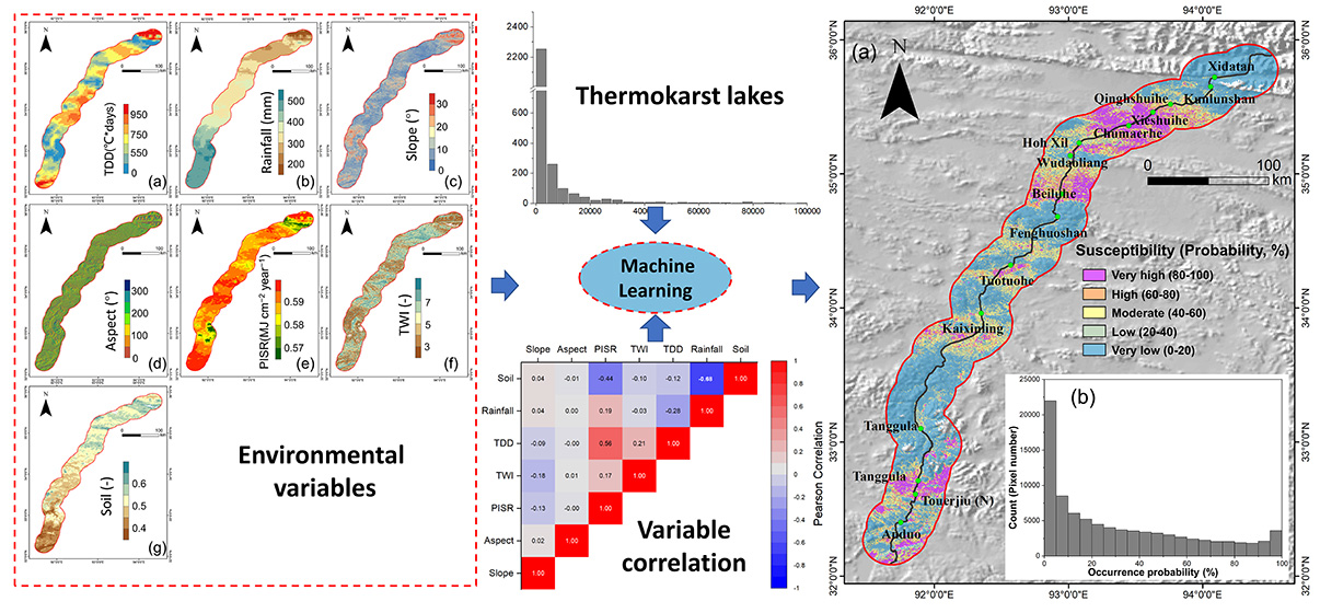
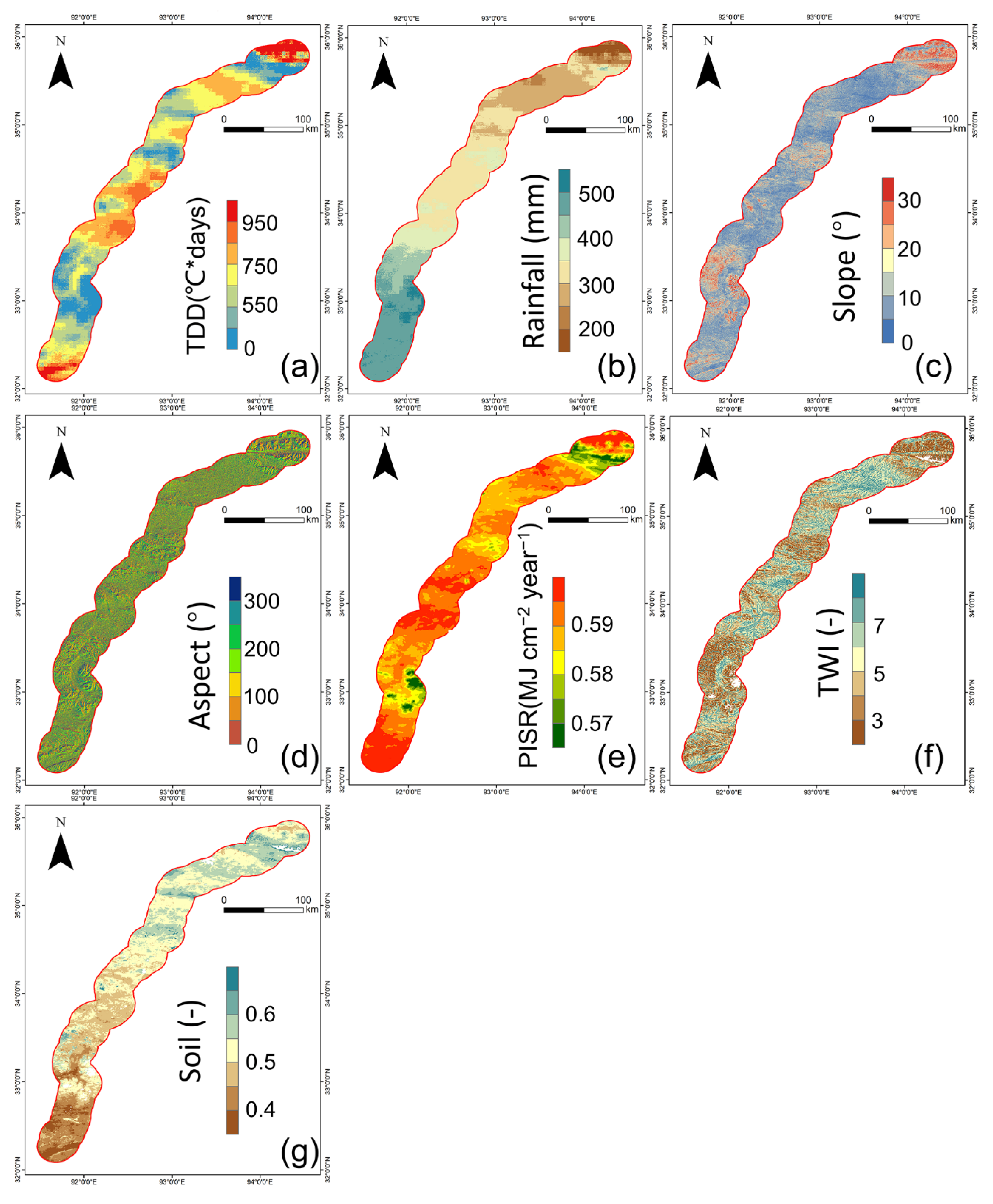
3.3.2. Environmental Variables
3.3.3. Model Performance
3.4. Producing TLS Maps
3.5. Other Statistical Analysis
4. Results
4.1. Spatial Distribution of TLs
4.2. Model Performance
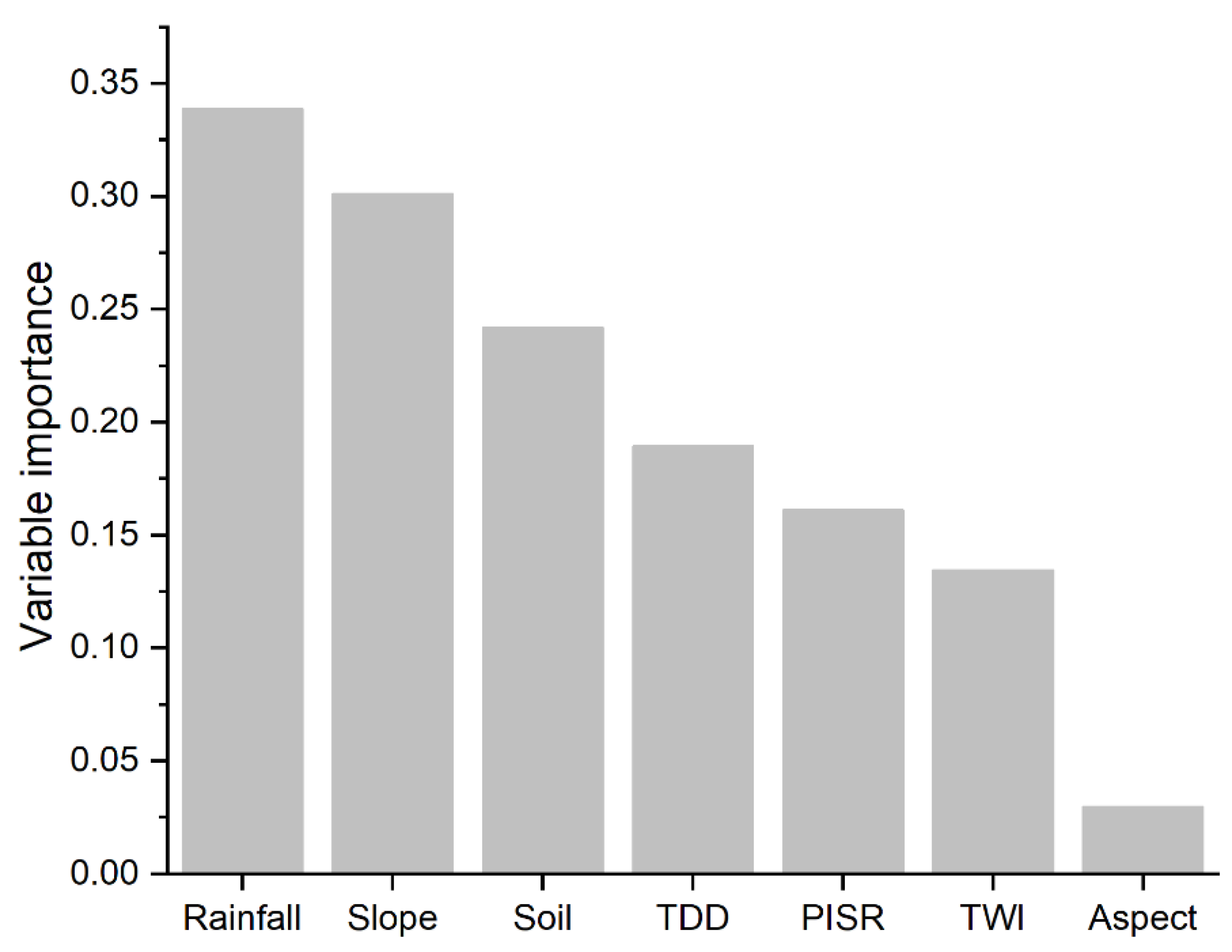
4.3. Environmental Variable Importance
4.4. Thermokarst Lake Susceptibility Map
5. Discussion
5.1. Spatial Distribution and Development of TLs
5.2. Environmental Control Factors
5.3. Implications of the TLS Modeling
6. Conclusions
Supplementary Materials
Author Contributions
Funding
Data Availability Statement
Acknowledgments
Conflicts of Interest
References
- Obu, J.; Westermann, S.; Bartsch, A.; Berdnikov, N.; Christiansen, H.H.; Dashtseren, A.; Delaloye, R.; Elberling, B.; Etzelmüller, B.; Kholodov, A.; et al. Northern Hemisphere permafrost map based on TTOP modelling for 2000–2016 at 1 km2 scale. Earth-Sci. Rev. 2019, 193, 299–316. [Google Scholar] [CrossRef]
- Biskaborn, B.K.; Smith, S.L.; Noetzli, J.; Matthes, H.; Vieira, G.; Streletskiy, D.A.; Schoeneich, P.; Romanovsky, V.E.; Lewkowicz, A.G.; Abramov, A.; et al. Permafrost is warming at a global scale. Nat. Commun. 2019, 10, 264. [Google Scholar] [CrossRef] [PubMed]
- Aalto, J.; Karjalainen, O.; Hjort, J.; Luoto, M. Statistical forecasting of current and future circum-Arctic ground temperatures and active layer thickness. Geophys. Res. Lett. 2018, 45, 4889–4898. [Google Scholar] [CrossRef]
- Guo, D.; Wang, H. CMIP5 permafrost degradation projection: A comparison among different regions. J. Geophys. Res. Atmos. 2016, 121, 4499–4517. [Google Scholar] [CrossRef]
- Osterkamp, T.E.; Jorgenson, M.T.; Schuur, E.A.G.; Shur, Y.L.; Kanevskiy, M.Z.; Vogel, J.G.; Tumskoy, V.E. Physical and ecological changes associated with warming permafrost and thermokarst in Interior Alaska. Permafr. Periglac. Process. 2009, 20, 235–256. [Google Scholar] [CrossRef]
- Nitzbon, J.; Westermann, S.; Langer, M.; Martin, L.C.P.; Strauss, J.; Laboor, S.; Boike, J. Fast response of cold ice-rich permafrost in northeast Siberia to a warming climate. Nat. Commun. 2020, 11, 2201. [Google Scholar] [CrossRef]
- Grosse, G.; Harden, J.; Turetsky, M.; McGuire, A.D.; Camill, P.; Tarnocai, C.; Frolking, S.; Schuur, E.A.G.; Jorgenson, T.; Marchenko, S.; et al. Vulnerability of high-latitude soil organic carbon in North America to disturbance. J. Geophys. Res. Space Phys. 2011, 116. [Google Scholar] [CrossRef]
- Qiu, J. The third pole. Nature 2008, 454, 24. [Google Scholar] [CrossRef]
- Zou, D.; Zhao, L.; Sheng, Y.; Chen, J.; Hu, G.; Wu, T.; Wu, J.; Xie, C.; Wu, X.; Pang, Q.; et al. A new map of permafrost distribution on the Tibetan Plateau. Cryosphere 2017, 11, 2527–2542. [Google Scholar] [CrossRef]
- Yang, M.; Wang, X.; Pang, G.; Wan, G.; Liu, Z. The Tibetan Plateau cryosphere: Observations and model simulations for current status and recent changes. Earth-Sci. Rev. 2019, 190, 353–369. [Google Scholar] [CrossRef]
- Zhao, L.; Wu, Q.; Marchenko, S.; Sharkhuu, N. Thermal state of permafrost and active layer in Central Asia during the international polar year. Permafr. Periglac. Process. 2010, 21, 198–207. [Google Scholar] [CrossRef]
- Li, R.; Wu, Q.; Li, X.; Sheng, Y.; Hu, G.; Cheng, G.; Zhao, L.; Jin, H.; Zou, D.; Wu, X. Characteristic, changes and impacts of permafrost on Qinghai-Tibet Plateau. Chin. Sci. Bull. 2019, 64, 2783–2795. [Google Scholar] [CrossRef]
- Wu, Q.; Zhang, T.; Liu, Y. Thermal state of the active layer and permafrost along the Qinghai-Xizang (Tibet) Railway from 2006 to 2010. Cryosphere 2012, 6, 607–612. [Google Scholar] [CrossRef]
- Wu, Q.; Zhang, Z.; Gao, S.; Ma, W. Thermal impacts of engineering activities and vegetation layer on permafrost in different alpine ecosystems of the Qinghai–Tibet Plateau, China. Cryosphere 2016, 10, 1695–1706. [Google Scholar] [CrossRef]
- Grosse, G.; Goetz, S.; McGuire, A.D.; Romanovsky, V.E.; Schuur, E.A.G. Changing permafrost in a warming world and feedbacks to the Earth system. Environ. Res. Lett. 2016, 11, 040201. [Google Scholar] [CrossRef]
- Kokelj, S.V.; Jorgenson, M.T. Advances in Thermokarst Research. Permafr. Periglac. Process. 2013, 24, 108–119. [Google Scholar] [CrossRef]
- Olefeldt, D.; Goswami, S.; Grosse, G.; Hayes, D.; Hugelius, G.; Kuhry, P.; McGuire, A.D.; Romanovsky, V.E.; Sannel, A.; Schuur, E.; et al. Circumpolar distribution and carbon storage of thermokarst landscapes. Nat. Commun. 2016, 7, 13043. [Google Scholar] [CrossRef] [PubMed]
- Walter, K.M.; Zimov, S.A.; Chanton, J.P.; Verbyla, D.; Chapin, F.S. Methane bubbling from Siberian thaw lakes as a positive feedback to climate warming. Nat. Cell Biol. 2006, 443, 71–75. [Google Scholar] [CrossRef]
- Luo, J.; Niu, F.; Lin, Z.; Liu, M.; Yin, G. Thermokarst lake changes between 1969 and 2010 in the Beilu River Basin, Qinghai–Tibet Plateau, China. Sci. Bull. 2015, 60, 556–564. [Google Scholar] [CrossRef]
- Niu, F.; Luo, J.; Lin, Z.; Liu, M.; Yin, G. Morphological Characteristics of Thermokarst Lakes along the Qinghai-Tibet Engineering Corridor. Arct. Antarct. Alp. Res. 2014, 46, 963–974. [Google Scholar] [CrossRef]
- Grosse, G.; Jones, B.; Arp, C. Thermokarst Lakes, Drainage, and Drained Basins. In Treatise on Geomorphology; Shroder, J.F., Ed.; Academic Press: San Diego, CA, USA, 2013; pp. 325–353. [Google Scholar]
- Lin, Z.; Luo, J.; Niu, F. Development of a thermokarst lake and its thermal effects on permafrost over nearly 10 yr in the Beiluhe Basin, Qinghai-Tibet Plateau. Geosphere 2016, 12, 632–643. [Google Scholar] [CrossRef]
- Lin, Z.; Niu, F.; Xu, Z.; Xu, J.; Wang, P. Thermal regime of a thermokarst lake and its influence on permafrost, Beiluhe Basin, Qinghai-Tibet Plateau. Permafr. Periglac. Process. 2010, 21, 315–324. [Google Scholar] [CrossRef]
- Niu, F.; Lin, Z.; Liu, H.; Lu, J. Characteristics of thermokarst lakes and their influence on permafrost in Qinghai–Tibet Plateau. Geomorphology 2011, 132, 222–233. [Google Scholar] [CrossRef]
- Lin, Z.; Niu, F.; Fang, J.; Luo, J.; Yin, G. Interannual variations in the hydrothermal regime around a thermokarst lake in Beiluhe, Qinghai-Tibet Plateau. Geomorphology 2017, 276, 16–26. [Google Scholar] [CrossRef]
- Ling, F.; Wu, Q.; Zhang, T.; Niu, F. Modelling Open-Talik Formation and Permafrost Lateral Thaw under a Thermokarst Lake, Beiluhe Basin, Qinghai-Tibet Plateau. Permafr. Periglac. Process. 2012, 23, 312–321. [Google Scholar] [CrossRef]
- Jin, H.; Wei, Z.; Wang, S.; Yu, Q.; Lü, L.; Wu, Q.; Ji, Y. Assessment of frozen-ground conditions for engineering geology along the Qinghai–Tibet highway and railway, China. Eng. Geol. 2008, 101, 96–109. [Google Scholar] [CrossRef]
- Zhao, L.; Zou, D.; Hu, G.; Du, E.; Pang, Q.; Xiao, Y.; Li, R.; Sheng, Y.; Wu, X.; Sun, Z.; et al. Changing climate and the permafrost environment on the Qinghai–Tibet (Xizang) plateau. Permafr. Periglac. Process. 2020, 31, 396–405. [Google Scholar] [CrossRef]
- Zhou, T.; Zhang, W. Anthropogenic warming of Tibetan Plateau and constrained future projection. Environ. Res. Lett. 2021, 16, 044039. [Google Scholar] [CrossRef]
- Wu, Q.; Zhang, T. Changes in active layer thickness over the Qinghai-Tibetan Plateau from 1995 to 2007. J. Geophys. Res. Space Phys. 2010, 115. [Google Scholar] [CrossRef]
- Chen, H.; Zhu, Q.; Peng, C.; Wu, N.; Wang, Y.; Fang, X.; Gao, Y.; Zhu, D.; Yang, G.; Tian, J.; et al. The Impacts of Climate Change and Human Activities on Biogeochemical Cycles on the Qinghai-Tibetan Plateau. Glob. Chang. Biol. 2013, 19, 2940–2955. [Google Scholar] [CrossRef]
- Niu, F.; Yin, G.; Luo, J.; Lin, Z.; Liu, M. Permafrost Distribution along the Qinghai-Tibet Engineering Corridor, China Using High-Resolution Statistical Mapping and Modeling Integrated with Remote Sensing and GIS. Remote Sens. 2018, 10, 215. [Google Scholar] [CrossRef]
- Gao, Z.; Lin, Z.; Niu, F.; Luo, J.; Liu, M.; Yin, G. Hydrochemistry and controlling mechanism of lakes in permafrost regions along the Qinghai-Tibet Engineering Corridor, China. Geomorphology 2017, 297, 159–169. [Google Scholar] [CrossRef]
- Morgenstern, A.; Grosse, G.; Günther, F.; Fedorova, I.; Schirrmeister, L. Spatial analyses of thermokarst lakes and basins in Yedoma landscapes of the Lena Delta. Cryosphere 2011, 5, 849–867. [Google Scholar] [CrossRef]
- ESRI. ArcGIS Desktop: Release 10.2.2; Environmental Systems Research Institute: Redlands, CA, USA, 2014. [Google Scholar]
- Zhao, L.; Zou, D.; Hu, G.; Wu, T.; Du, E.; Liu, G.; Xiao, Y.; Li, R.; Pang, Q.; Qiao, Y.; et al. A synthesis dataset of permafrost thermal state for the Qinghai-Xizang (Tibet) Plateau, China. Earth Syst. Sci. Data Discuss. 2021, 2021, 1–22. [Google Scholar]
- Breiman, L. Random forests. Mach. Learn. 2001, 45, 5–32. [Google Scholar] [CrossRef]
- Belgiu, M.; Drăguţ, L. Random forest in remote sensing: A review of applications and future directions. ISPRS J. Photogramm. Remote Sens. 2016, 114, 24–31. [Google Scholar] [CrossRef]
- Karjalainen, O.; Luoto, P.M.; Aalto, J.; Etzelmuller, P.B.; Grosse, G.; Jones, B.M.; Lilleøren, K.S.; Hjort, J. High potential for loss of permafrost landforms in a changing climate. Environ. Res. Lett. 2020, 15, 104065. [Google Scholar] [CrossRef]
- Aalto, J.; Luoto, M. Integrating climate and local factors for geomorphological distribution models. Earth Surf. Process. Landf. 2014, 39, 1729–1740. [Google Scholar] [CrossRef]
- Marmion, M.; Hjort, J.; Thuiller, W.; Luoto, M. A comparison of predictive methods in modelling the distribution of periglacial landforms in Finnish Lapland. Earth Surf. Process. Landf. 2008, 33, 2241–2254. [Google Scholar] [CrossRef]
- R Core Team. R: A Language and Environment for Statistical Computing; R Foundation for Statistical Computing: Vienna, Austria, 2020; Available online: http://www.R-project.org/ (accessed on 1 March 2021).
- Thuiller, W.; Georges, D.; Engler, R.; Breiner, F. Biomod2: Ensemble Platform for Species Distribution Modeling. R Package Version: 3.4.6. Available online: https://cran.r-project.org/web/packages/biomod2/ (accessed on 1 March 2021).
- Thuiller, W.; Lafourcade, B.; Engler, R.; Araújo, M.B. BIOMOD—A platform for ensemble forecasting of species distributions. Ecography 2009, 32, 369–373. [Google Scholar] [CrossRef]
- Karjalainen, O.; Luoto, M.; Aalto, J.; Hjort, J. New insights into the environmental factors controlling the ground thermal regime across the Northern Hemisphere: A comparison between permafrost and non-permafrost areas. Cryosphere 2019, 13, 693–707. [Google Scholar] [CrossRef]
- Frauenfeld, O.W.; Zhang, T.; McCreight, J.L. Northern Hemisphere freezing/thawing index variations over the twentieth century. Int. J. Clim. 2006, 27, 47–63. [Google Scholar] [CrossRef]
- Yang, K.; He, J. China Meteorological Forcing Dataset (1979–2018); National Tibetan Plateau Data Center: Beijing, China, 2019. [Google Scholar]
- Fiddes, J.; Gruber, S. TopoSCALE v.1.0: Downscaling gridded climate data in complex terrain. Geosci. Model Dev. 2014, 7, 387–405. [Google Scholar] [CrossRef]
- Zhang, H.; Zhang, F.; Zhang, G.; Che, T.; Yan, W. How Accurately Can the Air Temperature Lapse Rate over the Tibetan Plateau Be Estimated from MODIS LSTs? J. Geophys. Res. Atmos. 2018, 123, 3943–3960. [Google Scholar] [CrossRef]
- Guo, X.; Wang, L.; Tian, L. Spatio-temporal variability of vertical gradients of major meteorological observations around the Tibetan Plateau. Int. J. Clim. 2016, 36, 1901–1916. [Google Scholar] [CrossRef]
- Jarvis, A.; Reuter, H.I.; Nelson, A.; Guevara, E. Hole-filled SRTM for the Globe Version 4, Available from the CGIAR-CSI SRTM 90m Database. 2008. Available online: http://srtm.csi.cgiar.org (accessed on 1 February 2021).
- Cheng, G. The mechanism of repeated-segregation for the formation of thick layered ground ice. Cold Reg. Sci. Technol. 1983, 8, 57–66. [Google Scholar]
- Kokelj, S.V.; Burn, C.R. Near-surface ground ice in sediments of the Mackenzie Delta, Northwest Territories, Canada. Permafr. Periglac. Process. 2005, 16, 291–303. [Google Scholar] [CrossRef]
- Hengl, T.; De Jesus, J.M.; Heuvelink, G.B.M.; Gonzalez, M.R.; Kilibarda, M.; Blagotić, A.; Shangguan, W.; Wright, M.N.; Geng, X.; Bauer-Marschallinger, B.; et al. SoilGrids250m: Global gridded soil information based on machine learning. PLoS ONE 2017, 12, e0169748. [Google Scholar] [CrossRef]
- Allouche, O.; Tsoar, A.; Kadmon, R. Assessing the accuracy of species distribution models: Prevalence, kappa and the true skill statistic (TSS). J. Appl. Ecol. 2006, 43, 1223–1232. [Google Scholar] [CrossRef]
- Zhang, G.; Yao, T.; Piao, S.; Bolch, T.; Xie, H.; Chen, D.; Gao, Y.; O’Reilly, C.M.; Shum, C.K.; Yang, K.; et al. Extensive and drastically different alpine lake changes on Asia’s high plateaus during the past four decades. Geophys. Res. Lett. 2017, 44, 252–260. [Google Scholar] [CrossRef]
- Zhang, G.; Yao, T.; Shum, C.K.; Yi, S.; Yang, K.; Xie, H.; Feng, W.; Bolch, T.; Wang, L.; Behrangi, A.; et al. Lake volume and groundwater storage variations in Tibetan Plateau’s endorheic basin. Geophys. Res. Lett. 2017, 44, 5550–5560. [Google Scholar] [CrossRef]
- Farquharson, L.; Mann, D.; Grosse, G.; Jones, B.; Romanovsky, V. Spatial distribution of thermokarst terrain in Arctic Alaska. Geomorphology 2016, 273, 116–133. [Google Scholar] [CrossRef]
- Hinkel, K.M.; Frohn, R.C.; Nelson, F.E.; Eisner, W.R.; Beck, R.A. Morphometric and spatial analysis of thaw lakes and drained thaw lake basins in the western Arctic Coastal Plain, Alaska. Permafr. Periglac. Process. 2005, 16, 327–341. [Google Scholar] [CrossRef]
- Côté, M.M.; Burn, C.R. The oriented lakes of Tuktoyaktuk Peninsula, Western Arctic Coast, Canada: A GIS-based analysis. Permafr. Periglac. Process. 2002, 13, 61–70. [Google Scholar] [CrossRef]
- Grosse, G.; Romanovsky, V.; Walter, K.; Morgenstern, A.; Lantuit, H.; Zimov, S. Distribution of Thermokarst Lakes and Ponds at Three Yedoma Sites in Siberia in International Conference on Permafrost; Institute of Northern Engineering, University of Alaska Fairbanks: Fairbanks, AK, USA, 2008. [Google Scholar]
- Lin, Z.; Gao, Z.; Fan, X.; Niu, F.; Luo, J.; Yin, G.; Liu, M. Factors controlling near surface ground-ice characteristics in a region of warm permafrost, Beiluhe Basin, Qinghai-Tibet Plateau. Geoderma 2020, 376, 114540. [Google Scholar] [CrossRef]
- French, H.M. The Periglacial Environment; John Wiley and Sons: Hoboken, NJ, USA, 2007. [Google Scholar]
- French, H.; Shur, Y. The principles of cryostratigraphy. Earth-Sci. Rev. 2010, 101, 190–206. [Google Scholar] [CrossRef]
- Gao, Z.; Niu, F.; Wang, Y.; Lin, Z.; Wang, W. Suprapermafrost groundwater flow and exchange around a thermokarst lake on the Qinghai–Tibet Plateau, China. J. Hydrol. 2021, 593, 125882. [Google Scholar] [CrossRef]
- Mu, C.; Abbott, B.W.; Norris, A.J.; Mu, M.; Fan, C.; Chen, X.; Jia, L.; Yang, R.; Zhang, T.; Wang, K.; et al. The status and stability of permafrost carbon on the Tibetan Plateau. Earth-Sci. Rev. 2020, 211, 103433. [Google Scholar] [CrossRef]
- Walvoord, M.A.; Kurylyk, B.L. Hydrologic Impacts of Thawing Permafrost—A Review. Vadose Zone J. 2016, 15, 1–20. [Google Scholar] [CrossRef]


| Section | MAAT (°C)/Rainfall (mm) | Landform | Vegetation | Surficial Geology | MAGT (°C) | Ground Ice Condition | Lake Number |
|---|---|---|---|---|---|---|---|
| Qinghusihe–Chumaerhe (QC) | −4.1/527 | Upland alluvial plain | Alpine meadow | Silt loam and clay | −1.0~−0.7 | Ice rich (>50%) and ice saturated | 11,423 |
| Wudaoliang–Beiluhe (WB) | −4.5/312 | Upland denudation platform and basin | Alpine meadow and Sparse grassland | Silt loam and clay | −2.0~−2.4 | Ice-saturated and ice layers with soils | 4074 |
| TuoTuohe (TTH) | −3.5/302 | Upland pluvial plain | Alpine steppe | Silt loam | −0.1~0.1 | Less ice and talik | 1520 |
| Kaixinling (KXL) | −3.2/370 | Upland alluvial plain | Alpine meadow | Loamy sand | −0.8~−0.7 | Ice-saturated and ice layers with soils | 1533 |
| Tanggula (TGL) | −4.7/352 | Upland till plain | Alpine meadow | Loamy sand | −0. 8~−1.2 | Ice rich (>50%) | 5392 |
| Anduo (AD) | −2.2/459 | Upland alluvial and pluvial plain | Alpine meadow | Silty clay | 0~−0.1 | Ice rich (>50%) | 4746 |
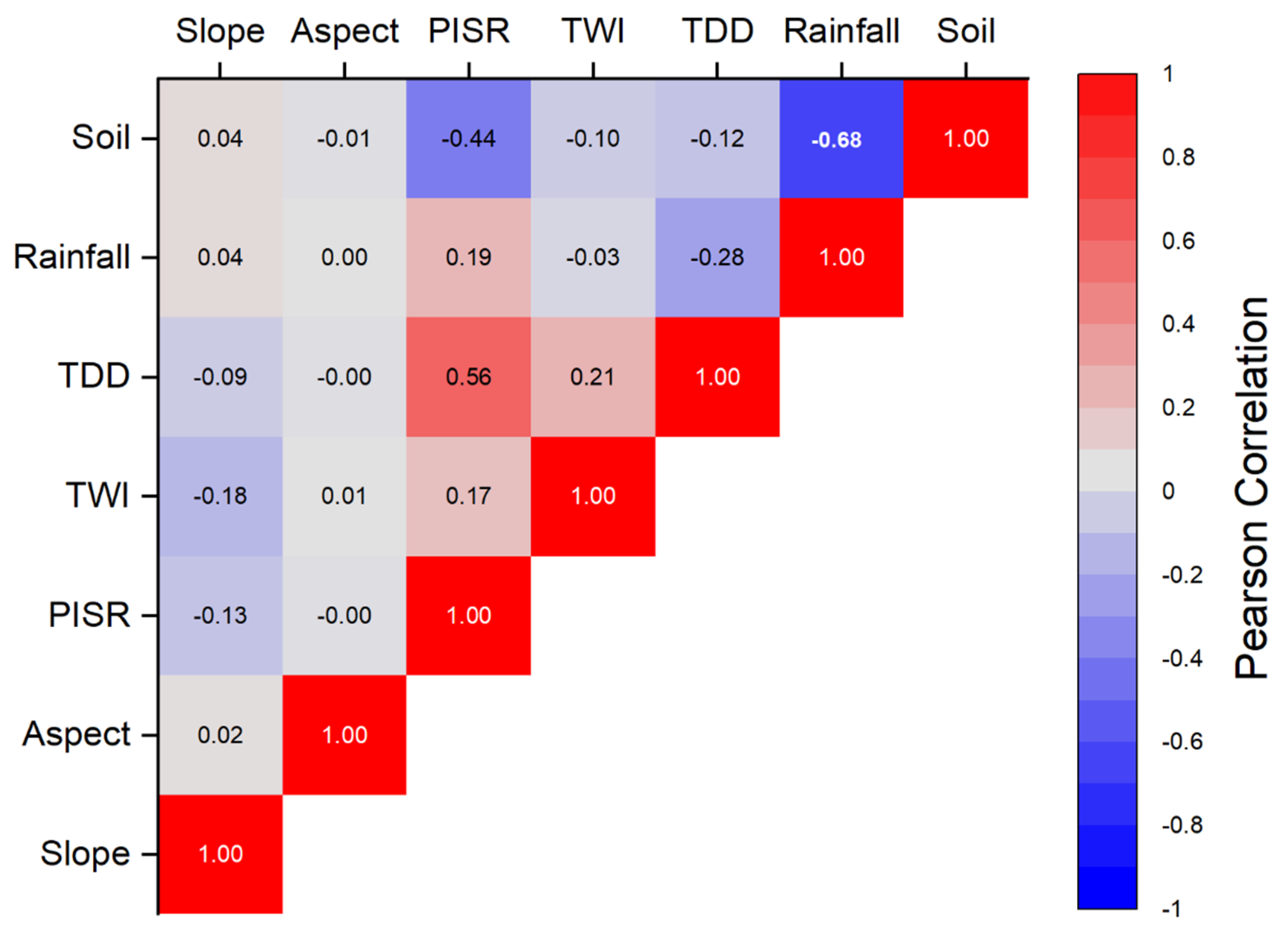
| Variable | Slope | Aspect | PISR | TWI | TDD | Rainfall | Soil |
|---|---|---|---|---|---|---|---|
| VIF | 1.05 | 1.00 | 1.86 | 1.08 | 2.30 | 4.80 | 4.58 |
Publisher’s Note: MDPI stays neutral with regard to jurisdictional claims in published maps and institutional affiliations. |
© 2021 by the authors. Licensee MDPI, Basel, Switzerland. This article is an open access article distributed under the terms and conditions of the Creative Commons Attribution (CC BY) license (https://creativecommons.org/licenses/by/4.0/).
Share and Cite
Yin, G.; Luo, J.; Niu, F.; Zhou, F.; Meng, X.; Lin, Z.; Liu, M. Spatial Analyses and Susceptibility Modeling of Thermokarst Lakes in Permafrost Landscapes along the Qinghai–Tibet Engineering Corridor. Remote Sens. 2021, 13, 1974. https://doi.org/10.3390/rs13101974
Yin G, Luo J, Niu F, Zhou F, Meng X, Lin Z, Liu M. Spatial Analyses and Susceptibility Modeling of Thermokarst Lakes in Permafrost Landscapes along the Qinghai–Tibet Engineering Corridor. Remote Sensing. 2021; 13(10):1974. https://doi.org/10.3390/rs13101974
Chicago/Turabian StyleYin, Guoan, Jing Luo, Fujun Niu, Fujun Zhou, Xianglian Meng, Zhanju Lin, and Minghao Liu. 2021. "Spatial Analyses and Susceptibility Modeling of Thermokarst Lakes in Permafrost Landscapes along the Qinghai–Tibet Engineering Corridor" Remote Sensing 13, no. 10: 1974. https://doi.org/10.3390/rs13101974
APA StyleYin, G., Luo, J., Niu, F., Zhou, F., Meng, X., Lin, Z., & Liu, M. (2021). Spatial Analyses and Susceptibility Modeling of Thermokarst Lakes in Permafrost Landscapes along the Qinghai–Tibet Engineering Corridor. Remote Sensing, 13(10), 1974. https://doi.org/10.3390/rs13101974