Abstract
Plant phenology depends largely on temperature, but temperature alone cannot explain the Northern Hemisphere shifts in the start of the growing season (SOS). The spatio–temporal distribution of SOS sensitivity to climate variability has also changed in recent years. We applied the partial least squares regression (PLSR) method to construct a standardized SOS sensitivity evaluation index and analyzed the combined effects of air temperature (Tem), water balance (Wbi), radiation (Srad), and previous year’s phenology on SOS. The spatial and temporal distributions of SOS sensitivity to Northern Hemisphere climate change from 1982 to 2014 were analyzed using time windows of 33 and 15 years; the dominant biological and environmental drivers were also assessed. The results showed that the combined sensitivity of SOS to climate change (SCom) is most influenced by preseason temperature sensitivity. However, because of the asymmetric response of SOS to daytime/night temperature (Tmax/Tmin) and non-negligible moderating of Wbi and Srad on SOS, SCom was more effective in expressing the effect of climate change on SOS than any single climatic factor. Vegetation cover (or type) was the dominant factor influencing the spatial pattern of SOS sensitivity, followed by spring temperature (Tmin > Tmax), and the weakest was water balance. Forests had the highest SCom absolute values. A significant decrease in the sensitivity of some vegetation (22.2%) led to a decreasing trend in sensitivity in the Northern Hemisphere. Although temperature remains the main climatic factor driving temporal changes in SCom, the temperature effects were asymmetric between spring and winter (Tems/Temw). More moisture might mitigate the asymmetric response of SCom to spring/winter warming. Vegetation adaptation has a greater influence on the temporal variability of SOS sensitivity relative to each climatic factor (Tems, Temw, Wbi, Srad). More moisture might mitigate the asymmetric response of SCom to spring/winter warming. This study provides a basis for vegetation phenology sensitivity assessment and prediction.
1. Introduction
Plant phenology, especially the start of the growing season (SOS) (or spring green-up date), is a highly sensitive indicator of the impacts of climate change on the biosphere [1,2,3]. The early onset of vegetation spring phenology has been widely reported as an indicator of the climate warming [1,3,4]. Vegetation phenology fine-tunes itself according to the environment; moreover, it is closely linked to climate variability [5,6]. Studies have shown that earlier SOS leads to higher photosynthetic rates and vegetation growth [7], while also increasing transpiration, resulting in increased drought stress [8]. Phenological changes also regulate vegetation feedback to the climate system by influencing the regional and global carbon budget, water flux, and energy balance [4,9]. Therefore, improving the knowledge on phenology change and its drivers is essential to better understand and model the relationship between ecosystems and the climate system.
Plant phenological sensitivity (phenological phase changes caused by unit changes in climatic conditions) determines the magnitude of phenological changes in response to future climate change and is key to understanding the relationship between vegetation phenology and climate change [3,10]. A number of studies have extensively assessed the impacts of global warming on the SOS over the past decades based on ground and satellite data [10,11,12,13,14,15,16,17,18,19,20,21]. Temperature is considered the dominant controlling factor of SOS [13,14,17,18], and studies on phenological sensitivity have also focused on the sensitivity of SOS to temperature (STem) [22,23,24]. However, the relative importance of climate constraints on surface phenology has shifted since 1982 [13]. Recent studies have found that precipitation may play a key role in determining the spring [10,12]. Moreover, snow cover produced by preseason precipitation has also been shown to influence spring phenology at high latitudes and altitudes [15]. Radiation, a comprehensive measure of sunshine duration and light intensity, shows obvious interannual variability [16]. Moreover, the photoperiod plays an important role in controlling SOS in most Northern Hemisphere forests [17]. Radiation indirectly affects phenology, as it influences preseason temperature and water balance by controlling surface heat fluxes and evapotranspiration. Importantly, biological factors can also modulate the SOS [10,16]. The interaction between phenological events in spring and autumn may change the overall phenological response to climate warming [10]. Although SOS is influenced by multiple meteorological factors, most studies have examined only the temperature or precipitation sensitivity of SOS [22,23,24]; only a few studies have evaluated the combined effects of climate change on SOS [25]. This is partly because preseason meteorological factors, such as temperature, moisture utilization, and radiation, have different units of measurement. As a result, the sensitivity of each meteorological factor based on regression analysis cannot be quantitatively compared on the same scale. In addition, considering the STem as an example, the length of the phenologically relevant period (preseason) affected by temperature (including Tem, Tmax, and Tmin) varies in different climatic regions (or biomes), and changes in the temperature cumulative time and statistical characteristics may cause estimation biases in STem [22,25]. SOS responds differently to Tmax and Tmin for the same preseason duration in some areas [18]; this difference in response is controlled by a number of environmental factors and vegetation conditions [10]. Thus, the phenological response of vegetation to recent climate warming cannot be explained entirely by temperature [26,27]. Given the complex response of SOS to preseason meteorological elements and biological elements, most previous studies were single factor sensitivity studies based on linear regression analysis (univariate and multiple regression) [24] and correlation analysis (or partial correlation analysis) [28]. Therefore, it is necessary to establish a standardized sensitivity evaluation index considering the influence of biological factors to characterize the sensitivity of SOS to each meteorological factor, which would facilitate a comparative analysis of the SOS sensitivity to each meteorological factor, and to construct a comprehensive SOS sensitivity index for climate change.
The spatio–temporal differences in the sensitivity of SOS to climate change are not yet fully understood. The STem exhibits a large spatial variability [26] and has a downward trend with global warming [12,29,30]. Fu et al. [29] reported a declining STem in European temperate tree species. The causes for the spatio–temporal variation of STem are poorly understood, particularly on the global scale [10,24]. Studies have explored the causes of variation in phenological sensitivity from the aspects of climate, geography, and biology [12,23,24,25,28,31,32,33,34,35]. Interacting effects of temperature and precipitation have changed the climate sensitivity of spring vegetation green-up [25]. The SOS is more sensitive to pre-season precipitation in arid areas and more sensitive to preseason temperature in humid areas [12]. With warming-induced leaf-out advancement, a reduced photoperiod earlier in spring may decrease the STem [10]. The sensitivity of spring vegetation phenology is related to the rate of warming and phenological sensitivity with increasing local spring temperature variance at the species level from ground observations [23]. Spring phenological temperature sensitivity is higher at low latitudes than at cold or high latitudes [34,35]. The sensitivity of vegetation phenology to climate change varies by biome [32]; vegetation types with earlier SOSmean (mean SOS for 1982–2008) are more sensitive to spring temperature in the Northern Hemisphere [28]. Changes in phenological sensitivity are the result of a combination of multiple factors, but few studies have analyzed the dominant drivers of sensitivity variation. Understanding the large-scale spatio–temporal pattern of phenological sensitivity to climate change and its dominant controls will improve our ability to predict the timing of SOS.
In this study, we used four different methods to extract phenology dates from the normalized difference vegetation index (NDVI) time series of the Global Inventory Monitoring and Modeling System (GIMMS) NDVI3g.v1 dataset. We then applied the partial least squares regression (PLSR) to extract the standardized SOS sensitivity index to preseason climatic factors (air temperature, water balance, and radiation) and constructed a comprehensive SOS sensitivity index (SCom) for climate change. The purpose of this study was to (1) quantify the spatial and temporal variability of the Northern Hemisphere (latitude ≥ 30°) SOS sensitivity to climate change (single factor and synthesis) from 1982 to 2014 in 33-year and 15-year time windows, (2) determine the influence of environmental and biological factors on the spatial distribution of SOS sensitivity, and (3) identify the dominant drivers of the temporal variability of SOS sensitivity.
2. Materials and Methods
2.1. Materials
The NDVI is widely used in global-scale phenological studies [10,20]. In this study, we used the latest NDVI dataset (GIMMS NDVI3g.v1 https://iridl.ldeo.columbia.edu/SOURCES/.NASA/.ARC/.ECOCAST/.GIMMS/.NDVI3g/.v1p0/ (Accessed 15 May 2021) generated from NOAA/AVHRR series satellite images by the NASA GIMMS group, which covers the period from January 1982 to December 2015 and has a spatial resolution of 1/12° and an interval of 15 days [36]. NDVI3g.v1 addresses various issues that were present in earlier datasets addressed in NDVI3g.v1 (e.g., updating satellite sensors, atmospheric disturbances, and non-vegetation dynamics), and NDVI3g.v1 further addresses the artifacts caused by snow cover and calibration changes [37]. In this study, we excluded areas of bare soil/sparse vegetation with an annual average NDVI of less than 0.1 [20].
TerraClimate is a high-resolution (1/24°, 4 km) global monthly climate and climatic water balance dataset covering the period from 1958 to 2015 [38]. It combines high spatial resolution WorldClim climate data with coarse resolution data from other sources to generate monthly precipitation, maximum and minimum temperatures, wind speed, vapor pressure, and solar radiation datasets. TerraClimate also uses a water balance model to generate monthly surface water balance datasets. Compared with coarser datasets, TerraClimate shows significant improvement with regard to spatial authenticity and the overall mean absolute error. We used the monthly average maximum temperature (Tmax), average minimum temperature (Tmin), accumulated precipitation (Pre), downward shortwave flux at the surface (Srad), soil moisture (Sm), actual evapotranspiration (Aet), and snow water equivalent (Swe) TerraClimate datasets covering 1981–2015.
The land cover (LC) data product from the European Space Agency’s Climate Change Initiative (CCI) specifies different vegetation types. The project delivers consistent global land-cover maps at a spatial resolution of 300 m and an annual temporal resolution from 1992 to 2015. The land cover classification system used in this dataset was found to be compatible with the plant functional types used in climate models [39]. We used the new and improved Köppen–Geiger climate classification maps at 1-km resolution [40] for the present day (1980–2016) to specify the different climate regions by referring to the Intergovernmental Panel on Climate Change (IPCC) default climate regions recalculated by the Joint Research Centre (JRC) of the European Commission [41]. We excluded grid points where phenology could not be extracted and land cover types changed, especially for pixels with two or more growth cycles in one year. Detailed information and spatial distribution of climatic regions and plant types are shown in Table 1 and Figure 1. The spatial resolution of the land cover and climatic regions was resampled to match the resolution of the NDVI data.

Table 1.
Descriptions of the climatic regions and plant types in this study based on the Köppen climate classification and CCI-LC land cover types, respectively.
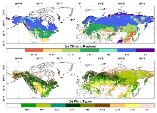
Figure 1.
Spatial distribution of climatic regions (a) and plant types (b).
2.2. Methods
2.2.1. Extracting Phenology Using NDVI Data
A number of methods have been developed to extract the SOS and EOS (end of the growing season) from seasonal NDVI variability. Phenology extraction is mainly divided into two steps: (1) reconstructing the NDVI time series, and (2) determining the phenological extraction from the change characteristics of the filtered NDVI curve. We used the double logistic function to fit the NDVI time series in this study [20]. The inflection point detection method or the threshold method can be used to extract phenological data from NDVI time series data. We used two inflection point detection methods (i.e., first-order derivative [42] and second-order derivative [43] methods) and two fixed threshold methods (i.e., 0.2 [44] and 0.5 [45] fixed thresholds), to obtain a total of four methods to extract vegetation SOS and EOS in the Northern Hemisphere from 1982 to 2014. To reduce the uncertainty caused by the different methods, we used the average SOS and EOS of the four methods. Savizky–Golay filters were applied to the GIMMS NDVI3g.v1 datasets to minimize noise prior to phenological estimation [20].
2.2.2. Partial Least Squares Regression (PLSR)
PLSR is a multivariate statistical regression analysis that combines the advantages of multiple regression, typical correlation, and principal component analysis. It is advantageous in the analysis of multiple variables with multiple correlations, particularly when the number of variables is greater than the number of samples [46]. The standardized model regression coefficient (MC), an output of PLSR, indicates the extent to which the independent variables can explain the weight of the dependent variables. In this study, MC was defined as the normalization sensitivity of the dependent variable to the independent variable. Variable importance in the projection (VIP) is an important output of PLSR and represents the relative importance of independent variables in explaining the dependent variable in the model. When VIP ≥ 1, the independent variable is considered important and that it significantly affects the dependent variable [47]. The independent variable could be considered the dominant driver of the dependent variable when its VIP value is maximum and greater than 1. PLSR is widely used in the study of vegetation response to climate change and has played an important role in identifying influential factors in both lag and driving force analyses [36,47,48]. In this study, all variables were standardized before PLSR analysis.
2.2.3. Sensitivity of SOS to Climate Change
The process for calculating the sensitivity of the SOS to climate change (Figure 2) is as follows:
- (1)
- Screening of indicators: Meteorological and biological factors can affect SOS. Therefore, we selected Tmax, Tmin, Pre, Aet, melting snow water equivalent (Ms), effective precipitation (Water = Pre − Aet), water balance index (Wbi = Pre − Aet − Ms), Sm, and Srad as meteorological variables in this study covering the six months of preseason; the lengths of the growing season (LOS), EOS, and SOS of the previous year were selected as biological variables. We performed a PLSR for each pixel using 57 (9 × 6 months + 3) indicators as independent variables and SOS as the dependent variable. Ms was calculated as the difference between the month’s snow water equivalent (Swe) and that of the previous month. Based on our PLSR results in the Northern Hemisphere and the specific physical significance, we selected Tmax, Tmin, Wbi, and Srad as the final climatic indicators and the previous year’s EOS and LOS as the final biological indicators affecting SOS in this study.
- (2)
- Optimal preseason determination: The end date of the preseason is usually fixed as the SOS date. Therefore, the start date should be optimized to strengthen the correlation between preseason climatic factors and phenology [29,33]. Based on the PLSR results, we defined preseason in this study as the period during which the preseason climatic factors (preseason average Tmax and Tmin, cumulative Wbi, and cumulative Srad at a time step of one month) showed the highest contribution to SOS dynamics in each pixel, that is, when the VIP value was at its maximum. The weather data for the month in which the SOS was located were used to calculate the preseason length when the SOS date occurred after the 15th [16]; this approach retains the influence of biological factors with a total of 26 (4 × 6 months + 2) independent variables. In this step, we obtained 20 optimal preseason datasets, each of which included the best preseason duration of Tmax, Tmin, Wbi, and Srad for each pixel in the Northern Hemisphere, one on a 33-year time window and the remaining 19 on a 15-year time window.
- (3)
- Standardized sensitivity index: To analyze the spatial distribution and temporal variability of SOS sensitivity to climatic factors in the Northern Hemisphere during 1982–2014, we conducted a PLSR for each pixel between SOS and the optimal preseason meteorological (mean Tmax, mean Tmin, cumulative Wbi, cumulative Srad) and biological (EOS and LOS of the previous year) factors with time windows of 33 and 15 years, respectively. MC is the standardized sensitivity index, and VIP is the relative importance of each climatic factor. SCom is the sum of the MC values of the four climatic factors. Finally, we obtained 20 sensitivity datasets, each of which included the sensitivity of SOS to preseason Tmax, Tmin, Tem, Wbi, Srad, and Com for each pixel in the Northern Hemisphere.

Figure 2.
Calculation process of SOS sensitivity to climate change.
Figure 2.
Calculation process of SOS sensitivity to climate change.

2.2.4. Effect Evaluation of the Sensitivity Index
A high standard deviation indicates dispersion across a wide range of values in a time series [49]. The standard deviation (SD) index, which only represents the stability of SOS under the influence of climate factors—was used with the standardized sensitivity index for the Spearman correlation analysis. Higher absolute values of the correlation coefficient indicate a stronger effect of the sensitivity index. The formula for calculating the SD index is as follows:
where is the standard deviation of the SOS time series from 1982 to 2015, indicating the stability of SOS; is the determination coefficient of PLSR, which represents the contribution of climatic and biological factors to SOS dynamics; and is the weight of the meteorological factors. The SD index can therefore be used to measure the SOS fluctuations caused by climate change, with larger SD values indicating weaker SOS resistance to climate change.
2.2.5. Trend Analysis and Significance Testing
The Mann–Kendall (MK) trend test is a commonly used method for measuring hydrological, meteorological, and other non-normally distributed time-series trends. We used the Then–Sen (TS) estimator and the non-parametric MK test for trend analysis and significance testing of the sensitivity index. The TS–MK method minimizes the noise related to parametric uncertainty in the regression equation [50]. The climate tendency rate is a method to describe the long-term meteorological trends; the linear tendency method was used to calculate the climate tendency rate of each climatic factor for each pixel, where p < 0.05 indicates a significant change. The sensitivity intensity in this study was expressed as the absolute value of the sensitivity for trend analysis and driving force analysis.
2.2.6. Driving Force Analysis
The PLSR method was used to determine the influence of spring (March to May) climate (Tmin, Tmax, Wbi, Srad), spring climate tendency rate (Tmin’, Tmax’, Wbi’, Srad’), biological (mean value of NDVI and SOS), and geographical (altitude and latitude) factors on the spatial distribution of SCom in the Northern Hemisphere during 1982–2014 with time windows of 33 and 15 years. The PLSR method was also used to explore the relative importance of climatic (average temperature in spring, average temperature in winter—December to February, accumulated Wbi in spring and winter—December to May, accumulated Srad in spring and winter) and biological (mean value of SOS with a 15-year time window) factors driving the temporal variation of SCom in each pixel. The values of MC and VIP obtained by the PLSR represent the respective driving direction and relative importance of each driving factor that affected the spatio–temporal variation of sensitivity.
3. Results
3.1. Selection of Indicators and Preseason Duration for Sensitivity Assessment
Reasonable light, temperature, and moisture indicators can help us obtain more accurate SOS sensitivity to climate change. Statistical results on the influence of meteorological variables covering the six months of the preseason and previous year’s phenology on SOS in the Northern Hemisphere (Figure 3a) showed that meteorological variables had the strongest influence on SOS during the month in which SOS occurred, and the intensity of the impact then decreased with increasing months. Tmax had the strongest impact on SOS followed by Tmin. The correlation between SOS and Tmax and Tmin may be the opposite (Figure 3b). Among the water-related indicators, Aet had the strongest effect on SOS followed by Ms. This may be due to the direct effect of temperature on evapotranspiration and snowmelt, indicating an SOS response to temperature. The water balance index (VIPWbi = 1.26) considering snowmelt had a stronger influence on SOS dynamics than that of effective precipitation (VIPWater = 1.23). Sm was not considered because its VIP value was lower than that of Wbi and did not show a cumulative effect. Therefore, we selected Wbi as the moisture indicator. Srad had a significant effect on the SOS (VIPSrad = 1). To exclude the influence of biological factors, we included preseason EOS and LOS, which significantly (VIP ≥ 1) influenced SOS—as covariates in the sensitivity index calculation. Finally, we selected preseason Tmax, Tmin, Wbi, and Srad as climate indicators to construct the standard sensitivity index.
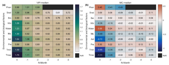
Figure 3.
PLSR–based significance index VIP (a) and correlation index MC (b) statistics between SOS and environmental and biological factors in the Northern Hemisphere. The horizontal coordinate is the preseason months of SOS. As a special case, the first line shows the preseason phenological variables (Phen); Phen–0, Phen–1, and Phen–2 are the previous year’s start, end, and length of the growing season (SOS, EOS, LOS), respectively. Values in the figure represent the median of all pixels.
When screening for meteorological variables, we found that the response of SOS to climatic factors (Tmax, Tmin, Srad) of neighboring and distant months was reversed (Figure 3b). Preseason duration implies the combined effects of spring and winter climate change on SOS, especially from winter warming. We calculated the preseason durations of each pixel for 19 time periods in 15-year time steps and found significant spatial variability in the preseason vegetation duration (Figure S1 of Supplementary Materials), but fewer regions with significant temporal variability (Figure S2 of Supplementary Materials). The application of the optimal preseason could reduce the sensitivity error caused by the change in the preseason over time.
3.2. Sensitivity of SOS to Preseason Meteorological Factors
The sensitivity statistics for the climatic region and plant type are shown in Figure 4. The SCom value for each biome occurred in the following order: forest > shrub > grassland > farmland > sparse vegetation, with the highest sensitivity in mixed forests (MF) (Figure 4a). SCom is also more sensitive in wet and cool zones than in dry, warm, and cold zones. The cool, temperate, and moist (CTM) zones, where most of the Northern Hemisphere deciduous forests are located, are the most sensitive, and warm, temperate, and dry (WTD) zones dominated by grass and sparse vegetation are the least sensitive (Figure 4b). Overall, SOS in the Northern Hemisphere ecosystem showed the highest sensitivity to Tmax (−0.27), followed by Tmin (−0.20), and SOS showed the weakest sensitivity to Wbi and Srad (−0.07, −0.06). Similar conclusions were reached in the ecosystems of most vegetation types and climatic regions.
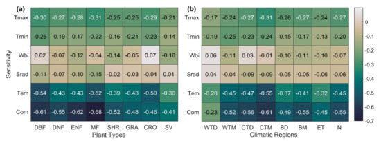
Figure 4.
SOS sensitivity to climate change in different plant types (a) and climatic regions (b) in the Northern Hemisphere during 1982–2014. Values in the figure represent the median of all pixel sensitivity values in different plant types (or climatic regions). The specific meanings of different plant types and climatic regions are shown in Table 1; N stands for the Northern Hemisphere (latitude ≥ 30°).
The spatial distribution of the SOS standardized sensitivity to preseason meteorological factors in the Northern Hemisphere from 1982 to 2014 is shown in Figure S3 of Supplementary Materials. The highest SOS sensitivities to preseason Tmax and Tmin (STmax and STmin) were concentrated in the mid-latitude and non-farming areas. We also found that 19.3% of the pixels showed opposite SOS responses to preseason Tmax and Tmin (Figure S4 of Supplementary Materials). The highest SOS sensitivities to preseason Wbi and Srad (SWbi and SSrad) were mainly distributed at the high latitudes. The proportions of pixels significantly affected by temperature, moisture, and radiation were 88%, 46%, and 29%, respectively; therefore, the spatial distribution of SCom was similar to that of STem (Figure S3c–f of Supplementary Materials). The spatial distribution of each sensitivity’s contribution to SCom (Figure 5d) also shows that STem limits SCom in most pixels of the mid-latitudes, whereas SWbi and SSrad are the dominant drivers of SCom at high latitudes and high elevations. SCom in the Northern Hemisphere was dominated by STem, SWbi, and SSrad from 1982 to 2014, contributing 74.9%, 15.7%, and 9.4%, respectively.
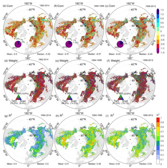
Figure 5.
Spatial distribution of SCom (a–c), weights of STem, SWbi, SSrad (d–f), and decision coefficients (R2) of SOS based on PLSR (g–i) for the periods of the study (1982–2014), rapid warming (1984–1998), and interrupted warming (1998–2012). The four sections of the pie chart in a clockwise direction represent the proportion of pixels with significant positive, positive, negative, and significant negative trends.
3.3. Temporal and Spatial Characteristics of SOS Sensitivity to Preseason Climatic Factors
We calculated the sensitivity of each pixel over 19 periods from 1982 to 2014 using a time window of 15 years. The spatial distribution of SCom varied significantly between the period of rapid warming (1984–1998) and interrupted warming (1998–2012), with the proportion of significantly negative sensitive pixels decreasing from 81% to 76%. The proportion of pixels in which STem, SWbi, and SSrad dominated SCom was 66.8%, 19.0%, and 14.2% during the rapid warming period, respectively, which changed to 61.6%, 22.2%, and 16.1% during the warming interruption. The region in which sensitivity was dominated by Wbi and Srad expanded (Figure 5b,c,e,f).
We observed obvious spatial heterogeneity in the time-varying sensitivity trends (Figure 6 and Figure S5). A total of 39.5% of pixels showed significant changes in SCom (22.2% decrease, 17.3% increase), whereas 53.3% of pixels showed a decreasing trend in the Northern Hemisphere (Figure 6f). The trends in single-factor sensitivity and integrated sensitivity are not spatially consistent, even for the STem that contributes the most to SCom (Figure 6e,f). The statistical results for different climatic zones (Figure S5a of Supplementary Materials) showed that a greater proportion of pixels exhibited reduced sensitivity in cold/moist climates compared with warm/dry climates (WTM = 52.8% > WTD = 46.6%, CTM = 52.8% > CTD = 46.8%, BM = 56.0% > BD = 52.1%, ET = 54.0%). The proportion of pixels with reduced sensitivity was greatest in shrubs (SHR = 57.0%) among all vegetation types (Figure S5b of Supplementary Materials). In terms of temporal trends in the median sensitivity of all pixels in the Northern Hemisphere over 19 time periods (Figure S6 of Supplementary Materials), the sensitivity of SOS to preseason Com, Tmax, Tmin, and Tem was significantly reduced. The sensitivity to preseason Wbi showed a tendency to first decrease and then increase, whereas the opposite was true for preseason Srad, although there were no significant changes. However, the proportion of pixels dominated by SSrad and SWbi in SCom increased significantly with time.
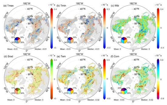
Figure 6.
Spatial distribution of SOS sensitivity trends (Sen’s slope) to climate factors in the Northern Hemisphere over 19 periods with a time step of 15 years during 1982–2014. The dotted regions indicate significant changes in sensitivity (|Z| > 1.95), and the trend in units of ‘/10 a’, a is the abbreviation for annual. The four sections of the pie chart in a clockwise direction represent the proportion of pixels with significant positive, positive, negative, and significant negative trends.
3.4. Effectiveness Evaluation of the Standardized SOS Sensitivity Index
The correlation between the standardized sensitivity index and the SD index (Figure S7 of Supplementary Materials) in most climate regions and plant types is expressed as Com > Tem > Tmax > Tmin > Srad > Wbi. That is, the comprehensive sensitivity index was superior to the single-factor sensitivity index and showed stronger applicability in boreal moist, polar alpine climate regions (BM = −0.60, ET = −0.61) and deciduous needleleaf forests (DNF = −0.67).
3.5. Drivers of the Spatial Pattern of SCom
Several factors affected the spatial pattern of SCom in the Northern Hemisphere from 1982 to 2014 (Figure 7). The spatial pattern was most strongly influenced by the NDVI (VIP = 1.17, MC = 0.05). Moreover, earlier SOS dates corresponded to higher sensitivities (MC = −0.02). SOS sensitivity increased with digital elevation model altitude (DEM, MC = 0.04) and decreased with latitude (LAT, MC = −0.02); the effects of LAT on the spatial distribution of sensitivity were significant (VIP = 1.11). Tmin was the dominant climatic control on the spatial pattern of SCom (VIP = 1.14, MC = −0.014), followed by Tmax (VIP = 1.12, MC = −0.004). Wbi had the weakest effect on the spatial pattern of sensitivity (VIP = 0.48); none of the rates of change of climatic factors had a significant effect on the sensitivity spatial pattern (VIP < 1). However, owing to the complexity of climate and land cover, the impacts of the different drivers on sensitivity were not consistent across different climate regions (Figure S8 of Supplementary Materials).
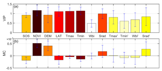
Figure 7.
Driving force analysis of the spatial pattern of SCom in the Northern Hemisphere based on PLSR. Mean values of variable importance in the projection (VIP−a) and mean values of the standardized model regression coefficient (MC−b) for different factors over 19 time periods, 1982−2014.
The influence of various driving factors affecting the spatial pattern of sensitivity changed in response to the slowing down of climate warming (Figure S9 of Supplementary Materials). The influence of biological factors (SOS and NDVI) showed a weakening trend from 1982 to 2014. The influence of DEM first increased and then decreased, while the influence of LAT continued to increase. The impact of spring temperature (Tmax, Tmin) on the spatial distribution of SCom first increased and then decreased. The effect of Wbi showed a decreasing trend, whereas Srad showed the opposite trend. The influences of Tmax, Wbi, and Srad on the spatial distribution of SCom reversed over time (positive and negative MC), which affected the spatial variability of sensitivity. The influence of the climate tendency rate (Tmax’, Tmin’, Wbi’, Srad’) on the spatial pattern of SCom has weakened in recent years.
3.6. Drivers of the Temporal Characteristics of SCom
Biological factors had a stronger effect on the temporal variability of SCom than did climate change (Figure 8). SOS with the maximum VIP value was the dominant driver of the temporal variability of SCom in the Northern Hemisphere, followed by spring temperatures (Tems) and Wbi. Winter temperatures (Temw) and Srad had the weakest influence. The importance of Wbi on the temporal variability of SCom was greater in the arid zones (WTD and CTD) (Figure 8a). According to the spatial distribution of the drivers influencing the temporal variation of SCom (Figure S10 of Supplementary Materials), regions significantly affected by SOS and climate factors were not concentrated. The proportion of pixels showing positive and negative influences on sensitivity for each driving factor in the different climate regions was relatively balanced at ~50% and did not exceed 57.5% (Figure 8b). Considering climate alone, the pixel proportions in which Tem, Wbi, and Srad dominated the temporal variability of SCom in the Northern Hemisphere were 51.6% (Tems = 25.5%, Temw = 26.1%), 26.1%, and 22.3%, respectively. The pixel proportions dominated by Wbi in arid (WTD and CTD) and cold (BD, BM, ET) areas were >25%, and Srad performed best in wet and ET climates (Figure 8c). Our results suggest that temperature change is the dominant climatic control on the temporal variability of SOS sensitivity, with important contributions from water balance and radiation.
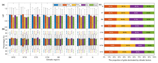
Figure 8.
Statistics on the drivers influencing the temporal variability of SCom in different climatic regions and the Northern Hemisphere, including (a) the average VIP value of each driving factor in each climate region, and (b) the standardized regression coefficient (MC) of the PLSR between climatic variables/SOS and SCom. Bars above and below 0 represent percentage of positive and negative correlations, respectively. The colored sections indicate the percentages of significant correlations at VIP ≥ 1. (c) The proportion of pixels in which climatic variables dominate the temporal change in sensitivity.
Most notably, the effects of spring and winter warming on the temporal variability of sensitivity in different regions of the Northern Hemisphere were superimposed or offset. The proportions of pixels where spring/winter warming jointly promoted and inhibited sensitivity were 23.7% and 23.3%, respectively, whereas 53.1% of pixels showed the opposite effect from spring/winter warming (Figure S11a of Supplementary Materials). The proportion of pixels where spring/winter warming had an opposite effect on sensitivity increased with increasing latitude and decreasing temperature in dry climate regions (WTD = 53.0%, CTD = 53.7%, BD = 58.1%). However, the opposite trend was observed in humid regions (WTM = 51.2%, CTM = 50.4%, BM = 48.8%). In addition, the aforementioned results also showed that the proportion of the asymmetric response of SCom to spring/winter temperature changes was smaller in the humid zone than that in the dry zone. This indicate that more moisture might mitigate the asymmetric response of SCom to spring/winter warming (Figure S11b of Supplementary Materials).
4. Discussion
4.1. Rationality of the Standardized SOS Sensitivity Index and Its Evaluation Results
Both existing studies [18,51,52,53] and the present study showed an asymmetric effect of daytime and nighttime (spring and winter) warming on SOS. However, this asymmetry has rarely been considered in previous SOS sensitivity studies [23,24,33,37,54,55]. Biological and environmental factors combine to regulate the SOS. Interactions between phenological events in spring and autumn may change the phenological response to ongoing climate warming [10], and interspecies interactions may affect SOS [56]. Our results showed that preseason EOS and LOS significantly affect the SOS. Studies have shown that changes in SOS sensitivity to temperature are associated with preseason duration [16,33]. For the aforementioned facts, we constructed a composite sensitivity index to characterize the complex response of spring phenology to climate change (Tmax, Tmin, Wbi, Srad). The effects of the previous year’s phenology (EOS, LOS) and optimal preseason duration were incorporated in the calculation process to exclude the effects of non- meteorological factors on the sensitivity index. The results demonstrated that the composite index was superior to the single-factor index in expressing the influence of SOS due to climate change. Temperature, especially the preseason Tmax, is considered to be the main controlling factor for SOS, as warmer temperature breaks the ecodormancy earlier with global warming [10,51,57]; our results also show that SOS sensitivity to Tmax is highest in the Northern Hemisphere ecosystems and most vegetation types and climate type ecosystems, followed by Tmin. However, we also found that SOS changes were dominated by moisture and radiation in 15.7% and 9.4% of the grid points, respectively. The control of SOS by moisture and radiation can be explained by their indirect effect on the thermal demand of SOS [10]. The interaction between radiation, temperature, and water affects the sensitivity of SOS to climate change [17,25]. SCom can reflect the comprehensive impact of climate change (including changes in light, temperature, and water and their interactions) on SOS.
4.2. Driving Force Analysis of the Spatial Distribution of SCom
The combined interaction between climate characteristics, climate tendency, and biological and geographical factors influences the spatial pattern of sensitivity. However, few studies have examined these factors together to identify the dominant drivers for the spatial distribution of SOS sensitivity. STem was the highest in the forests [55]. SOS in warmer locations of the Northern Hemisphere was found to be less responsive to climate change, and STem increased with altitude (cold climate) [33]. Wang et al. [23] found that the temperature sensitivity decreased with increasing spring temperature. Moreover, vegetation at lower latitudes (or with earlier SOS) was found to be more sensitive to changes in spring temperature [37,54]. Climatic tendency is highly correlated with SOS [20]. The findings of this study are consistent with these observations. In addition, we found that the multi-year average NDVI (an index reflecting the status of surface vegetation cover) had the greatest influence on the spatial distribution of SCom. SCom decreased with increasing latitude (or decreasing temperature) in this study, despite warmer regions (lower latitudes) showing lower sensitivity. This may be due to the importance of vegetation coverage (NDVI) on the spatial distribution of sensitivity, with higher sensitivity at higher coverage. Sparse vegetation, grasslands, and tundra dominate the high latitudes, high altitudes, and cold regions; this prevents SOS from closely tracking changes in temperature to avoid frost risks [58].
The spatial distribution of SCom showed diametrically opposed responses to drivers in different climatic regions (Figure S5 of Supplementary Materials) attributable to the regional characteristics of vegetation and climate types in the Northern Hemisphere, which might also be due to the interaction of hydrothermal conditions to influence the distribution of SOS sensitivity [25]. With the exception of LAT and Srad, the influence of biological factors (SOS, NDVI), climate characteristics (Tmax, Tmin, Wbi), climate trend rate (Tmax’, Tmin’, Wbi’, Srad’), and geographical factors (DEM) on the spatial pattern of sensitivity has weakened in recent years (Figure S6 of Supplementary Materials). The reasons for this phenomenon are as follows: First, the vegetation and the communities in which they are located have adapted to climate warming [31,56]. Furthermore, the rate of warming has decreased, resulting in no trends in SOS during the global warming hiatus [31,56]. Finally, a faster rate of warming at higher altitudes has led to SOS at different altitudes becoming more uniform [15,59].
4.3. Driving Force Analysis of the Temporal Variability of SCom
According to global average surface temperature data, a global warming interruption occurred between 1998 and 2012 [60,61]. To explore the effect of this warming slowdown on SOS sensitivity, we analyzed the temporal variability and dominant drivers of SOS sensitivity using a time window of 15 years. The simulated effect (R2 = 0.57) of preseason climate change and phenology on SOS dynamics was significantly enhanced at the 15-year time step (Figure 4g,h,j) relative to the 33-year time window (R2 = 0.40), which allowed us to obtain more accurate SOS sensitivity, as the SOS response to preseason climate change (especially temperature change) is nonlinear [29].
SOS sensitivity to climate warming generally shows a decreasing trend in the Northern Hemisphere [29]. The present study also showed a significant decreasing trend in the median of all pixels SCom (or STem) in the Northern Hemisphere. However, we found that only 53.3% of the pixels showed a decrease in SCom; 22.2% were statistically significant (Figure 5 and Figure S2a). This may suggest that the decrease in the sensitivity trend exceeded the increase on the pixel scale. The significant reduction in SOS sensitivity in a small proportion of vegetation leads to a decreasing trend of SCom (or STem) in the Northern Hemisphere, with vegetation in wetter/cooler climate zones and shrubs contributing more to the decrease in sensitivity. In all climate regions other than WTM, we found that biological factors (SOS) exert more influence on the temporal variability of SOS sensitivity relative to each climatic factor (Tems, Temw, Wbi, Srad), suggesting that vegetation autonomously regulates SOS to adapt to climate change [31]. Vegetation adaptation is the most important factor influencing temporal variation in SCom.
Temperature may be an important climate driver dominating temporal changes in sensitivity (5.16% of the pixels). Strong uncertainty remains in the main climatic factors that driver the temporal variability of sensitivity. In different climatic regions and the Northern Hemisphere, the proportion of positive and negative responses of sensitivity to various driving factors (biological and climatic) was relatively balanced (Figure 7b). This may be due to the spatial heterogeneity (Figure 5 and Figure S2) of the sensitivity variation (only 53.3% of the pixels showed a decrease in sensitivity), or the asymmetric response of SCom to spring/winter warming (53.1% of pixels showed the opposite effect). More likely, it is due to the complex interaction of drivers [10]. For example, radiation showed clear time-varying characteristics [62], and the proportion of pixels dominated by radiation reached 22.3% in this study. Moreover, strong solar radiation in spring causes snow to melt, leading to higher temperatures in the soil relative to the atmosphere. The sensitivity of SOS may be affected by the influx of snowmelt water into partially frozen soils, as this promotes root activity before temperatures reach 0 °C [63]. The effect of Wbi on the temporal variability of SCom was greater than or equal to the effect of Tems in arid and cold climate regions. Water shortage in these regions is the dominant limiting factor in the development of spring phenology [64]. We also found that more moisture might mitigate the asymmetric response of SCom to spring/winter warming. Srad and Temw showed weaker influences on the temporal variability of sensitivity relative to Wbi and Tems; however, the proportion of pixels in which the temporal sensitivity was dominated by Temw still reached 26.1%. Studies have shown that warming in winter and early spring shortens the cold storage period, which reduces sensitivity, as the cold storage requirements of certain plant types are not met [65]. Although the response of sensitivity to climatic factors is complex, the main driving factors still have different emphases in different climatic regions.
4.4. Limitations
As the four methods to estimate SOS were based on satellite data, some uncertainties may arise due to resolution and data quality limitations. Moreover, although we selected pixels with no significant change in land cover type for statistical analysis, they may still include some impacts from human activity. We studied the spatial and temporal patterns of spring phenology sensitivity and analyzed the relative importance of each driving factor to the spatial and temporal distribution of sensitivity. However, we do not understand the underlying causes and ecological processes that lead to these patterns. Meteorological and phenological observations with higher spatio–temporal resolution and manipulatable physiological experiments can further our understanding of the underlying mechanisms of the SOS response to climate change.
5. Conclusions
We applied the PLSR method as the core algorithm and used meteorological and NDVI-extracted phenological data to screen the most suitable biological and climatic indicators affecting SOS in the Northern Hemisphere. We then constructed a standardized SOS sensitivity index for climate change based on the optimal preseason duration of the climatic indicators. The index can determine the weight and direction of individual climate factors as well as their combined effects on SOS. Based on the sensitivity evaluation results, we analyzed the spatial and temporal characteristics of SOS sensitivity and its dominant drivers in the Northern Hemisphere from 1982 to 2014.
This study showed that the combined sensitivity of SOS to climate change (SCom) is most influenced by pre-season temperature sensitivity. However, because of the asymmetric response of SOS to Tmax/Tmin and the non-negligible moderating effect of Wbi and Srad on SOS, SCom was more effective in expressing the effect of climate change on SOS compared with the single climatic factor. Vegetation cover (or type) was the dominant factor influencing the spatial pattern of SOS sensitivity, followed by spring temperature (Tmin > Tmax); the weakest was Wbi. Forests had the highest SCom absolute values. In recent years, a significant decrease in the sensitivity of some vegetation has led to a decreasing trend of sensitivity in the Northern Hemisphere, with vegetation in wetter/cooler climate zones and shrubs contributing more to the decrease in SCom. Biological factors (vegetation adaptation) exerted a greater influence on the temporal variability of SOS sensitivity relative to each climatic factor (Tems, Temw, Wbi, Srad). Although temperature remains the main climatic factor driving temporal changes in SCom, the effects were asymmetric between spring and winter. More moisture might mitigate the asymmetric response of SCom to spring/winter warming. Despite the complex response of sensitivity to climate change, the dominant factors in different climatic regions still have different emphases.
Identifying systematic differences in phenological climate sensitivity would facilitate the development of indicators and estimates of vulnerability for conservation and national adaptation programs [32]. The performance of the current phenological models is unsatisfactory [10]. The quantitative evaluation of sensitivity and driving force analysis of SOS in this study provides not only a new method for identifying the combined sensitivity of springtime phenology to climate change but also a basis for the construction of better phenological models to improve phenological prediction performance.
Supplementary Materials
The following are available online at https://www.mdpi.com/article/10.3390/rs13101972/s1. Figure S1: Average optimal preseason duration of Tmax (a), Tmin (b), Wbi (c), Srad (d) for SOS in the north during 1982–2014; Figure S2: Spatial distribution of optimal preseason duration trends in SOS on Tmax (a), Tmin (b), Wbi (c), Srad (d) in the north during 1982–2014; Figure S3: Spatial distribution of SOS sensitivity to Tmax (a), Tmin (b), Wbi (c), Srad (d), Tem (e), and Com (f); Figure S4: Asymmetric effects of preseason Tmax and Tmin on SOS; Figure S5: Statistics of the time-varying trends in SOS sensitivity to climate factors in different climatic regions (a) and plant types (b); Figure S6.: Temporal changes in SOS sensitivity to climate factors in the north (a–e) and the proportion of climate factors dominating sensitivity (f); Figure S7: Correlation between the standardized sensitivity index and SD index in different climate regions (a) and plant types (b); Figure S8: Driving force analysis of the spatial pattern of SCom during 1982–2014 (on a 33-year time scale) in different climatic regions and the Northern Hemisphere based on PLSR; Figure S9: Changes in the influence of drivers on the spatial pattern of SCom in the Northern Hemisphere during 1982–2014 (on a 15-year time scale); Figure S10: The spatial distribution of the driving forces influencing the temporal variability of SCom in the Northern Hemisphere; Figure S11: Effects of asymmetric warming in spring and winter on the temporal variation of SCom.
Author Contributions
All authors contributed meaningfully to this study. K.L., J.Z. designed the research; C.W., Q.S. performed the research, analyzed the data; G.R., Z.T., X.L. provided methodology support and revised the paper; K.L. drafted the manuscript, and all authors reviewed and edited the writing. All authors have read and agreed to the published version of the manuscript.
Funding
This study was supported by the National Key R&D Program of China (2019YFD1002201), the National Natural Science Foundation of China (41877520), the Science and Technology Development Planning of Jilin Province (20190303018SF), and the Changchun Key Scientific and Technology Program (19SS007).
Institutional Review Board Statement
Not applicable.
Informed Consent Statement
Not applicable.
Data Availability Statement
Not applicable.
Conflicts of Interest
The authors declare no conflict of interest.
Abbreviations
| Aet | Actual evapotranspiration |
| CCI | European Space Agency’s Climate Change Initiative |
| DEM | Digital elevation model altitude |
| EOS | End of the growing season |
| IPCC | Intergovernmental Panel on Climate Change |
| JRC | Joint Research Centre |
| LAT | Latitude |
| LC | Land Cover |
| LOS | Lengths of the growing season |
| MC | The standardized model regression coefficient |
| MK | Mann–Kendall |
| Ms | Melting snow water equivalent |
| NDNI | Normalized difference vegetation index |
| PLSR | Partial least squares regression |
| Pre | Accumulated precipitation |
| SCom | Combined sensitivity of SOS to climate change |
| SD | Standard deviation |
| Sm | Soil moisture |
| SOS | Start of growing season (or spring green-up date) |
| Srad | Radiation (or Downward shortwave flux at the surface) |
| STem/STmax/STmin/SWbi/SSrad | Sensitivity of SOS to preseason Tem/Tmax/Tmin/Wbi/Srad |
| Swe | Snow water equivalent |
| Tem | Air temperature |
| Tems/Temw | Spring/Winter temperature |
| Tmax/Tmin | daytime/night temperature (or Maximum/Minimum temperature) |
| Tmin’/Tmax’/Wbi’/Srad’ | Climate tendency rate of Tmin/Tmax/Wbi/Srad |
| TS | Then–Sen |
| VIP | Variable importance in the projection |
| Wbi | Water balance |
References
- Leblans, N.I.; Sigurdsson, B.D.; Vicca, S.; Fu, Y.; Penuelas, J.; Janssens, I.A. Phenological responses of Icelandic subarctic grasslands to short-term and long-term natural soil warming. Glob. Chang. Biol. 2017, 23, 4932–4945. [Google Scholar] [CrossRef] [PubMed]
- Renner, S.S.; Zohner, C.M. Climate Change and Phenological Mismatch in Trophic Interactions Among Plants, Insects, and Vertebrates. Annu. Rev. Ecol. Evol. Syst. 2018, 49, 165–182. [Google Scholar] [CrossRef]
- Richardson, A.D.; Keenan, T.F.; Migliavacca, M.; Ryu, Y.; Sonnentag, O.; Toomey, M. Climate change, phenology, and phenological control of vegetation feedbacks to the climate system. Agric. For. Meteorol. 2013, 169, 156–173. [Google Scholar] [CrossRef]
- Xu, X.; Riley, W.J.; Koven, C.D.; Jia, G.; Zhang, X. Earlier leaf-out warms air in the north. Nat. Clim. Chang. 2020, 10, 370–375. [Google Scholar] [CrossRef]
- Garonna, I.; de Jong, R.; Schaepman, M.E. Variability and evolution of global land surface phenology over the past three decades (1982–2012). Glob. Chang. Biol. 2016, 22, 1456–1468. [Google Scholar] [CrossRef] [PubMed]
- Yang, L.H.; Rudolf, V.H.W. Phenology, ontogeny and the effects of climate change on the timing of species interactions. Ecol. Lett. 2010, 13, 1–10. [Google Scholar] [CrossRef]
- Zhou, X.; Geng, X.; Yin, G.; Hänninen, H.; Hao, F.; Zhang, X.; Fu, Y.H. Legacy effect of spring phenology on vegetation growth in temperate China. Agric. For. Meteorol. 2020, 281, 107845. [Google Scholar] [CrossRef]
- Ma, X.; Huete, A.; Moran, S.; Ponce-Campos, G.; Eamus, D. Abrupt shifts in phenology and vegetation productivity under climate extremes. J. Geophys. Res. Biogeosci. 2015, 120, 2036–2052. [Google Scholar] [CrossRef]
- Wang, S.; Zhang, B.; Yang, Q.; Chen, G.; Yang, B.; Lu, L.; Shen, M.; Peng, Y. Responses of net primary productivity to phenological dynamics in the Tibetan Plateau, China. Agric. For. Meteorol. 2017, 232, 235–246. [Google Scholar] [CrossRef]
- Piao, S.; Liu, Q.; Chen, A.; Janssens, I.A.; Fu, Y.; Dai, J.; Liu, L.; Lian, X.; Shen, M.; Zhu, X. Plant phenology and global climate change: Current progresses and challenges. Glob. Chang. Biol. 2019, 25, 1922–1940. [Google Scholar] [CrossRef]
- Wang, X.; Wu, C.; Zhang, X.; Li, Z.; Liu, Z.; Gonsamo, A.; Ge, Q. Satellite-observed decrease in the sensitivity of spring phenology to climate change under high nitrogen deposition. Environ. Res. Lett. 2020, 15, 094055. [Google Scholar] [CrossRef]
- Shen, M.; Piao, S.; Cong, N.; Zhang, G.; Jassens, I.A. Precipitation impacts on vegetation spring phenology on the Tibetan P lateau. Glob. Chang. Biol. 2015, 21, 3647–3656. [Google Scholar] [CrossRef] [PubMed]
- Garonna, I.; de Jong, R.; Stöckli, R.; Schmid, B.; Schenkel, D.; Schimel, D.; Schaepman, M.E. Shifting relative importance of climatic constraints on land surface phenology. Environ. Res. Lett. 2018, 13, 24025. [Google Scholar] [CrossRef]
- Zhao, M.; Peng, C.; Xiang, W.; Deng, X.; Tian, D.; Zhou, X.; Yu, G.; He, H.; Zhao, Z. Plant phenological modeling and its application in global climate change research: Overview and future challenges. Environ. Rev. 2013, 21, 1–14. [Google Scholar] [CrossRef]
- Chen, X.; An, S.; Inouye, D.W.; Schwartz, M.D. Temperature and snowfall trigger alpine vegetation green-up on the world’s roof. Glob. Chang. Biol. 2015, 21, 3635–3646. [Google Scholar] [CrossRef]
- Liu, Q.; Fu, Y.H.; Zhu, Z.; Liu, Y.; Liu, Z.; Huang, M.; Janssens, I.A.; Piao, S. Delayed autumn phenology in the Northern Hemisphere is related to change in both climate and spring phenology. Glob. Chang. Biol. 2016, 22, 3702–3711. [Google Scholar] [CrossRef]
- Chen, L.; Huang, J.G.; Ma, Q.; Hänninen, H.; Rossi, S.; Piao, S.; Bergeron, Y. Spring phenology at different altitudes is becoming more uniform under global warming in Europe. Glob. Chang. Biol. 2018, 24, 3969–3975. [Google Scholar] [CrossRef]
- Deng, G.; Zhang, H.; Guo, X.; Shan, Y.; Ying, H.; Rihan, W.; Li, H.; Han, Y. Asymmetric Effects of Daytime and Nighttime Warming on Boreal Forest Spring Phenology. Remote Sens. 2019, 11, 1651. [Google Scholar] [CrossRef]
- He, Z.; Du, J.; Chen, L.; Zhu, X.; Lin, P.; Zhao, M.; Fang, S. Impacts of recent climate extremes on spring phenology in arid-mountain ecosystems in China. Agric. For. Meteorol. 2018, 260, 31–40. [Google Scholar] [CrossRef]
- Wang, X.; Xiao, J.; Li, X.; Cheng, G.; Ma, M.; Zhu, G.; Altaf Arain, M.; Andrew Black, T.; Jassal, R.S. No trends in spring and autumn phenology during the global warming hiatus. Nat. Commun. 2019, 10, 2389. [Google Scholar] [CrossRef]
- Yang, B.; He, M.; Shishov, V.; Tychkov, I.; Vaganov, E.; Rossi, S.; Ljungqvist, F.C.; Bräuning, A.; Grießinger, J. New perspective on spring vegetation phenology and global climate change based on Tibetan Plateau tree-ring data. Proc. Natl. Acad. Sci. USA 2017, 114, 6966–6971. [Google Scholar] [CrossRef] [PubMed]
- Keenan, T.F.; Richardson, A.D.; Hufkens, K. On quantifying the apparent temperature sensitivity of plant phenology. New Phytol. 2020, 225, 1033–1040. [Google Scholar] [CrossRef] [PubMed]
- Wang, T.; Ottlé, C.; Peng, S.; Janssens, I.A.; Lin, X.; Poulter, B.; Yue, C.; Ciais, P. The influence of local spring temperature variance on temperature sensitivity of spring phenology. Glob. Chang. Biol. 2014, 20, 1473–1480. [Google Scholar] [CrossRef] [PubMed]
- Wang, C.; Cao, R.; Chen, J.; Rao, Y.; Tang, Y. Temperature sensitivity of spring vegetation phenology correlates to within-spring warming speed over the Northern Hemisphere. Ecol. Indic. 2015, 50, 62–68. [Google Scholar] [CrossRef]
- Du, J.; He, Z.; Piatek, K.B.; Chen, L.; Lin, P.; Zhu, X. Interacting effects of temperature and precipitation on climatic sensitivity of spring vegetation green-up in arid mountains of China. Agric. For. Meteorol. 2019, 269–270, 71–77. [Google Scholar] [CrossRef]
- Marchin, R.M.; Salk, C.F.; Hoffmann, W.A.; Dunn, R.R. Temperature alone does not explain phenological variation of diverse temperate plants under experimental warming. Glob. Chang. Biol. 2015, 21, 3138–3151. [Google Scholar] [CrossRef]
- Flynn, D.F.B.; Wolkovich, E.M. Temperature and photoperiod drive spring phenology across all species in a temperate forest community. New Phytologist. 2018, 219, 1353–1362. [Google Scholar] [CrossRef] [PubMed]
- Shen, M.; Tang, Y.; Chen, J.; Yang, X.; Wang, C.; Cui, X.; Yang, Y.; Han, L.; Li, L.; Du, J.; et al. Earlier-Season Vegetation Has Greater Temperature Sensitivity of Spring Phenology in Northern Hemisphere. PLoS ONE 2014, 9, e88178. [Google Scholar] [CrossRef]
- Fu, Y.H.; Zhao, H.; Piao, S.; Peaucelle, M.; Peng, S.; Zhou, G.; Ciais, P.; Huang, M.; Menzel, A.; Peñuelas, J. Declining global warming effects on the phenology of spring leaf unfolding. Nature 2015, 526, 104–107. [Google Scholar] [CrossRef]
- Jin, Z.; Zhuang, Q.; Dukes, J.S.; He, J.; Sokolov, A.P.; Chen, M.; Zhang, T.; Luo, T. Temporal variability in the thermal requirements for vegetation phenology on the Tibetan plateau and its implications for carbon dynamics. Clim. Chang. 2016, 138, 617–632. [Google Scholar] [CrossRef]
- Peaucelle, M.; Janssens, I.A.; Stocker, B.D.; Descals Ferrando, A.; Fu, Y.H.; Molowny-Horas, R.; Ciais, P.; Peñuelas, J. Spatial variance of spring phenology in temperate deciduous forests is constrained by background climatic conditions. Nat. Commun. 2019, 10, 5310–5388. [Google Scholar] [CrossRef]
- Thackeray, S.J.; Henrys, P.A.; Hemming, D.; Bell, J.R.; Botham, M.S.; Burthe, S.; Helaouet, P.; Johns, D.G.; Jones, I.D.; Leech, D.I. Phenological sensitivity to climate across taxa and trophic levels. Nature 2016, 535, 241–245. [Google Scholar] [CrossRef]
- Güsewell, S.; Furrer, R.; Gehrig, R.; Pietragalla, B. Changes in temperature sensitivity of spring phenology with recent climate warming in Switzerland are related to shifts of the preseason. Glob. Chang. Biol. 2017, 23, 5189–5202. [Google Scholar] [CrossRef] [PubMed]
- Gao, M.; Wang, X.; Meng, F.; Liu, Q.; Li, X.; Zhang, Y.; Piao, S. Three-dimensional change in temperature sensitivity of northern vegetation phenology. Glob. Chang. Biol. 2020, 26, 5189–5201. [Google Scholar] [CrossRef]
- Liu, L.; Liu, L.; Liang, L.; Donnelly, A.; Park, I.; Schwartz, M.D. Effects of elevation on spring phenological sensitivity to temperature in Tibetan Plateau grasslands. Chin. Sci. Bull. 2014, 59, 4856–4863. [Google Scholar] [CrossRef]
- Li, K.; Tong, Z.; Liu, X.; Zhang, J.; Tong, S. Quantitative assessment and driving force analysis of vegetation drought risk to climate change: Methodology and application in Northeast China. Agric. For. Meteorol. 2020, 282, 107865. [Google Scholar] [CrossRef]
- Liu, Q.; Piao, S.; Fu, Y.H.; Gao, M.; Peñuelas, J.; Janssens, I.A. Climatic Warming Increases Spatial Synchrony in Spring Vegetation Phenology Across the Northern Hemisphere. Geophys. Res. Lett. 2019, 46, 1641–1650. [Google Scholar] [CrossRef]
- Abatzoglou, J.T.; Dobrowski, S.Z.; Parks, S.A.; Hegewisch, K.C. TerraClimate, a high-resolution global dataset of monthly climate and climatic water balance from 1958–2015. Sci. Data 2018, 5, 170191. [Google Scholar] [CrossRef] [PubMed]
- Li, W.; MacBean, N.; Ciais, P.; Defourny, P.; Lamarche, C.; Bontemps, S.; Houghton, R.A.; Peng, S. Gross and net land cover changes in the main plant functional types derived from the annual ESA CCI land cover maps (1992–2015). Earth Syst. Sci. Data 2018, 10, 219–234. [Google Scholar] [CrossRef]
- Beck, H.E.; Zimmermann, N.E.; McVicar, T.R.; Vergopolan, N.; Berg, A.; Wood, E.F. Present and future Köppen-Geiger climate classification maps at 1-km resolution. Sci. Data 2018, 5, 180214. [Google Scholar] [CrossRef] [PubMed]
- Jin, J.; Wang, Y.; Zhang, Z.; Magliulo, V.; Jiang, H.; Cheng, M. Phenology Plays an Important Role in the Regulation of Terrestrial Ecosystem Water-Use Efficiency in the Northern Hemisphere. Remote Sens. 2017, 9, 664. [Google Scholar] [CrossRef]
- Studer, S.; Stöckli, R.; Appenzeller, C.; Vidale, P.L. A comparative study of satellite and ground-based phenology. Int. J. Biometeorol. 2007, 51, 405–414. [Google Scholar] [CrossRef]
- Zhang, X.; Friedl, M.A.; Schaaf, C.B.; Strahler, A.H.; Hodges, J.C.F.; Gao, F.; Reed, B.C.; Huete, A. Monitoring vegetation phenology using MODIS. Remote Sens. Environ. 2003, 84, 471–475. [Google Scholar] [CrossRef]
- Yu, H.; Luedeling, E.; Xu, J. Winter and spring warming result in delayed spring phenology on the Tibetan Plateau. Proc. Natl. Acad. Sci. USA 2010, 107, 22151–22156. [Google Scholar] [CrossRef]
- White, M.A.; Thornton, P.E.; Running, S.W. A continental phenology model for monitoring vegetation responses to interannual climatic variability. Glob. Biogeochem. Cycles 1997, 11, 217–234. [Google Scholar] [CrossRef]
- Mateos-Aparicio, G. Partial Least Squares (PLS) Methods: Origins, Evolution, and Application to Social Sciences. Commun. Stat. Theory Methods 2011, 40, 2305–2317. [Google Scholar] [CrossRef]
- Chen, C.; He, B.; Guo, L.; Zhang, Y.; Xie, X.; Chen, Z. Identifying Critical Climate Periods for Vegetation Growth in the Northern Hemisphere. J. Geophys. Res. Biogeosci. 2018, 123, 2541–2552. [Google Scholar] [CrossRef]
- Zhang, Q.; Kong, D.; Shi, P.; Singh, V.P.; Sun, P. Vegetation phenology on the Qinghai-Tibetan Plateau and its response to climate change (1982–2013). Agric. For. Meteorol. 2018, 248, 408–417. [Google Scholar] [CrossRef]
- Li, S.; Yang, S.; Liu, X.; Liu, Y.; Shi, M. NDVI-based analysis on the influence of climate change and human activities on vegetation restoration in the Shaanxi-Gansu-Ningxia Region, Central China. Remote Sens. 2015, 7, 11163–11182. [Google Scholar] [CrossRef]
- Tabari, H.; Somee, B.S.; Zadeh, M.R. Testing for long-term trends in climatic variables in Iran. Atmos. Res. 2011, 100, 132–140. [Google Scholar] [CrossRef]
- Rossi, S.; Isabel, N. Bud break responds more strongly to daytime than night-time temperature under asymmetric experimental warming. Glob. Chang. Biol. 2017, 23, 446–454. [Google Scholar] [CrossRef]
- Suonan, J.; Classen, A.T.; Zhang, Z.; He, J.S. Asymmetric winter warming advanced plant phenology to a greater extent than symmetric warming in an alpine meadow. Funct. Ecol. 2017, 31, 2147–2156. [Google Scholar] [CrossRef]
- Wang, X.; Xiao, J.; Li, X.; Cheng, G.; Ma, M.; Che, T.; Dai, L.; Wang, S.; Wu, J. No Consistent Evidence for Advancing or Delaying Trends in Spring Phenology on the Tibetan Plateau. J. Geophys. Res. Biogeosci. 2017, 122, 3288–3305. [Google Scholar] [CrossRef]
- Wang, H.; Ge, Q.; Dai, Y.; Dai, J. Parameterization of temperature sensitivity of spring phenology and its application in explaining diverse phenological responses to temperature change. Sci. Rep. 2015, 5, srep08833. [Google Scholar] [CrossRef] [PubMed]
- Xu, X.; Riley, W.J.; Koven, C.D.; Jia, G. Observed and simulated sensitivities of spring greenup to preseason climate in northern temperate and boreal regions. J. Geophys. Res. Biogeosci. 2018, 123, 60–78. [Google Scholar] [CrossRef]
- Kopp, C.W.; Cleland, E.E. A range-expanding shrub species alters plant phenological response to experimental warming. PLoS ONE 2015, 10, e139029. [Google Scholar] [CrossRef] [PubMed]
- Piao, S.; Tan, J.; Chen, A.; Fu, Y.H.; Ciais, P.; Liu, Q.; Janssens, I.A.; Vicca, S.; Zeng, Z.; Jeong, S. Leaf onset in the northern hemisphere triggered by daytime temperature. Nat. Commun. 2015, 6, 6911. [Google Scholar] [CrossRef]
- He, Z.; Du, J.; Zhao, W.; Yang, J.; Chen, L.; Zhu, X.; Chang, X.; Liu, H. Assessing temperature sensitivity of subalpine shrub phenology in semi-arid mountain regions of China. Agric. For. Meteorol. 2015, 213, 42–52. [Google Scholar] [CrossRef]
- Vitasse, Y.; Signarbieux, C.; Fu, Y.H. Global warming leads to more uniform spring phenology across elevations. Proc. Natl. Acad. Sci. USA 2018, 115, 1004–1008. [Google Scholar] [CrossRef]
- Fyfe, J.C.; Meehl, G.A.; England, M.H.; Mann, M.E.; Santer, B.D.; Flato, G.M.; Hawkins, E.; Gillett, N.P.; Xie, S.; Kosaka, Y.; et al. Making sense of the early-2000s warming slowdown. Nat. Clim. Chang. 2016, 6, 224–228. [Google Scholar] [CrossRef]
- Medhaug, I.; Stolpe, M.B.; Fischer, E.M.; Knutti, R. Reconciling controversies about the ‘global warming hiatus’. Nature 2017, 545, 41–47. [Google Scholar] [CrossRef]
- Kleidon, A.; Renner, M. A simple explanation for the sensitivity of the hydrologic cycle to surface temperature and solar radiation and its implications for global climate change. Earth Syst. Dynam. 2013, 4, 455–465. [Google Scholar] [CrossRef]
- Yun, J.; Jeong, S.; Ho, C.; Park, C.; Park, H.; Kim, J. Influence of winter precipitation on spring phenology in boreal forests. Glob. Chang. Biol. 2018, 24, 5176–5187. [Google Scholar] [CrossRef] [PubMed]
- Shen, M.; Tang, Y.; Chen, J.; Zhu, X.; Zheng, Y. Influences of temperature and precipitation before the growing season on spring phenology in grasslands of the central and eastern Qinghai-Tibetan Plateau. Agric. For. Meteorol. 2011, 151, 1711–1722. [Google Scholar] [CrossRef]
- Asse, D.; Chuine, I.; Vitasse, Y.; Yoccoz, N.G.; Delpierre, N.; Badeau, V.; Delestrade, A.; Randin, C.F. Warmer winters reduce the advance of tree spring phenology induced by warmer springs in the Alps. Agric. For. Meteorol. 2018, 252, 220–230. [Google Scholar] [CrossRef]


Publisher’s Note: MDPI stays neutral with regard to jurisdictional claims in published maps and institutional affiliations. |
© 2021 by the authors. Licensee MDPI, Basel, Switzerland. This article is an open access article distributed under the terms and conditions of the Creative Commons Attribution (CC BY) license (https://creativecommons.org/licenses/by/4.0/).