Efficient Rotational Angular Velocity Estimation of Rotor Target via Modified Short-Time Fractional Fourier Transform

Abstract

As a special micro-motion feature of rotor target, rotational angular velocity can provide a discriminant basis for target classification and recognition. In this paper, the authors focus on an efficient rotational angular velocity estimation method of the rotor target is based on the combination of the time–frequency analysis algorithm and Hough transform. In order to avoid the problems of low time–frequency resolution and cross-term interference in short-time Fourier transform and Wigner–Ville distribution algorithm, a modified short-time fractional Fourier transform (M-STFRFT) is proposed to obtain the time-FRFT domain (FRFD)-frequency spectrum with the highest time–FRFD–frequency resolution. In particular, an orthogonal matching pursuit (OMP)-based algorithm is proposed to reduce the computational complexity when estimating the matched transform order in the proposed M-STFRFT algorithm. Firstly, partial transform order candidates are selected randomly from the complete candidates. Then, a partial entropy vector corresponding to partial transform order candidates is calculated from the FRFT results and utilized to reconstruct the complete entropy vector via the OMP algorithm, and the matched transform order can be estimated by searching minimum entropy. Based on the estimated matched transform order, STFRFT is performed to obtain the time–FRFD–frequency spectrum. Moreover, Hough transform is employed to obtain the energy accumulation spectrum, and the micro-Doppler parameter of rotational angular velocity can be estimated by searching the peak value from the energy accumulation spectrum. Both simulated data and measured data collected by frequency modulated continuous wave radar validate the effectiveness of the proposed algorithm.

1. Introduction

The micro-Doppler (m-D) effect is a frequency modulation (FM) induced by the micro-motion [1,2,3], including rotation, vibration, precession, and nutation, which widely exists in many objects or their structures, such as rotors of a helicopter, warhead in mid-phase, running vehicle engines, and so on. As the m-D effect can provide abundant information about a target’s motion, it has attracted extensive application in target imaging, detection, recognition, and classification. The m-D effect of radar echo signals usually behaves as the nonlinear and time-varying frequency in a narrow frequency band, which is related to the target structure, micro-motion property, and the carrier frequency of the transmitting signal [4,5]. This valuable relationship may help realize micro-motion parameter estimation based on m-D distribution signatures in the time–frequency domain.

By contrast with the Fourier transform (FT), the time–frequency analysis class transforms not only provide joint distribution information in the time domain and frequency domain, but also clearly describe the relationship between signal frequency and time. Therefore, they are widely employed in micro-motion parameter estimation [6,7]. Generally, time-frequency analysis class transforms can be divided into two categories: (1) linear time–frequency transform, such as short-time Fourier transform (STFT) and continuous wavelet transform (CWT) [8]; (2) nonlinear time–frequency transform, including Wigner–Ville distribution (WVD) and Cohen class distribution [9].

As a typical algorithm of linear time–frequency transform, STFT has received wide attention and been applied in several fields, such as the instantaneous frequency estimation [10] and the enhancing of spectral resolution [11]. Although these methods have achieved effective performance in parameter estimation and low computational complexity, respectively, the STFT algorithm still suffers from poor concentration [12]. WVD, as the most basic Cohen class bilinear time–frequency distribution, was first proposed by Wigner in quantum mechanics, and then was first applied to signal analysis by Ville [13]. It not only essentially distributes the signal energy in the time–frequency plane, but also has a good time–frequency resolution. However, the existence of cross-term makes it have false information when analyzing multicomponent signals [14,15]. In view of this problem, several studies have been in-depth conducted by many scholars, such as pseudo Wigner–Ville distribution (PWVD) [16] and reassigned smoothed pseudo Wigner–Ville distribution (RSPWVD) [17]. Since Hough transform can map the time–frequency distribution on the parameter space through achieving energy accumulation along the Doppler frequency change rule of the signal, it is usually used to estimate the micro-Doppler parameters from the time–frequency domain spectrum. The Hough transform was combined with STFT, WVD, PWVD, and RSPWVD for parameter estimation in the Hough–STFT algorithm [18], Hough–WVD algorithm [15], Hough–PWVD algorithm [6], and Hough–RSPWVD algorithm [19], respectively. In these algorithms, the correct micro-Doppler parameters can be estimated from parameter candidate sets by finding the location of the maximal Hough integration in these algorithms. Although the time–frequency analysis algorithms mentioned above can realize the estimation of micro-Doppler parameters, they are still plagued by low time–frequency resolution and cross-term interference.

The fractional Fourier transform (FRFT) [20,21] is a generalization of the Fourier transform with an additional transform order parameter and was first proposed by Victor Namias in 1980 [22]. Because of the best energy concentration in the FRFT domain (FRFD) with a certain order in terms of the chirp signal, several implementations and fast computational algorithms of FRFT have been derived in recent years; also, they are widely applied in radar signal processing. Inspired by sparse Fourier transform (SFT) [23] and Pei’s discrete FRFT [24], a novel sparse discrete FRFT (SDFRFT) was proposed by Liu et al. to reduce the computational complexity when dealing with large data sets, which are sparsely represented in the FRFD [25]. Chen et al. proposed adaptive sparse fractional Fourier transform algorithm and used it in fast and refined processing of radar maneuvering target [26]. These algorithms implement FRFT and improve the effectiveness of FRFT through sparse representation. However, in the essential stage of the matched transform order estimation, these algorithms still use the traditional search method or the combination of polynomial phase transform and accurate search method, which are more time-consuming and will increase the computational complexity. However, the FRFT only reveals the signal energy distribution in FRFD under the matched transform order and fails to show the changes of FRFD-frequency with time. In order to introduce the FRFT to the traditional time–frequency representation, the short-time fractional Fourier transform (STFRFT) was proposed [27,28], which draws the process of windowing in STFT into FRFT, to clarify the instantaneous FRFD-frequency and display the time and FRFD information jointly in the time-FRFD plane. With higher concentration and no interference of cross-term, the STFRFT could provide tight support for the signals and eliminate the interference [29,30]. An effective algorithm based on STFRFT is proposed for target detection and m-D signal extraction, in which the radar echoes of sea target with transaction and rotation movement can be approximated as the sum of linear frequency modulated signals within a short time [31]. The concept of SFT was also introduced to STFRFT to achieve high time–FRFD–frequency resolution and low complexity of time–frequency distribution [32]. However, these STFRFT-based algorithms do not give an effective solution to the estimation of the matched transform order. It is common knowledge that the transform order is important and essential in FRFT, where FRFT or STFRFT will achieve the best performance while choosing the optimal transform order related to the chirp rate [33,34]. Therefore, it is of great significance to study an effective and fast matched transform order estimation algorithm for the application of FRFT or STFRFT. Serbes and Aldimashki [35] proposed a fast and accurate matched transform order estimation method using the golden section search (GSS)-based FRFT algorithm. Guan et al. [36] proposed a grading iterative search method to increase the estimation accuracy and calculation speed of the matched transform order. Both the golden section search method and the grading iterative search method require that the amplitude spectrum of FRFT must be unimodal. However, these methods are no longer applicable for the FRFT amplitude spectrum with Doppler frequency of quasi-linear frequency modulation signal, which is multimodal. The main reason is that the multimodal amplitude spectrum will make the method fall into local iterative convergence, resulting in a large error of matched transform order estimation.

In this paper, we propose a novel modified short-time fractional Fourier transform (M-STFRFT) algorithm to estimate the micro-Doppler parameter of rotational angular velocity. The contributions of this paper can be summarized as: (1) Interested in the framework of rotational angular velocity estimation based on the time–frequency analysis algorithm and Hough transform, instead of the STFT and WVD algorithm, we combine the STFRFT algorithm and Hough transform to realize the rotational angular velocity estimation. The rotational angular velocity can be estimated by searching the peak value from the energy accumulation spectrum obtained by Hough transform in the micro-Doppler parameter space. (2) In order to avoid the local iterative convergence in the GSS-based algorithm and solve the heavy computational complexity in the traditional search method, we propose a novel orthogonal matching pursuit (OMP)-based matched transform order estimation method in the M-STFRFT algorithm. Several comparative experimental results based on both simulated data and measured data are implemented to verify the effectiveness of the proposed algorithm in solving the contradiction between the estimation accuracy and the efficiency and avoiding the problem of local iterative convergence in the matched transform order estimation. From the results, we can conclude that the proposed algorithm is more effective and stable in rotational angular velocity estimation than GSS-based FRFT method proposed in [35] and other mentioned time–frequency analysis estimation algorithms.

The rest of this paper is organized as follows. The echo model and time–frequency analysis of FRFT are reviewed in Section 2. The proposed estimation algorithm of rotational angular velocity based on modified short-time fractional Fourier transform is summarized in Section 3. Section 4 verifies the effectiveness of the proposed algorithm by simulated experiments. Conclusions are presented in Section 5.

2. Fundamental Knowledge

2.1. Echo Model

When an aircraft target is observed by ground-based radar, the received signal is composed of echoes reflected by multiple scatterers. For targets with rotors, such as a helicopter or propeller aircraft, the echo contains not only the translation movement of scatterers on the fuselage but also the fretting characteristics of the scatterers on the rotor blades. In the following discussion, we take the helicopter as an example; the special geometry between radar and a helicopter is shown in Figure 1a, in which the distance between the radar and rotor target center is denoted as R_C, and the angle of pitch is denoted as β. Considering the 2-D slant-range plane, the simplified geometry is shown in Figure 1b. A radar coordinate system XOY and target coordinate system X′O′Y′ are set up, in which the rotor center is denoted as O′. The rotation radius of scatterer F on the rotor blade is assumed to be r—i.e., the distance from F to O′ is r—and the distance from F to the radar is denoted as R_F. The scatterer F rotates around the target coordinate system center O′ with a rotational angular velocity ω, and the rotation angle at the initial time is denoted as θ₀. It is assumed that the radial velocity of the helicopter’s translational motion is v.

Considering the far field condition, the instantaneous distance between the scatterer F and the radar can be written as:

$$R_F\left(t_m\right)\approx R_C+v{t}_m+r\cos \left(\omega t_m+{\theta }_0\right),$$

(1)

where t_m = mT_r is the slow time, m is the m-th echo pulse, and T_r is the pulse repetition interval.

In this paper, we take the linear frequency modulation (LFM) as the transmitted signal, which can be expressed as:

$$s_t\left(\widehat{t},t_m\right)=\mathrm{rect}\left(\widehat{t}/T_p\right)\exp \left(\mathrm{j}2\mathsf{\pi }\left(f_{c}t+\mu {\widehat{t}}^2/2\right)\right),$$

(2)

where $\mathrm{rect}(\cdot )$ is the rectangular window, $\widehat{t}$ is the fast time, T_p is the pulse width, f_c is the signal carrier frequency, μ is the chirp rate, and $t=\widehat{t}+t_m$ is the total time. There are two different time variables $\widehat{t}$ and t in the transmitted signal described in Equation (2). The reason is that the signal carrier frequency f_c exists on the whole pulse transmission time axis, while the chirp rate μ is used to adjust the change of Doppler frequency within a pulse. The echo signal of scatterer F can be expressed as:

$$s_r\left(\widehat{t},t_m\right)=\sigma \mathrm{rect}\left(t_m/T_a\right)\mathrm{rect}\left(\left(\widehat{t}-2R_F\left(t_m\right)/c\right)/T_p\right)\exp \left(\mathrm{j}2\mathsf{\pi }\left(f_c\left(t-2R_F\left(t_m\right)/c\right)+\mu {\left(\widehat{t}-2R_F\left(t_m\right)/c\right)}^2/2\right)\right),$$

(3)

where σ is the scattering coefficient of the scatterer F, T_a is the observation time, and c is the speed of light. The target echo signal after pulse compression can be expressed as:

$$\begin{array}{ll}{s}_F\left(\widehat{t},t_m\right)=& \sigma T_p\sin \mathrm{c}\left[B\left(\widehat{t}-2R_F\left(t_m\right)/c\right)\right]\mathrm{rect}\left(t_m/T_a\right)\exp \left(-\mathrm{j}4\mathsf{\pi }{R}_C/\lambda \right)\times \\ & \exp \left(-\mathrm{j}4\mathsf{\pi }\left(v{t}_m+r\cos \left(\omega t_m+{\theta }_0\right)\right)/\lambda \right)+w\left(\widehat{t},t_m\right)\end{array},$$

(4)

where B is the signal bandwidth, λ is the wavelength, and $w\left(\widehat{t},t_m\right)$ denotes the white Gaussian noise signal. By taking the derivative of the phase, the micro-Doppler frequency can be obtained as:

$$f_{d-F}=\frac{1}{2\mathsf{\pi }}\frac{\mathrm{d}\left[-4\mathsf{\pi }\left(v{t}_m+r\cos \left(\omega t_m+{\theta }_0\right)\right)/\lambda \right]}{\mathrm{d}{t}_m}=-2\left(v-\omega r\sin \left(\omega t_m+{\theta }_0\right)\right)/\lambda ,$$

(5)

It can be seen from Equation (5) that the Doppler frequency of the scatterer echo on the rotor blade is related not only to the radial velocity v of the translational movement but also to the rotational angular velocity ω of the rotating component and the rotor blade length r. In a short observation time, the change of rotation angle ωt_m is quite small, the trigonometric function is expanded and can be approximated by Taylor series expansion, that is, sin ωt_m ≈ ωt_m and cos ωt_m ≈ 1. We can rewrite Equation (5) as:

$$f_{d-F}\approx \frac{2}{\lambda }\left(-v+\omega r\sin {\theta }_0+{\omega }^2{t}_{m}r\cos {\theta }_0\right),$$

(6)

As we can see from Equation (6) that the Doppler frequency of the scatterer echo on rotor blades after translation movement compensation is a linear function of time t_m, which indicates that the scatterer echo on rotor blades can be expressed as an LFM signal.

2.2. Time-Frequency Analysis

FRFT can be interpreted as a rotation of Fourier transform with the transform angle α in the time–frequency plane, it is defined by means of the transform kernel K_p (t_m, u), and can be expressed as:

$${\mathrm{FRFT}}_p\left(u\right)=\left\{F_p\left[s_F\left(t_m\right)\right]\right\}\left(u\right)={\displaystyle {\int }_{-\infty }^{+\infty }{s}_F\left(t_m\right)K_p\left(t_m,u\right)\mathrm{d}{t}_m},$$

(7)

where FRFT_p(u) is the result of FRFT of signal s_F(t_m) corresponding to the transform order p, F_p is the operator of FRFT, and K_p(t_m,u) is indicated by:

$$K_p\left(t_m,u\right)=\{\begin{array}{l}\sqrt{\frac{1-\mathrm{j}\cot \alpha }{2\mathsf{\pi }}}\exp \left(\mathrm{j}\left(\frac{1}{2}{t}_m{}^2\cot \alpha -u{t}_m\csc \alpha +\frac{1}{2}{u}^2\cot \alpha \right)\right), \alpha \ne k\mathsf{\pi }\\ \delta \left(u-{\left(-1\right)}^k{t}_m\right),\hspace{0.17em}\hspace{0.17em}\hspace{0.17em}\hspace{0.17em}\hspace{0.17em}\hspace{0.17em}\hspace{0.17em}\hspace{0.17em}\hspace{0.17em}\hspace{0.17em}\hspace{0.17em}\hspace{0.17em}\hspace{0.17em}\hspace{0.17em}\hspace{0.17em}\hspace{0.17em}\hspace{0.17em}\hspace{0.17em}\hspace{0.17em}\hspace{0.17em}\hspace{0.17em}\hspace{0.17em}\hspace{0.17em}\hspace{0.17em}\hspace{0.17em}\hspace{0.17em}\hspace{0.17em}\hspace{0.17em}\hspace{0.17em}\hspace{0.17em}\hspace{0.17em}\hspace{0.17em}\hspace{0.17em}\hspace{0.17em}\hspace{0.17em}\hspace{0.17em}\hspace{0.17em}\hspace{0.17em}\hspace{0.17em}\hspace{0.17em}\hspace{0.17em}\hspace{0.17em}\hspace{0.17em}\hspace{0.17em}\hspace{0.17em}\hspace{0.17em}\hspace{0.17em}\hspace{0.17em}\hspace{0.17em}\alpha =k\mathsf{\pi }\end{array},$$

(8)

where k is an integer, α is the transform angle, and α = pπ/2, $\delta (\cdot )$ is the impulse function.

As we can see from Equation (7) that the definition of FRFT implies that it is the decomposition into the chirp bases K_p (t_m,u), so the result of FRFT under a proper transform order, which is called the matched transform order, of the chirp signal is an impulse. In other words, the result of the FRFT of the signal is the most concentrated in the matched transform order. As a matter of fact, if the chirp rate of the signal s_F(t_m) is μ₀, the matched transform order is p₀ = 2α₀/π, where α₀ is the matched transform angle and can be expressed as [26,31]:

$${\alpha }_0=\mathrm{arc}\cot \left(-{\mu }_0{S}^2\right),$$

(9)

where S is the scale factor introduced in Reference [37], and $S=\sqrt{T_a/f_r}$, f_r is the pulse sample frequency, that is the pulse repetition frequency.

In Equation (7), the variable u represents a new physical quantity extended from the frequency concept and is termed the FRFD-frequency, so the FRFT can also be interpreted as the FRFD-spectrum, which is the chirp-multiplied and scaled Fourier domain spectrum that consists of the initial frequencies of the chirp signal. However, FRFT is not a strict time–frequency analysis algorithm, because it cannot provide the instantaneous frequency modulation at any specified moment during the observation duration. It is well known that as an improvement of FT, the STFT can represent the energy of a signal in the time–frequency domain with a sliding window, where the time–frequency spectrum can be obtained by intercepting each short signal to do FT and arranging the obtained spectrum along the time axis. Similarly, by multiplying the signal with a window before taking the FRFT, another time–frequency analysis method of STFRFT can be obtained as:

$${\mathrm{STFRFT}}_p\left(t_m,u\right)={\displaystyle {\int }_{-\infty }^{+\infty }{s}_F\left(\tau \right)g\left(\tau -t_m\right)K_p\left(\tau ,u\right)\mathrm{d}\tau },$$

(10)

where STFRFT_p(t_m,u) is the time–FRFD–frequency spectrum, and g(t_m) is the window function. In this paper, the commonly used Gaussian window is regarded as the window function, which is the optimal window [30] and can be expressed as:

$$g\left(\tau \right)=\frac{1}{\sqrt{2\mathsf{\pi }}\sigma }\exp \left(-\frac{{\tau }^2}{2{\sigma }^2}\right),$$

(11)

where σ is the standard deviation.

In order to distinguish the results of STFRFT from those with the same window function but different transform order, it is usually called the p-th order STFRFT in some cases. The window with short time support is capturing a portion of the signal around the window center, and the FRFT of this portion is viewed as the instantaneous FRFD-spectrum of the chirp signal. By moving the window along the time axis, the STFRFT can be realized, and the time–FRFD–frequency spectrum is obtained, which can provide not only the FRFD-frequency contents, but also how they change by time.

3. The Proposed Rotational Angular Velocity Estimation Algorithm

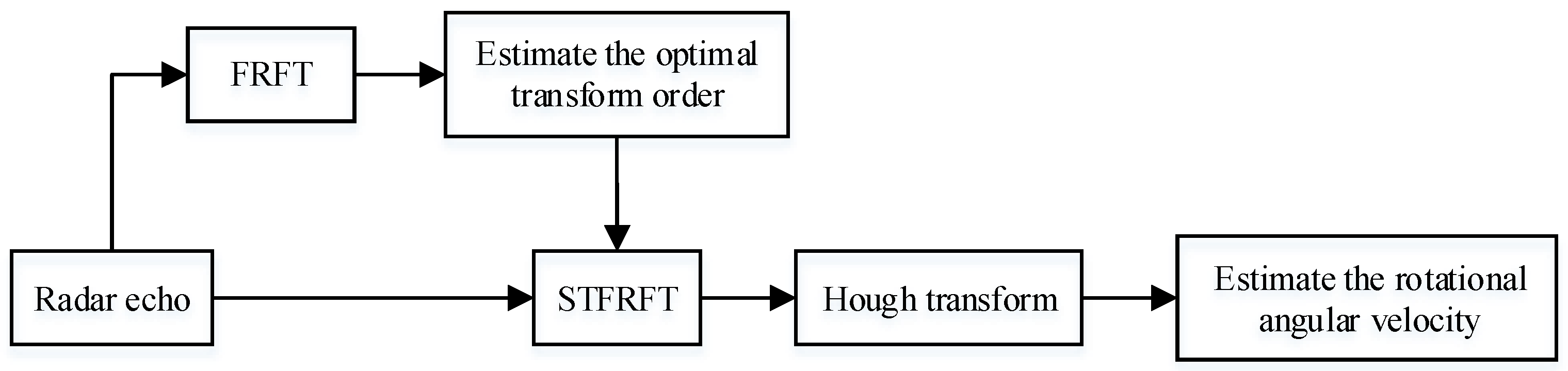
One can see from Equation (10) that the result of STFRFT is not only a time–FRFD–frequency spectrum, but also related to the transform order p, and there is an optimal time-FRFD- frequency spectrum with the highest time–FRFD–frequency resolution in the case of the matched transform order p₀ or the matched transform angle α₀. In practice, the matched transform order p₀, which is an unknown variable, should be estimated from the FRFT result and used in STFRFT to obtain the optimal time–FRFD–frequency spectrum. As a parameter space transform algorithm, Hough transform can realize the energy accumulation from the time–FRFD–frequency spectrum of the target echo. The rotational angular velocity can be estimated according to the peak value of the energy accumulation. The flowchart of the rotational angular velocity estimation method based on STFRFT and Hough transform is shown in Figure 2.

As we can see from Figure 2, in order to obtain the time–FRFD–frequency spectrum with the highest time–FRFD–frequency resolution and accurately estimate the rotational angular velocity, the transform order p used in STFRFT should be estimated and as close as possible to the matched transform order p₀.

3.1. The Traditional Search Method of Estimating the Matched Transform Order

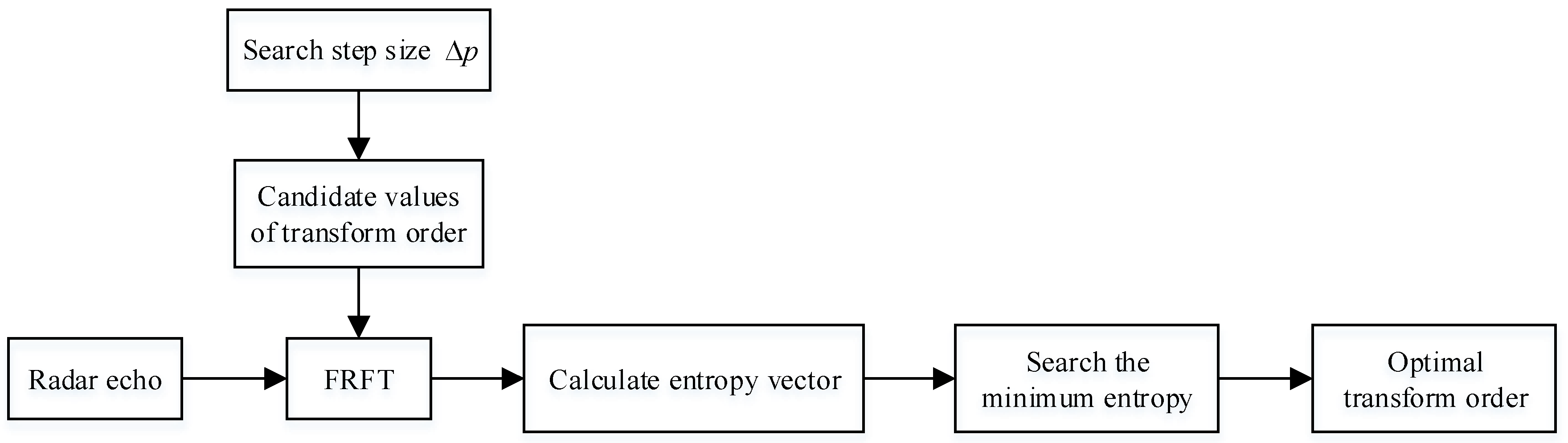
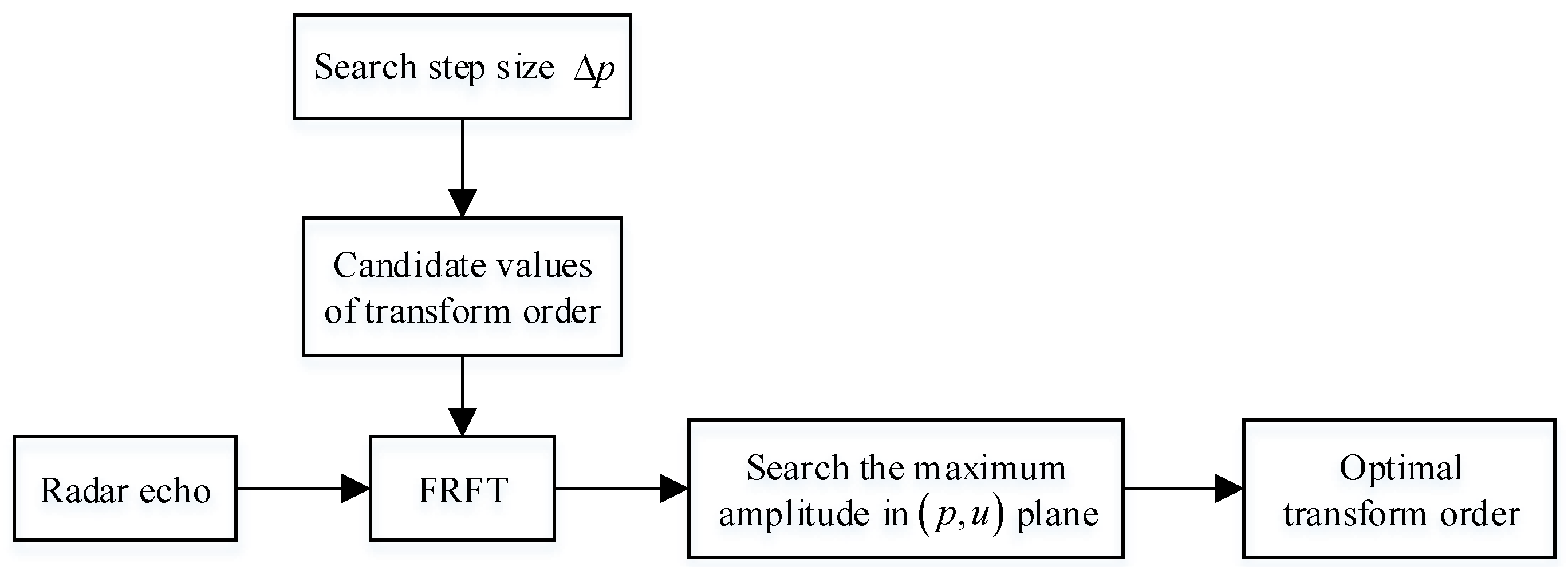
In the traditional search method, the estimation of the matched transform order is to take p as a variable with a search step size of Δp and calculate FRFT of the signal in a two-dimensional energy distribution on the (p,u) plane. All the discretization values of the transform order are regarded as the candidate values. Then we can search the maximum amplitude, which is the highest energy accumulation, and the corresponding transform order candidate is the estimated matched transform order, which we called the optimal transform order. The flowchart of the traditional search method to estimate the matched transform order is shown in Figure 3.

As we can see from Figure 3, each candidate value of the transform order will be used in FRFT. When a candidate value is equal to or close to the matched transform order, the energy of the signal in the FRFT result is the most concentrated. However, there will be a contradiction between the estimation accuracy and the computational complexity in the estimation of optimal transform order ${\widehat{p}}_0$ using the traditional search method. On the one hand, the higher the estimation accuracy, the smaller the search step size of transform order. At the same time, more FRFT times will be implemented, which will lead to greater computational complexity. On the other hand, the computational complexity of the traditional search method can be reduced by increasing the search step size of the transform order or by reducing the number of operations of the FRFT. However, with the increase of the search step size, the estimation accuracy of the optimal transform order will be reduced, resulting in the reduction of the time–FRFD–frequency resolution of the STFRFT, which is not conducive to the estimation of the micro-Doppler parameter of rotational angular velocity. In order to solve this problem, a novel modified short-time fractional Fourier transform algorithm is proposed in this paper, where the problem of searching the maximum amplitude or the maximum energy accumulation in FRFT is converted into the entropy minimization problem and an OMP-based algorithm is proposed to reduce the computational complexity in the estimation of the matched transform order.

3.2. The Proposed OMP-Based Algorithm of Estimating the Matched Transform Order

Different transform orders correspond to different maximum amplitude values of FRFT results. When the candidate value of transform order is equal to the matched transform order, the maximum amplitude value of FRFT results reaches the maximum. Although we can estimate the matched transform order by searching the maximum amplitude value of the FRFT result, it is easy to be affected by noise, which leads to inaccurate estimation of the matched transform order. As we all know, entropy can effectively measure the focusing of signal energy [38], and the more concentrated the signal energy is, the smaller the corresponding entropy is. When the candidate value of the transform order is equal to the matched transform order, the energy accumulation in FRFT result is the strongest, and the corresponding entropy is the smallest. Therefore, the matched transform order can be effectively estimated by calculating the entropy of the FRFT result and searching the minimum entropy.

The transform order of FRFT is related to the rotation angle of time–frequency axis, so FRFT has the characteristics of periodicity and symmetry with transform order as an independent variable [39], where the period is 4 and the axis of symmetry within a period [0, 4] is p = 2. Therefore, it only needs to consider the FRFT results with the transform order in the range of [0, 2] in the traditional search method. It is assumed that the variable p is discretized by the search step size Δp in the range of [0, 2] to P = [p₁,…p_i,…,p_N]^T, which we called the candidate values of the transform order. The total number of candidate values is $N=\lfloor 2/\Delta p\rfloor$, where $\lfloor \cdot \rfloor$ represents the rounding down operation. The discrete form of the echo signal s_F(t_m) of the range unit where the target is located can be expressed as:

$$s_F=\left[s_F\left(1\right),s_F\left(2\right),\cdots ,s_F\left(M\right)\right],$$

(12)

where M is the number of echo pulses in one observation time. According to Equation (7), the FRFT result of the echo signal with the candidate value of the transform order p_i is:

$$FRF{T}_{p_i}=\left[{\mathrm{FRFT}}_{p_i}\left(1\right),{\mathrm{FRFT}}_{p_i}\left(2\right),\cdots {\mathrm{FRFT}}_{p_i}\left(M\right)\right].$$

(13)

The entropy of the FRFT result can be calculated as:

$$E_{p_i}=-{\displaystyle \sum _{m=1}^M\left(\frac{{\mathrm{FRFT}}_{p_i}{}^2\left(m\right)}{{\Vert FRF{T}_{p_i}\Vert }_2}\ln \frac{{\mathrm{FRFT}}_{p_i}{}^2\left(m\right)}{{\Vert FRF{T}_{p_i}\Vert }_2}\right)}=-{\displaystyle \sum _{m=1}^M\left(\frac{{\mathrm{FRFT}}_{p_i}{}^2\left(m\right)}{{\displaystyle \sum _{l=1}^M{\mathrm{FRFT}}_{p_i}{}^2\left(l\right)}}\ln \frac{{\mathrm{FRFT}}_{p_i}{}^2\left(m\right)}{{\displaystyle \sum _{l=1}^M{\mathrm{FRFT}}_{p_i}{}^2\left(l\right)}}\right)},$$

(14)

where ${\Vert \cdot \Vert }_2$ represents the 2-norm. All the candidate values of transform order P are used in FRFT and the corresponding complete entropy vector can be expressed as:

$$E={\left[E_{p_1},\cdots E_{p_i},\cdots E_{p_N}\right]}^{\mathrm{T}}.$$

(15)

The minimum entropy value can be found from the entropy vector, and the corresponding candidate value of transform order is the optimal transform order where we call this method the minimum entropy criterion-based optimal transform order estimation method, and the flowchart of this method is summarized and shown in Figure 4.

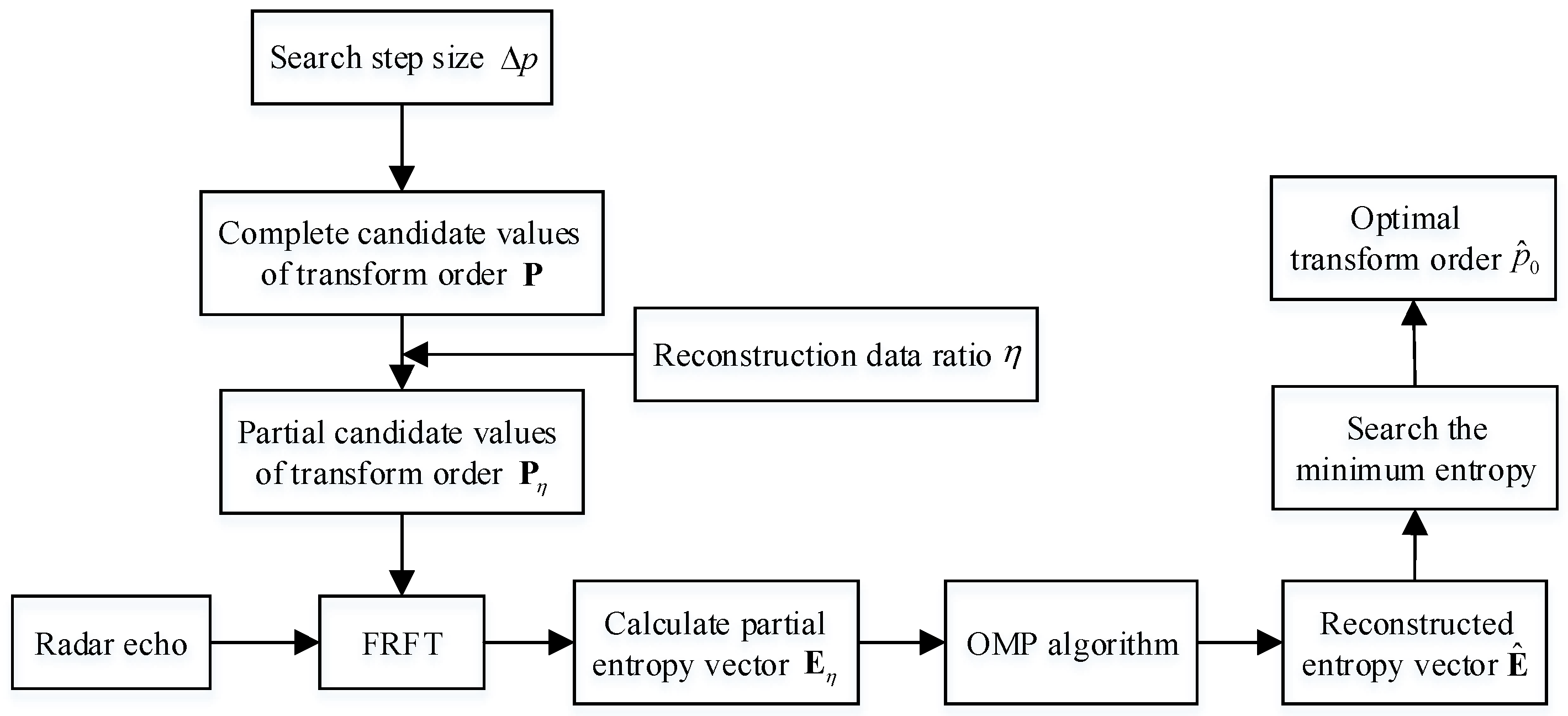
In order to reduce the computational complexity of the optimal transform order estimation in the traditional search method, partial candidate values of the transform order P_η are selected randomly with a ratio η (0 ≤ η ≤ 1), which we called the reconstruction data ratio, from the complete candidate values of the transform order P. Then, a partial entropy vector Eη corresponding to the selected candidate values of the transform order is calculated. Finally, the OMP algorithm is utilized to reconstruct the complete entropy vector E, and the optimal transform order can be estimated by searching the minimum entropy from the reconstructed entropy vector $\widehat{E}$.

Partial candidate values of the transform order P_η can be expressed as:

$$P_{\eta }={\left[p_1,\cdots p_j,\cdots p_{N_{\eta }}\right]}^{\mathrm{T}},$$

(16)

where $N_{\eta }=\lfloor N\cdot \eta \rfloor$ is the total number of the partial candidate values of the transform order and P_η is selected randomly from P, that is, P_η ⊆ P. The random selection process can be described by a matrix multiplication as:

$$P_{\eta }=\Phi \cdot P,$$

(17)

where Φ is a partial unit matrix of size N_η × N, which is called dictionary matrix, and it can be obtained according to the position of the transform order selected from the complete candidate values P in advance. The elements in the dictionary matrix Φ take values from $\left\{0,1\right\}$. Only one element in each row is 1, and the rest are 0. Taking 1 means that the samples at the corresponding position in P are selected in P_η. Each candidate value of P_η is carried into Equations (13) and (14), and the partial entropy vector can be expressed as:

$$E_{\eta }=\Phi \cdot E,$$

(18)

where E_η is a measurement vector of size N_η × 1, and $E\in {ℝ}^{N\times 1}$ is the sparse entropy vector to be reconstructed and solved.

According to the theory of compressed sensing, the OMP-based sparse optimization algorithm can be used to solve Equation (18) to get sparse solution $\widehat{E}$, which can be expressed as:

$$\widehat{E}=\underset{E}{\arg \min }{\Vert E\Vert }_0\hspace{0.17em}\hspace{0.17em}\hspace{0.17em}\hspace{0.17em}\mathrm{s}.\mathrm{t}.\hspace{0.17em}\hspace{0.17em}{E}_{\eta }-\Phi E\le {\epsilon }_0,$$

(19)

where ${\Vert \cdot \Vert }_0$ denotes L₀ norm, and ε₀ denotes the error threshold in the sparse recovery processing. The optimal transform order can be estimated by searching the minimum entropy from the reconstructed entropy vector, which can be expressed as:

$${\widehat{p}}_0=\underset{p_i}{\arg \min }\widehat{E}.$$

(20)

To sum up, the flowchart of the proposed OMP-based algorithm of estimating the matched transform order is summarized in Figure 5, and the main steps of the OMP algorithm to reconstruct the complete entropy vector are shown in Algorithm 1.

Algorithm 1 Main steps of the OMP algorithm to reconstruct the complete entropy vector.

Input: measurement vector $E_{\eta }\in {ℝ}^{N_{\eta }}$, dictionary matrix $\Phi \in {\mathbb{Z}}^{N_{\eta }\times N}$, error threshold ε0.

Initialization: let the iterative counter k = 1, residual matrix γ0 = Eη, the index set ${\Lambda }_0=\mathsf{\varnothing }$.

Iteration: at the k-th iteration

(1) Update the index set ${\Lambda }_k={\Lambda }_{k-1}\cup {\lambda }_k$, where ${\lambda }_k=\underset{i=1,2,\cdots ,N}{\arg \max }\left|\langle {\gamma }_{k-1},{\phi }_i\rangle \right|$, φi is the i-th column of Φ.

(2) Update the support set ${\Phi }_{{\Lambda }_k}=\left[{\Phi }_{{\Lambda }_{k-1}},{\phi }_{{\lambda }_k}\right]$, and calculate the signal ${\widehat{E}}_k=\arg \max {\Vert E_{\eta }-{\Phi }_{{\Lambda }_k}{E}_k\Vert }_2={\left({\Phi }_{{\Lambda }_k}{}^{\mathrm{H}}{\Phi }_{{\Lambda }_k}\right)}^{-1}{\Phi }_{{\Lambda }_k}{}^{\mathrm{H}}{E}_{\eta }$.

(3) Update the residual matrix ${\gamma }_k=E_{\eta }-{\Phi }_{{\Lambda }_k}{\widehat{E}}_k$.

(4) Increment k, and return to Step (1) until the stopping criterion ${\Vert {\gamma }_k\Vert }_2\le {\epsilon }_0$ is met. The selection of the error threshold ε0 is related to the precision requirement.

Output: Reconstructed entropy vector $\widehat{E}={\widehat{E}}_k$.

3.3. Rotational Angular Velocity Estimation via Modified Short-Time Fractional Fourier Transform

In this paper, the estimated matched transform order ${\widehat{p}}_0$ is used in STFRFT to obtain the time–FRFD–frequency spectrum that has the highest time–FRFD–frequency resolution compared to other spectra corresponding to other candidate values of the transform order. After the time FRFD-frequency domain is characterized by the STFRFT, the Hough transform is employed to map the time FRFD-frequency domain on the micro-Doppler parameter space {ω,r,θ}, where ω, r, and θ denote the rotational angular velocity, the length, and initial phase of the rotor blades, respectively. The Hough transform for parameter estimation of sinusoidal frequency modulated signals is defined as:

$$H\left(\omega ,r,\theta \right)={\displaystyle {\int }_{T_a}\left|{\mathrm{STFRFT}}_{{\widehat{p}}_0}\left[t,2\omega r\sin \left(\omega t+\theta \right)/\lambda \right]\right|\mathrm{d}t},$$

(21)

where $|\cdot |$ denotes the absolute value symbol, ${\mathrm{STFRFT}}_{{\widehat{p}}_0}\left[t,2\omega r\sin \left(\omega t+\theta \right)/\lambda \right]$ is the STFRFT result obtained by Equation (10) with the optimal transform order ${\widehat{p}}_0$ and is the time–FRFD–frequency spectrum with the Doppler frequency change rule $f_d=2\omega r\sin \left(\omega t+\theta \right)/\lambda$.

As we can see from Equation (21), the result of the Hough transform is not only related to the length and initial phase of the rotor blades, but also to the rotational angular velocity of the rotor target. We can also say that these three variables determine the trajectory of Hough transform to accumulate energy and should be discretized into multiple candidate values before Hough transform, i.e., ${\omega }_i\in \left\{{\omega }_1,\cdots ,{\omega }_i,\cdots ,{\omega }_{N_{\omega }}\right\}$, $r_i\in \left\{r_1,\cdots ,r_i,\cdots ,r_{N_r}\right\}$ and ${\theta }_i\in \left\{{\theta }_1,\cdots ,{\theta }_i,\cdots ,{\theta }_{N_{\theta }}\right\}$, where N_ω, N_r and N_θ represent the number of discrete values of three variables ω, r, and θ, respectively. For each candidate value of the rotational angular velocity ω_i, there will be an energy accumulation spectrum in the two-dimensional parameter space {r,θ}. When a rotational angular velocity candidate value is equal to or close to the real rotational angular velocity of the rotor target, the energy accumulation spectrum in two-dimensional parameter space {r,θ} has the highest energy accumulation peak. Therefore, we can search the peak value from the energy accumulation spectrum in two-dimensional parameter space {r,θ} to estimate the rotational angular velocity of the rotor target. This estimation process of rotational angular velocity can be expressed as:

$$H_v\left(\omega \right)=\underset{\left\{{\omega }_i,H\left(\omega ,r,\theta \right)\right\}}{\arg \max }H\left(\omega ,r,\theta \right),$$

(22)

$${\widehat{\omega }}_0=\underset{{\omega }_i}{\arg \max }{H}_v\left(\omega \right),$$

(23)

where H_v(ω,v) denotes the peak value of energy accumulation corresponding to different candidate values of the rotational angular velocity, ${\widehat{\omega }}_0$ denotes the estimated rotational angular velocity.

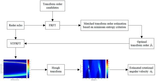
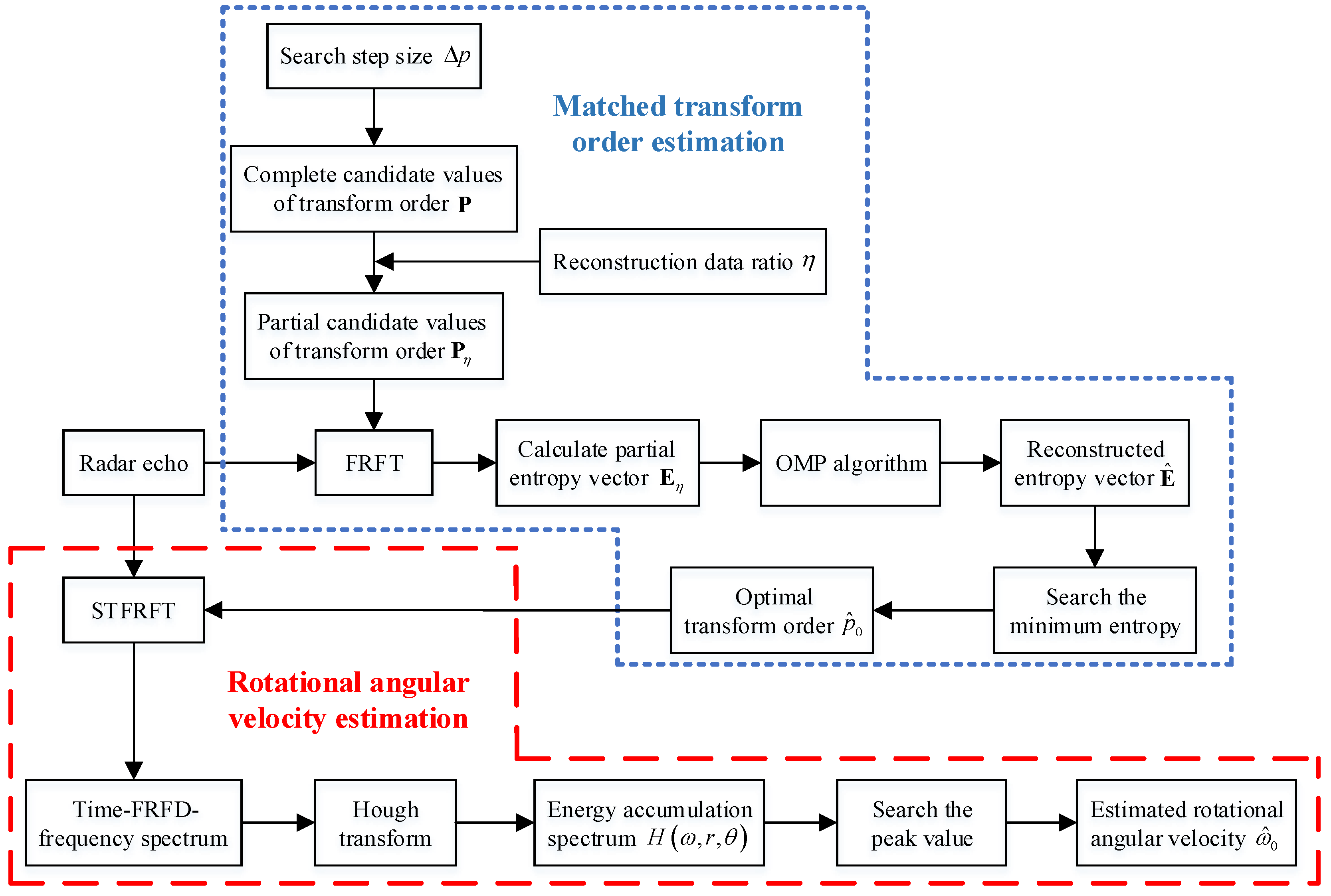
By accurately estimating the optimal transform order, the rotational angular velocity of the rotor target can be estimated by searching the peak value from the energy accumulation spectrum obtained by Hough transform. To summarize, the complete procedure of the proposed method for rotational angular velocity estimation of rotor target is shown in Figure 6, in which the process in the blue dotted box is the matched transform order estimation based on the OMP algorithm and the process in the red dashed box is the rotational angular velocity estimation based on the combination of the M-STFRFT algorithm and Hough transform.

3.4. Computational Complexity Analysis

Compared with the traditional search method where 100% transform order candidates are selected, the proposed sparse-based method only selects partial transform order candidates and realizes the estimation of matched transform order through OMP reconstruction algorithm, so it is computationally efficient, because fractional Fourier transform and entropy operation corresponding to several transform order candidates are avoided. The following is a comparative analysis of the computational complexity between the traditional search method and the proposed sparse-based method, in which we take an addition, multiplication, and logarithm operation as a calculating unit.

In the traditional search method where 100% transform order candidates are selected, the computational complexity depends on the discrete FRFT and entropy operation. The digital computation of FRFT requires only a sequence of FFTs with the computational complexity O(Mlog₂M), the entropy operation of Equation (14) requires the computational complexity of O(4M). Therefore, the total computational complexity of the traditional search method where 100% transform order candidates are selected can be expressed as:

$$C_{search-method}=O\left(MN{\log }_{2}M+4MN\right).$$

(24)

Suppose that the data ratio of selected transform order candidates is η in the proposed sparse-based method. The computational complexity of the OMP reconstruction algorithm is O(N_ηN). The whole process of the proposed sparse-based method consists of N_η FRFTs, N_η entropy operations, and one OMP reconstruction operation, so the total computational complexity can be given by:

$$C_{proposed-method}=O\left(M{N}_{\eta }{\log }_{2}M+4M{N}_{\eta }+N_{\eta }N\right).$$

(25)

As we can see from Equations (24) and (25), the computational complexity of the traditional search method and the proposed sparse-based method are related to the search step size Δp and reconstruction data ratio η. The comparison between Equations (24) and (25) implies that the computational complexity of the proposed sparse-based method is much less than that of the traditional search method where 100% transform order candidates are selected, which will be validated through the simulation of computation time in Section 4.3.

4. Experimental Results

In this section, several comparative experiments of simulated data are conducted, and simulation results based on measured data collected by frequency modulated continuous wave radar are presented to validate the performance and effectiveness of the proposed algorithm. We consider that a monostatic early warning radar and the micro-Doppler signals are simulated by rotation of the rotor blades in a helicopter, the main rotor part consists of two blades, and the blade length is 6 m. Suppose that there is a scatterer at the outermost end of each blade, so the echo signal contains two micro-Doppler components that we call rotor echo with the same rotational angular velocity and different initial phases. In this experiment, the main parameters of the transmitted signal and the rotor part are summarized in

Table 1. Main parameters of the transmitted signal and the rotor part.

Transmitted signal parameters	Carrier frequency	Bandwidth	Pulse repetition frequency	Observation time	Pulse samples
Value	1 GHz	2 MHz	5 kHz	25 ms	125
Rotor part parameters	Blade number	Blade length	Rotational angular velocity	Initial phase 1	Initial phase 2
Value	2	6 m	25 rad/s	π/2	3π/2

.

The simulation experiments are composed of five parts: (1) simulations to analyze the influence of the transform order on parameter estimation; (2) simulations to select the parameters of the OMP reconstruction algorithm in the estimation of matched transform order; (3) simulations to validate the effectiveness of the proposed algorithm; (4) comparative experiments of parameter estimation among time–frequency analysis algorithms; (5) verification experiment based on measured data.

4.1. Influence Analysis of the Transform Order on Parameter Estimation

In the experiment, we consider the noise-free case and investigate the influence of the transform order used in STFRFT on the estimation of the rotational angular velocity. The rotating part consists of two blades with the same rotational angular velocity ω = 25 rad/s and different initial phase π/2 and 3π/2. Therefore, two different micro-Doppler components caused by them in the echo signal have different chirp rates, corresponding to different matched transform orders. 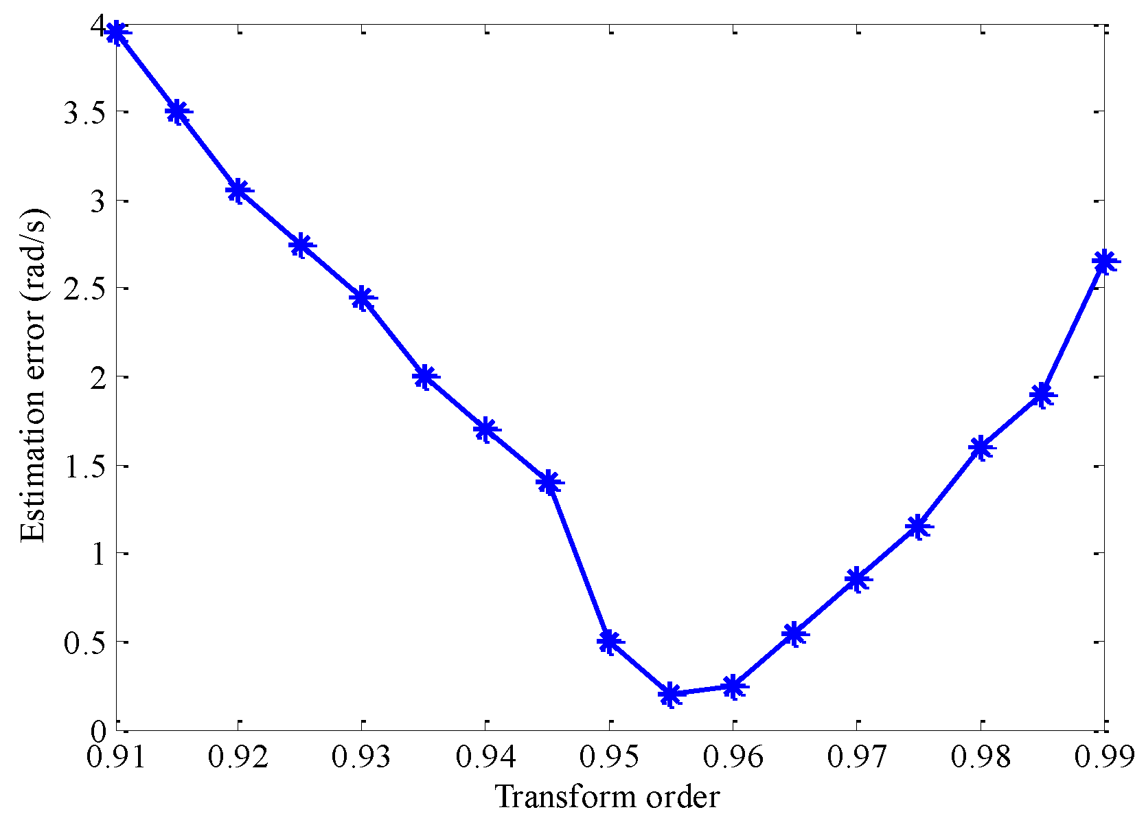According to the parameters of radar transmitting signal and Equation (9), we can calculate that the matched transform orders of echo components with initial phases of π/2 and 3π/2 are p₀₁ = 0.9535 and p₀₂ = 1.0465, respectively. We take the transform order as a variable, which is ranged from 0.91 to 0.99 with a step size of 0.05, and each transform order is used as the optimal transform order in STFRFT. Therefore, multiple time–FRFD–frequency spectra corresponding to different transform orders can be obtained, and then the rotational angular velocity of the rotor target can be estimated by Hough transform and energy peak search. The simulation result of the estimation error of rotational angular velocity is shown in Figure 7, from which one can see that the estimation error of rotational angular velocity is the smallest when the transform order is 0.955, which is close to the matched transform order p₀₁. We can also see that the farther the transform order is away from the matched transform order, the greater the estimation error of the rotational angular velocity is. Therefore, it can be concluded that: (1) the matched transform order is the optimal transform order because of the smallest estimation error of the rotational angular velocity; (2) when STFRFT is used in parameter estimation, it is not only necessary to estimate the matched transform order to improve the estimation accuracy of the rotational angular velocity but also to reduce the computational complexity of the algorithm, that is, to solve the contradiction between the estimation accuracy and the calculation speed.

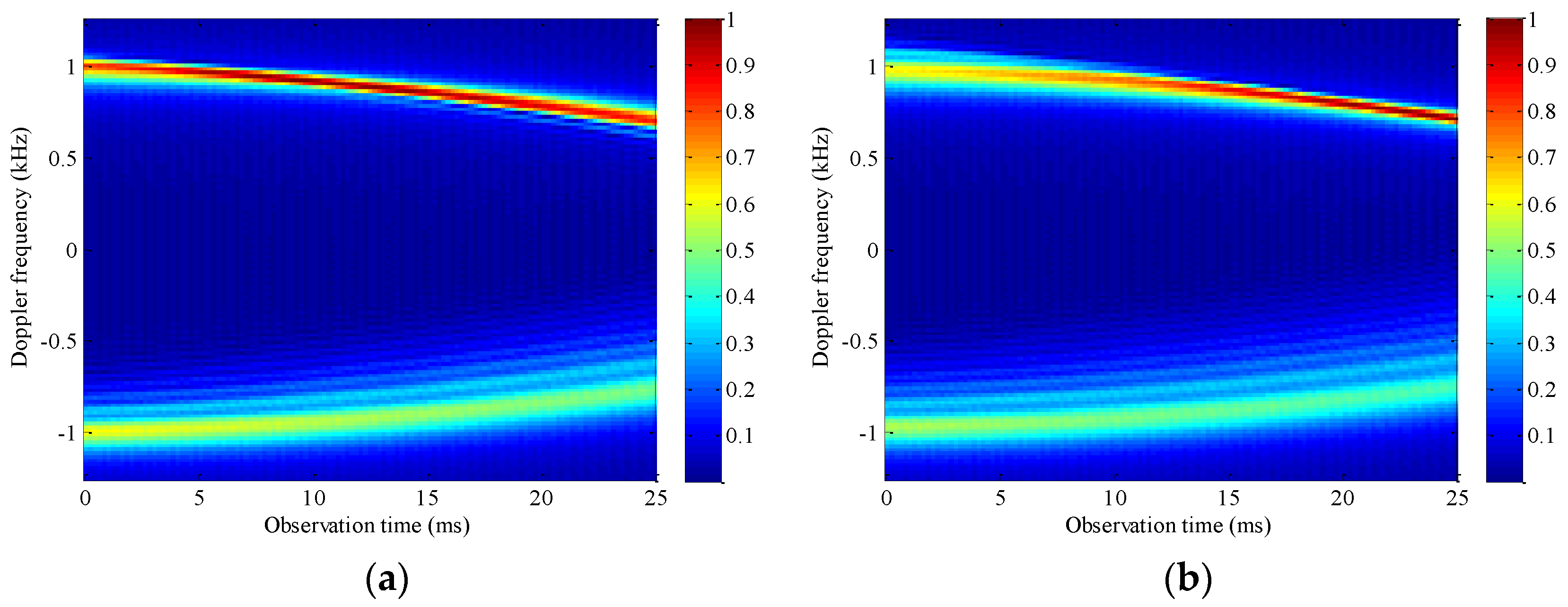
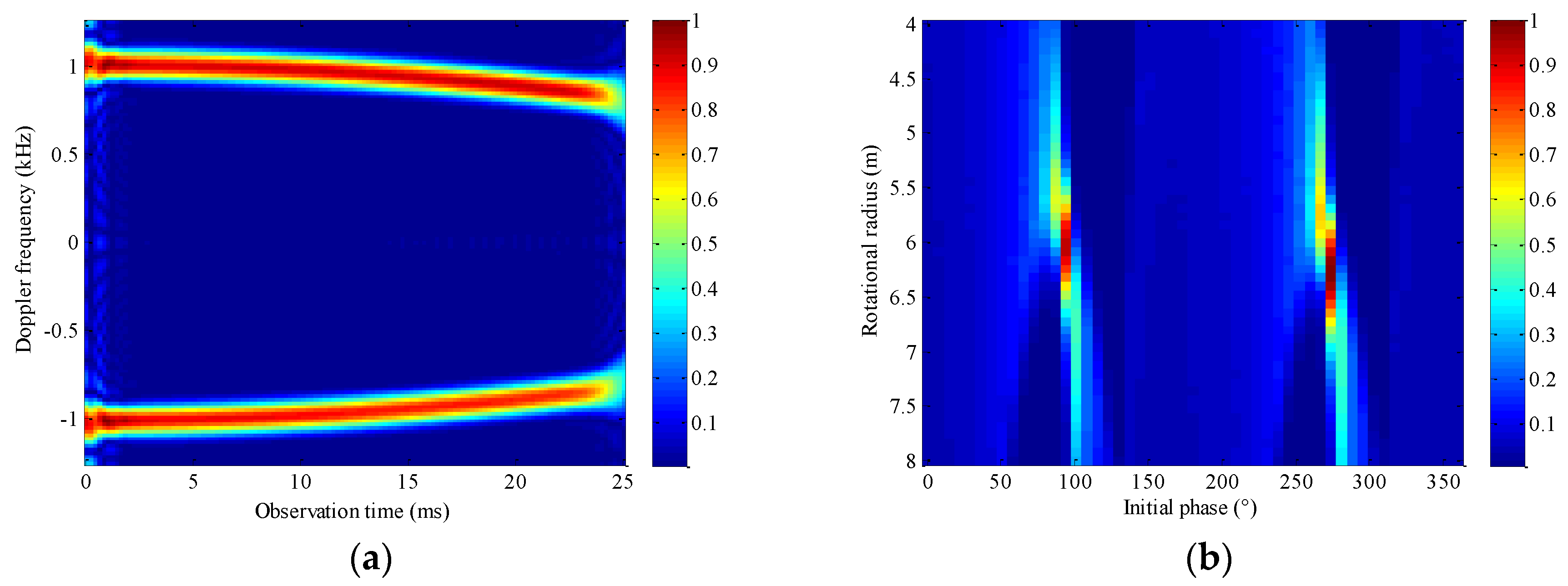
Figure 8 shows the results of the time–FRFD–frequency spectrum of target echo signal under different transform orders. For the echo signal with multiple micro-Doppler components, each matched transform order can only ensure that the time–FRFD–frequency spectrum of the corresponding echo component has a higher time–FRFD–frequency resolution, while the other echo components cannot be effectively accumulated due to the mismatch of the rotation angle. Figure 8a is the result of STFRFT with the transform order of 0.955, since the transform order 0.955 is closer to the matched transform order of the echo component with the initial phase π/2, the time–FRFD–frequency resolution of this component is higher, while that of the echo component with initial phase 3π/2 is lower. However, this result does not degrade the estimation accuracy of the rotational angular velocity, because these echo components are from different blades of the same rotating part with the same rotational angular velocity. As long as one echo component has the highest time–FRFD–frequency resolution, it can accurately estimate the rotational angular velocity through the signal energy peak accumulated by the Hough transform. In Figure 7, the estimation error of the rotational angular velocity is the smallest with the transform order of 0.955, which can also be confirmed from Figure 8a. Compared with the time–FRFD–frequency spectrum with the transform order of 0.91 in Figure 8b, the closer the transform order is to the matched transform order, the higher the time–FRFD–frequency resolution, and the more concentrated the echo signal energy accumulated by the Hough transform.

4.2. Parameters Selection of OMP Reconstruction Algorithm in the Estimation of Matched Transform Order

In order to solve the contradiction between the estimation accuracy and the computational complexity, an OMP-based matched transform order estimation algorithm is presented in the proposed M-STFRFT algorithm, in which transform order candidate values with a certain ratio are randomly selected from the search range from 0 to 2, and the entropy value of each searched transform order’s FRFT result is calculated. Then, based on the compression sensing theory, the OMP algorithm is used to reconstruct the complete entropy vector, and the matched transform order is estimated according to the position of the minimum entropy. There is no doubt that the reconstruction data radio and the search step size of the transform order are the key factors that directly affect the estimation accuracy and the computational complexity.

In this experiment, we first investigate the influence of the reconstruction data ratio of transform order on the estimation accuracy of the rotational angular velocity in a noise environment. It is assumed that the search step size of the transform order is a constant value of 0.001, and the received signal is added with white Gaussian noise and the signal-to-noise (SNR) is defined as $\mathrm{SNR}={\Vert s_r\left(\widehat{t},t_m\right)\Vert }_2^2/\left(M{\sigma }_0{}^2\right)$, where $s_r\left(\widehat{t},t_m\right)$ is the echo signal without pulse compression in Equation (3) and ${\sigma }_0{}^2$ is the variance of the noise. 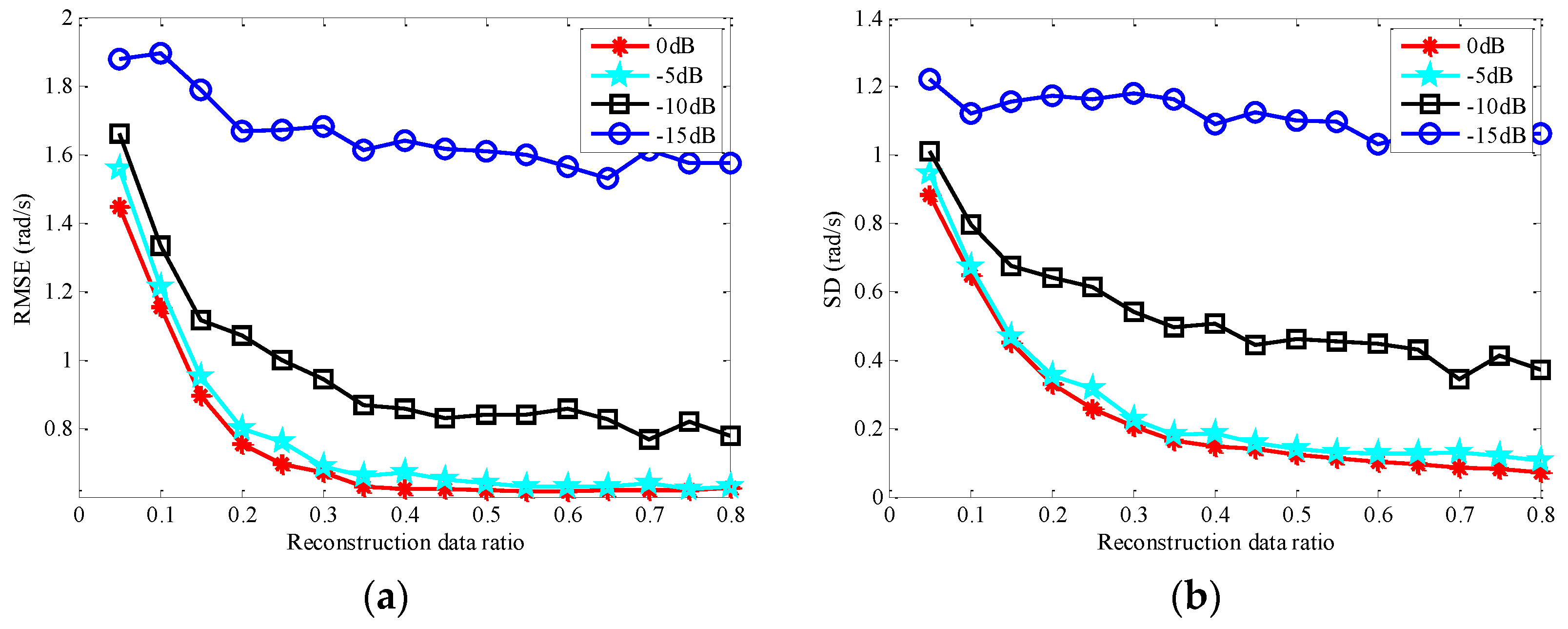Figure 9 plots the estimation error, such as root-mean-square error (RMSE) and standard deviation (SD), of rotational angular velocity varying different reconstruction data ratio of the transform order. The calculation formulas of RMSE and SD are $\mathrm{RMSE}=\sqrt{{\displaystyle \sum _{n=1}^N{\left({\widehat{\omega }}_n-\omega \right)}^2}/N}$ and $\mathrm{SD}=\sqrt{{\displaystyle \sum _{n=1}^N{\left({\widehat{\omega }}_n-\overline{\omega }\right)}^2}/N}$, where ${\widehat{\omega }}_n$, $\overline{\omega }$, and ω denote estimated value, mean of the estimated value, and true value of the rotational angular velocity, respectively. N = 1000 is the number of estimated values, that is, each value of RMSE and SD is obtained and averaged by 1000 Monte-Carlo trials.

As we can see from Figure 9, on the one hand, with the increase of reconstruction data ratio of transform order from 0.05 to 0.8, the estimated RMSE and SD of rotational angular velocity decrease gradually under the same SNR. We can also see that the smaller the reconstruction data ratio, the larger the estimation error of rotational angular velocity, the more unstable the estimation, and the greater the change of estimated RMSE and SD. In addition, when the reconstruction data ratio of transform order exceeds 0.5, the change of estimated RMSE and SD is very small. On the other hand, under the same reconstruction data ratio of transform order, the lower the SNR of the target echo, the greater the change of the estimated RMSE and SD. Moreover, one can see that the estimated RMSE and SD of the rotational angular velocity with the contrastive SNR of 0 dB and −5 dB are similar. However, for the same SNR variation of 5 dB, the estimated RMSE and SD corresponding to the SNR of −10 dB and −15 dB change greatly, which shows that the effect of the SNR on estimated RMSE and SD of rotational angular velocity changes nonlinearly.

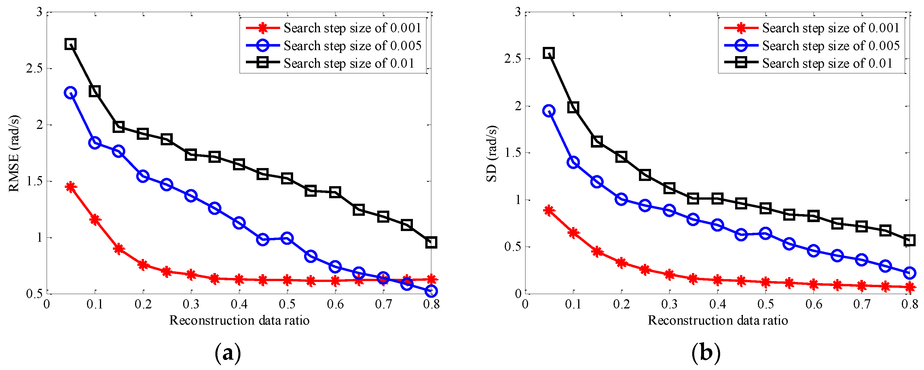
In order to investigate the influence of both the search step size and reconstruction data radio of the transform order on the estimation of rotational angular velocity, we do this experiment in a noise environment with an SNR of 0 dB. The results of the estimated RMSE and SD of the rotational angular velocity are shown in Figure 10, which varies both reconstruction data ratio and search step size of the transform order. As we can see from Figure 10, with the increase of the reconstruction data ratio of transform order, the estimated RMSE and SD of rotational angular velocity decrease gradually and change more slowly under the same search step size of transform order. When a lower reconstruction data ratio is adopted to estimate the optimal transform order, there will be a larger deviation between the estimated optimal transform order and the real matched transform order, and a larger estimation error of rotational angular velocity. Additionally, it is easily found that when the search step size of transform order is 0.001, the trend and value of the estimation error of rotational angular velocity in Figure 10 are the same as that in Figure 9. Moreover, with the same reconstruction data ratio, the larger search step size of the transform order can lead to the larger estimation error of the rotational angular velocity. It can be concluded from this experiment that (1) the larger the reconstruction data ratio and the smaller the search step size of the transform order, the more accurate and stable the estimation of the rotational angular velocity, but it will lead to a large amount of computational complexity. (2) When the reconstruction data ratio and the search step size of transform order are 0.5 and 0.001, respectively, the estimated RMSE and SD are not only small but also stable, which shows that the rotational angular velocity estimation is more efficient under this parameters selection.

4.3. Effectiveness Validation of the Proposed Algorithm

In this experiment, two aspects of comparative simulation experiments are implemented to verify the effectiveness of the proposed OMP-based algorithm in estimating the matched transform order. They are the computation time of the algorithm and the estimation error of rotational angular velocity. Firstly, we consider the noise-free case and compare the computation time between the proposed OMP-based method and the traditional search method in the estimation of the matched transform order. The experiments are implemented by using MATLAB 2014a on a PC (Intel Celeron CPU 1007U 1.5 GHz and a 4096-MB memory capacity), and results are shown in Figure 11. 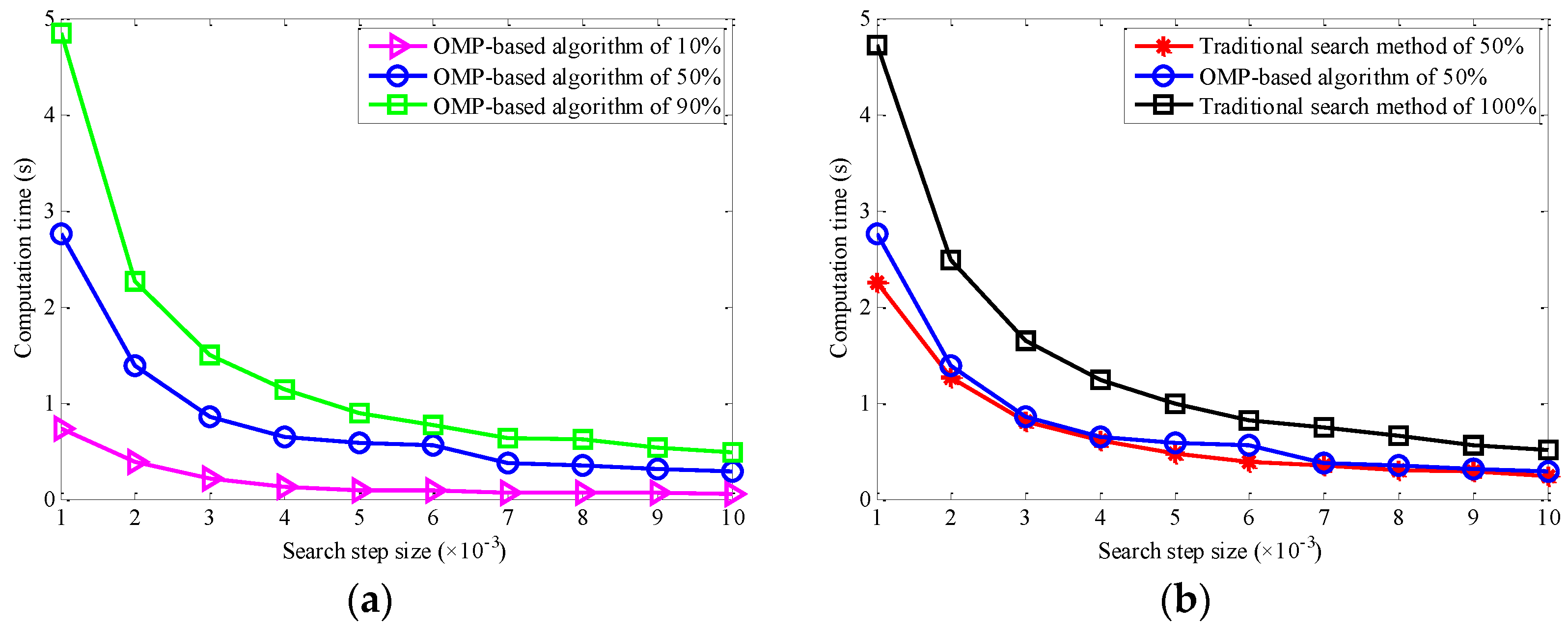Figure 11a plots the comparison of the computation time among the proposed OMP-based algorithm with different reconstruction data ratios of 10%, 50%, and 90%, and Figure 11b plots the comparison of the computation time between the proposed OMP-based algorithm and the traditional search method. It should be pointed out that the difference among the comparative experiments in Figure 11b is the solution of the matched transform order, which can be described as follows: (1) the proposed OMP-based algorithm with the reconstruction data ratio of 50% is utilized to estimate the matched transform order; (2) 50% of transform order candidate values are selected randomly and used to search for the matched transform order in the traditional search method; (3) 100% of transform order candidate values are used for estimating the matched transform order in the traditional search method.

As we can see from Figure 11a, different reconstruction data ratios of 10%, 50%, and 90% are adopted in the proposed OMP-based algorithm in estimating the matched transform order, and the computation time varies with the different reconstruction data ratios and search step sizes. For the same reconstruction data ratio, with the increase of the search step size, the computation time decreases gradually, because the increase of the search step size leads to the decrease of the number of the transform order candidates. We can also see that for the same search step size, the larger the reconstruction data ratio of the selected transform order candidate values, the more FRFT times need to be calculated, so the computation time will be increased. From Figure 11b, we can see that in accordance with the OMP-based algorithm proposed in this paper, no matter whether 50% or 100% of the transform order candidate values are selected in the traditional search method, with the increase of the search step size, the computation time is also gradually reduced. Moreover, under the same search step size, the computation time of the proposed OMP-based algorithm with the reconstruction data ratio of 50% is slightly higher than that of the traditional search method where 50% transform order candidate values are selected, but it is significantly lower than that of the traditional search method where 100% transform order candidate values are utilized, which shows that in order to reduce the computational complexity or computation time in estimating the matched transform order, the OMP-based algorithm proposed in this paper is effective to estimate the matched transform order.

Secondly, we compare the estimation error of the rotational angular velocity between the proposed OMP-based algorithm and the traditional search method. In this comparative experiment, the candidate values of the transform order are from 0 to 2 with a step size of 0.001, and the three estimation methods are the same as mentioned in Figure 11b and are implemented to estimate the matched transform order. Then, the estimated matched transform orders obtained from the above three methods are used in the STFRFT algorithm for obtaining the time–FRFD–frequency spectrum, and the Hough transform is adopted to estimate the rotational angular velocity. 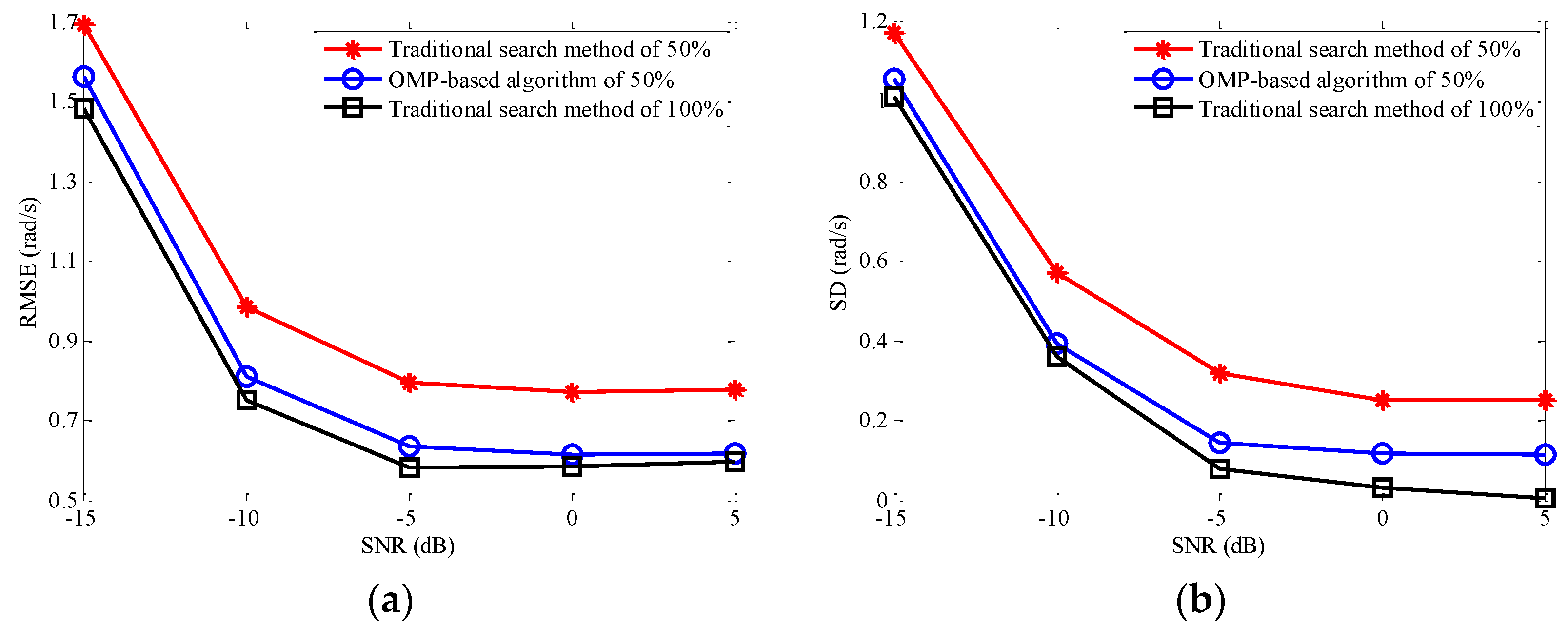The results of the estimation error of rotational angular velocity are shown in Figure 12.

As we can see from Figure 12, with the increase of SNR, the estimation error of rotational angular velocity obtained by any method mentioned above decreases. The reason is that the higher the SNR, the higher the estimation accuracy of the matched transform order whether 50% or 100% of the candidate values are selected in the traditional search method. We can also conclude from Figure 12 that the higher the SNR is, the slower the change of estimation error of RMSE or SD is. Compared with the traditional search method where 100% transform order candidate values are utilized, the traditional search method where 50% transform order candidate values are selected reduces the computational complexity or the computation time displayed in Figure 11b by reducing the number of solutions of optimal transform order. It is actually a kind of increasing the search step size of transform order candidate values in a disguised way, which will lead to the increase of the estimation error between the estimated optimal transform order and the real matched transform order. Then, the resolution of the time–FRFD–frequency spectrum and the estimation accuracy of rotational angular velocity are both reduced, which are confirmed in the results of Figure 12.

Although the OMP-based algorithm proposed in this paper only uses 50% of the transform order candidate values to estimate the optimal transform order in this experiment, it is different from the traditional search method for which 50% transform order candidate values are selected. This proposed OMP-based algorithm combines the compressed sensing theory and estimates the optimal transform order through the OMP reconstruction algorithm, which not only reduces the computational complexity of the algorithm but also can get the optimal transform order more accurately than the traditional search method for which 50% transform order candidate values are selected. It can be seen from Figure 12 that the estimation error of the rotational angular velocity obtained by the proposed OMP-based algorithm in this paper is significantly lower than that of the traditional search method where 50% transform order candidate values are selected but slightly higher than that of the traditional search method with 100% of transform order candidate values are utilized to estimate the optimal transform order. The reason why the estimation accuracy of the rotational angular velocity of the proposed OMP-based algorithm is not up to that of the traditional search method where 100% transform order candidate values are utilized lies in the existence of reconstruction error. It can be concluded from the experimental results that the OMP-based algorithm proposed in this paper is better than the traditional search method using the same data ratio of transform order candidate values in estimating the rotational angular velocity, which indicates that the proposed algorithm can estimate the rotational angular velocity quickly and effectively while ensuring the estimation accuracy.

4.4. Comparative Experiments of Parameter Estimation among Time-Frequency Analysis Algorithms

In this experiment, we first consider the noise-free case and compare the results obtained by the Hough–STFT, the Hough–WVD, the Hough–PWVD, the Hough–RSPWVD, and the proposed algorithm, and then evaluate the estimation error of rotational angular velocity among the aforementioned algorithms in a noise environment. It is assumed that there are two scatterers at the end of the rotor blade on a rotor target with the rotational angular velocity ω = 25 rad/s and the initial phases of each blade at the beginning of the observation are π/2 and 3π/2, respectively, and the blade length is 6 m. Additionally, it is assumed that the translational compensation is carried out to the target echo, so it can be calculated that the maximal Doppler frequency of each rotor echo is 1000 Hz. In the proposed algorithm, the candidate values of the transform order are from 0 to 2 with a search step size of 0.001, and the reconstruction data ratio is set as 50%.

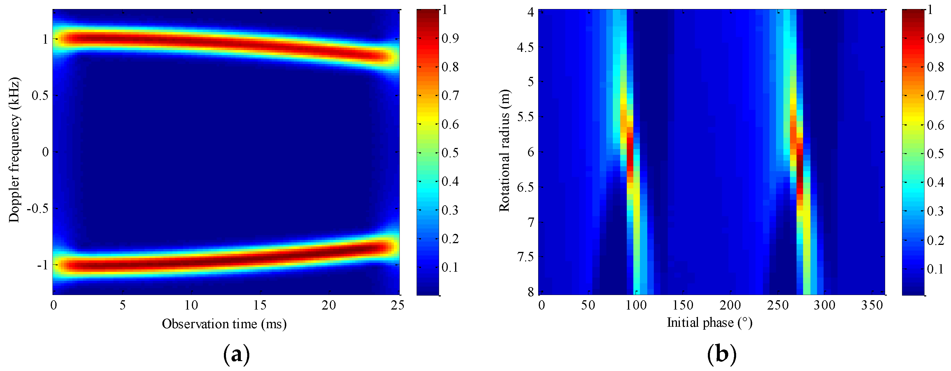
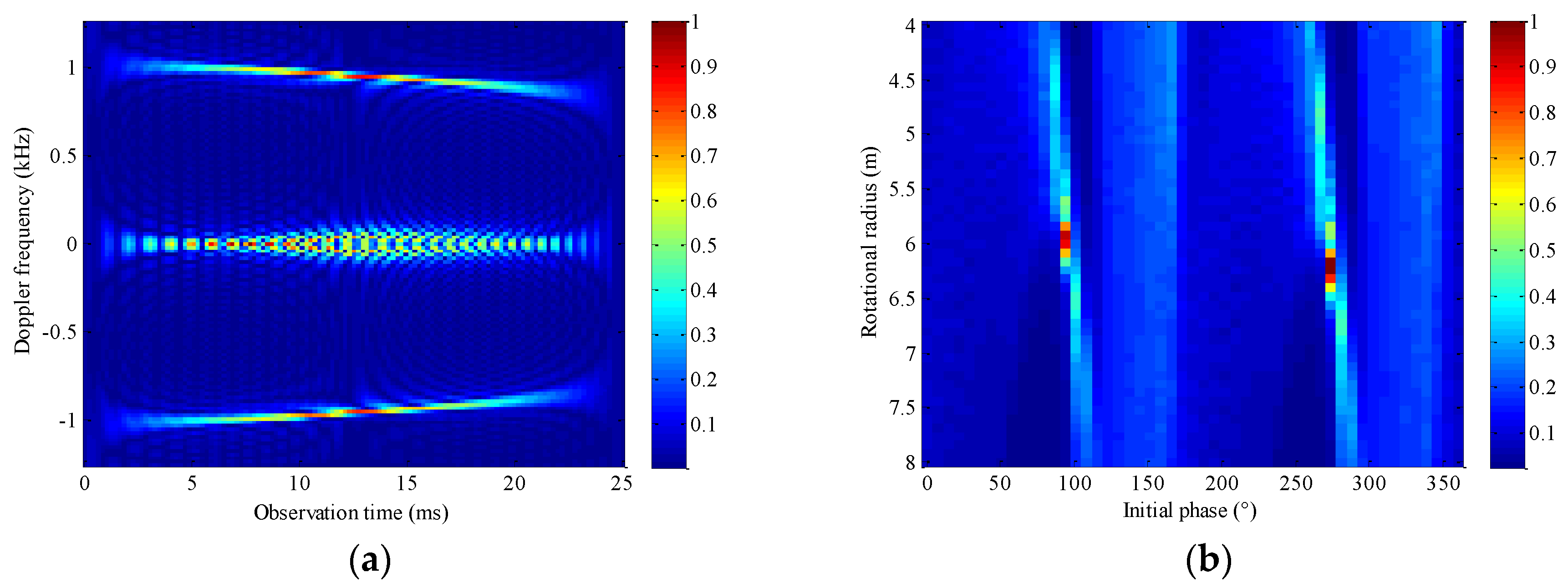
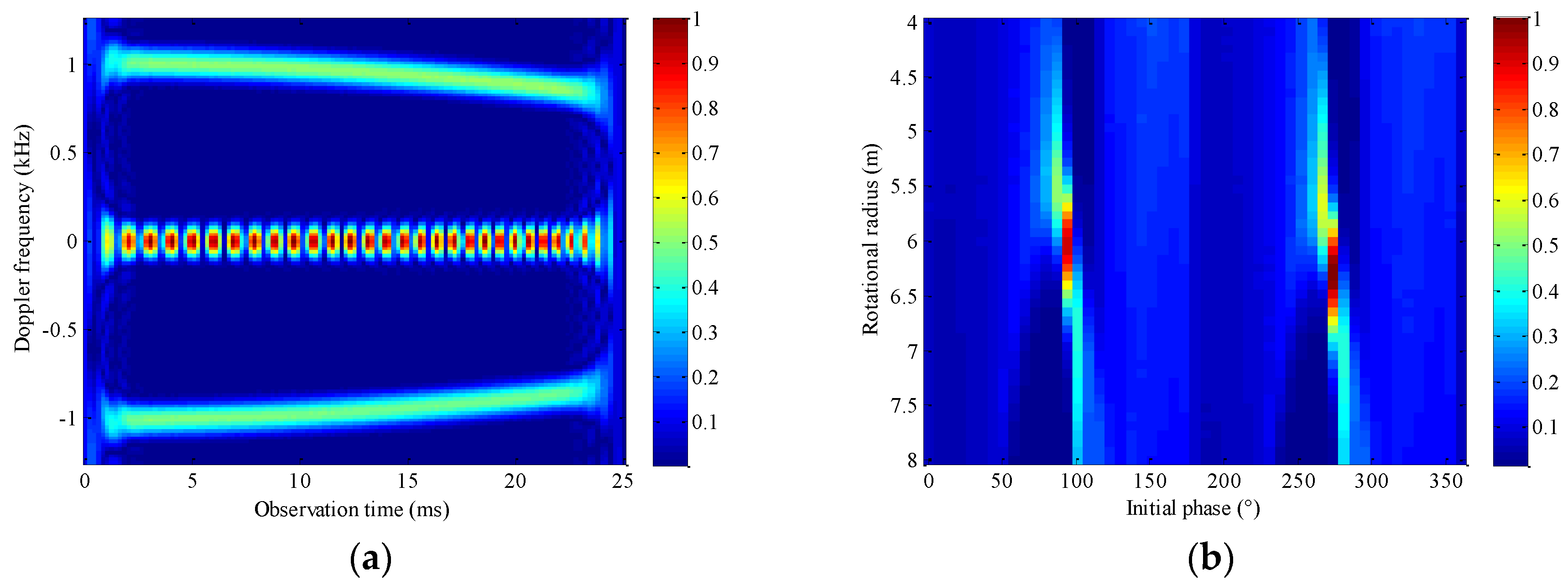
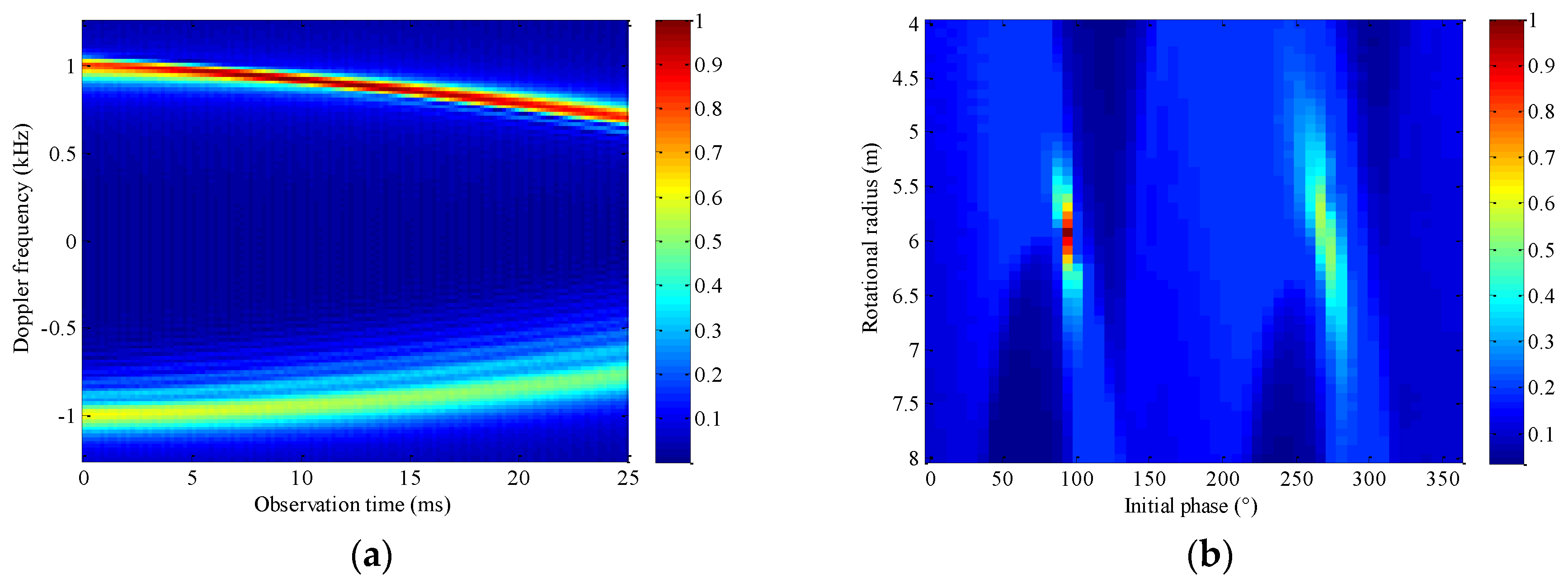
The results obtained by the Hough–STFT, the Hough–WVD, the Hough–PWVD, the Hough–RSPWVD, and the proposed algorithm are provided in Figure 13, Figure 14, Figure 15, Figure 16 and Figure 17, respectively. Figure 13a, Figure 14a, Figure 15a, Figure 16a and Figure 17a show the time–frequency characteristics of the received rotor echo obtained by the STFT, WVD, PWVD, RSPWVD, and the proposed M-STFRFT algorithm, respectively, where the two micro-Doppler components can be seen clearly and the maximal micro-Doppler frequency of each micro-Doppler components is close to the theoretical value 1000Hz. However, as we can see from the figures, STFT and WVD have the problems of low time–frequency resolution and cross-term interference, respectively. To some extent, PWVD and RSPWVD reduce the cross-term interference, but at the same time, the time–frequency resolution is reduced, which is not conducive to the estimation of micro-Doppler parameters. As we can see from Figure 17a, although the resolution of the time–frequency characteristics of a micro-Doppler component is low due to the mismatch with the estimated optimal transform order, the time–FRFD–frequency resolution of another micro-Doppler component corresponding to the estimated optimal transform order is higher than the STFT, PWVD, and RSPWVD algorithm, and there is no cross-term interference in the result obtained by the proposed M-STFRFT algorithm. Therefore, we can estimate the rotational angular velocity effectively by using the high-resolution micro-Doppler component. Compared with the Hough accumulation results in Figure 13b, Figure 14b, Figure 15b and Figure 16b, which display the energy distribution in parameter space {r,θ} and are obtained by Hough transform, the energy of the micro-Doppler component with the highest time–frequency resolution of the proposed algorithm in Figure 17b is more concentrated in the coordinate of the correct value of {r,θ}. Although the energy concentration of the micro-Doppler component with low time–frequency resolution is relatively low, this does not affect the estimation performance of the rotational angular velocity. According to the above simulation results, it can be concluded that the aforementioned time–frequency algorithms are effective for the micro-Doppler parameter of rotational angular velocity estimation and the proposed M-STFRFT algorithm performs more efficiently than the other four algorithms.

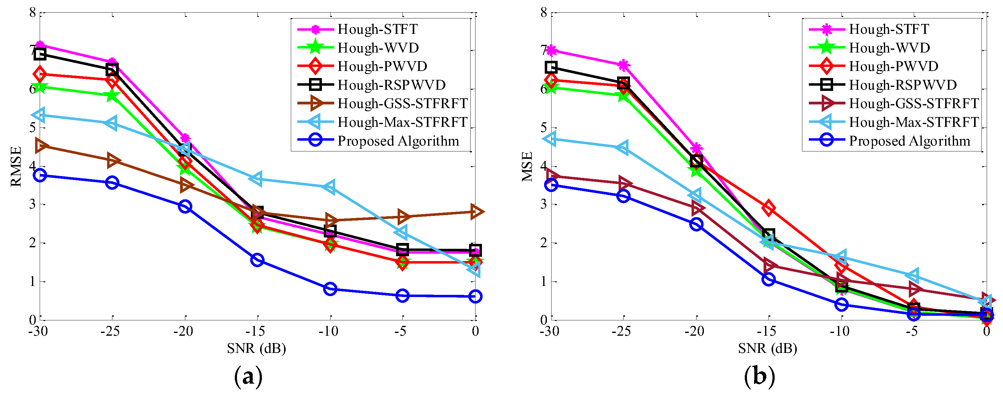
Figure 18 shows the estimated RMSE and SD of rotational angular velocity among the proposed algorithm, the Hough–GSS-based STFRFT algorithm, and other time–frequency analysis algorithms, where the received signal is added with white Gaussian noise, and each value of RMSE and SD are obtained and averaged by 1000 Monte-Carlo trails. It should be pointed out that the rotational angular velocity estimation process of the Hough–GSS-based STFRFT algorithm is the same as that of the algorithm proposed in this paper, except that the Hough–GSS-based STFRFT algorithm adopts the GSS-based FRFT method proposed in [35] when estimating the matched transform order. As a comparison, we give the rotational angular velocity estimation results of the method described in Section 3.1, in which the matched transform order is estimated by searching the maximum amplitude value of FRFT in the traditional method, which is labeled as Hough–Max-STFRFT in Figure 18.

As we can see from Figure 18a,b that with the increase of SNR, the accuracy and stability of the aforementioned estimation algorithms and the proposed algorithm are improved, and finally tend to be stable. We can also see that the Hough–WVD algorithm is more accurate in rotational angular velocity estimation than Hough–STFT, Hough–PWVD, and Hough–RSPWVD algorithms because of the higher time–frequency resolution, while the Hough–STFT algorithm is the least. However, there exists cross-term interference in the WVD algorithm, and the resolution of the WVD algorithm is obviously reduced at the beginning and ending of the observation time, which will lead to the incorrect estimation of the rotational angular velocity and will increase the estimation error of RMSE and SD. By comparing and observing the results of Hough–Max-STFRFT method, we find that the matched transform order estimation method of searching the maximum of FRFT results is easily affected by noise, which leads to inaccurate and unstable estimation of matched transformation order and is not conducive to the estimation of rotational angular velocity. Compared with other time–frequency analysis algorithms, the Hough–GSS-based STFRFT algorithm has a smaller and more stable estimation error under the condition of a low SNR, but it is larger when the SNR is high. Moreover, the estimated RMSE and SD of the Hough–GSS-based STFRFT algorithm in the range of SNR from −30 dB to 0 dB are significantly larger than those of the proposed algorithm. The main reason for this result is that the GSS-based matched transform order estimation algorithm used in the Hough–GSS-based STFRFT algorithm has a local iterative convergence problem.

In the algorithm proposed in this paper, although one micro-Doppler component does not match the estimated optimal transform order, another micro-Doppler component matching the optimal transform order has the highest time–FRFD–frequency resolution, and there is no cross-term interference. Therefore, the proposed algorithm has a higher estimation accuracy of rotational angular velocity than other aforementioned algorithms, which can be reflected in Figure 18a. We can also see that compared with the Hough–GSS-based STFRFT algorithm and other time–frequency analysis algorithms mentioned in this paper, the algorithm proposed in this paper also has better rotational angular velocity estimation performance in the case of low SNR. In summary, we can conclude that the proposed modified short-time fractional Fourier transform has a good performance on rotational angular velocity estimation, which can verify the effectiveness and stability of the algorithm proposed in this paper.

4.5. Verification Experiment based on Measured Data

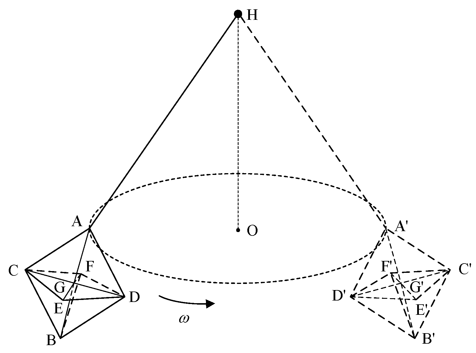
We now present the experimental results based on measured data collected by frequency modulated continuous wave radar, where the carrier frequency is 24 GHz and the pulse repetition interval is 600 μs. The experimental target is a corner reflector with the circular motion. The schematic diagram of experimental scene is shown in Figure 19, where ABCDEF denotes the corner reflector with a circular motion around point O under the action of human factors and traction rope AH, and it moves to A′B′C′D′E′F′ after half a cycle; G is the center of the scatterer; ω denotes the rotational angular velocity.

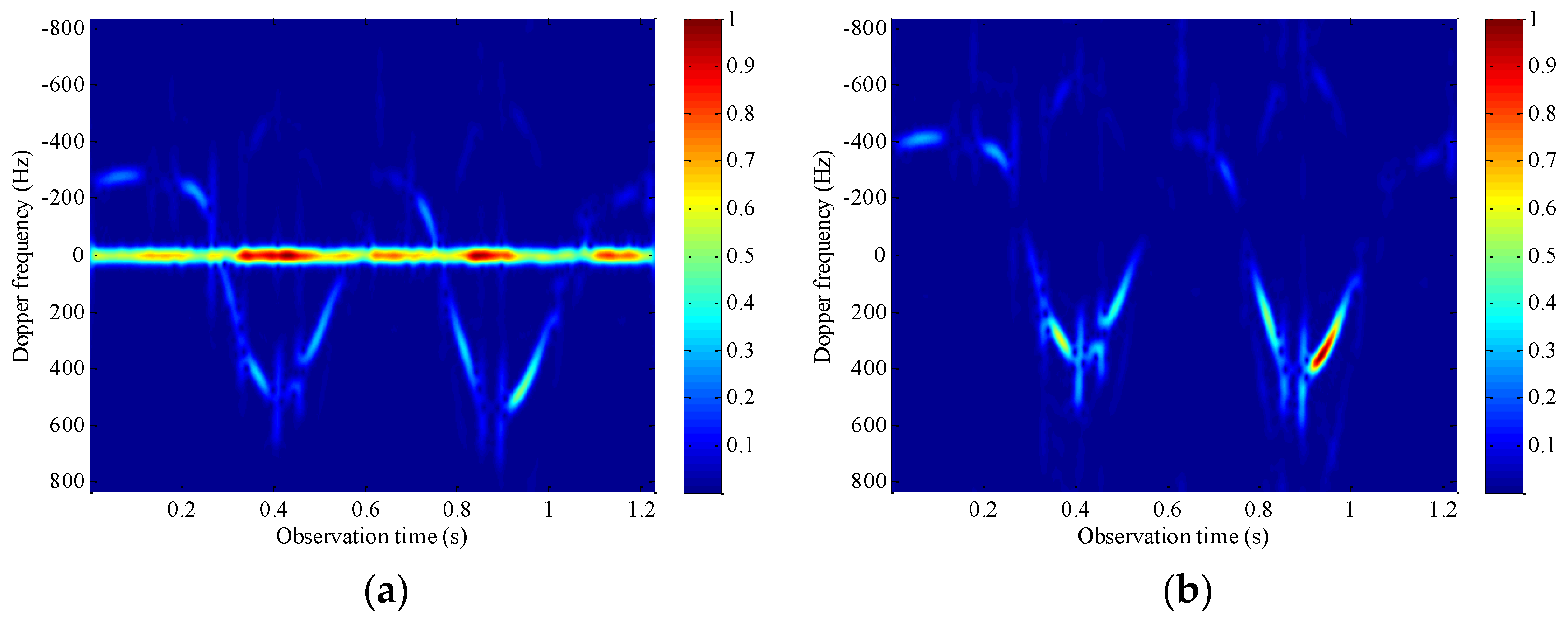
Figure 20a shows the time–frequency spectrum of the target echo. It can be seen from Figure 20 that the echo Doppler frequency of the corner reflector is approximately sinusoidal signal, which is consistent with the echo Doppler frequency of the scatterer in the theoretical derivation in this paper, which also verifies the accuracy of using this scene to simulate the real radar observation process of the rotor target. However, we can also see from the figure that the echo of the corner reflector has strong fixed ground clutter near the zero frequency, and there is translational radial motion, because the center of the sinusoidal signal is not at the zero frequency, which are all not conducive to the estimation of rotational angular velocity.

In this experiment, moving target indication processing is used to filter the clutter near zero frequency in the echo, and translational compensation is utilized to remove the influence of translational motion on the Doppler frequency of the echo, that is, the echo signal is multiplied by the translational compensation term $\exp \left(-\mathrm{j}4\mathsf{\pi }v{t}_m/\lambda \right)$, where v denotes the translational radial velocity. After these two steps of preprocessing, the time–frequency spectrum of the echo is shown in Figure 20b. Comparing Figure 20a,b, it can be found that the clutter of fixed ground objects and translational motion are basically eliminated.

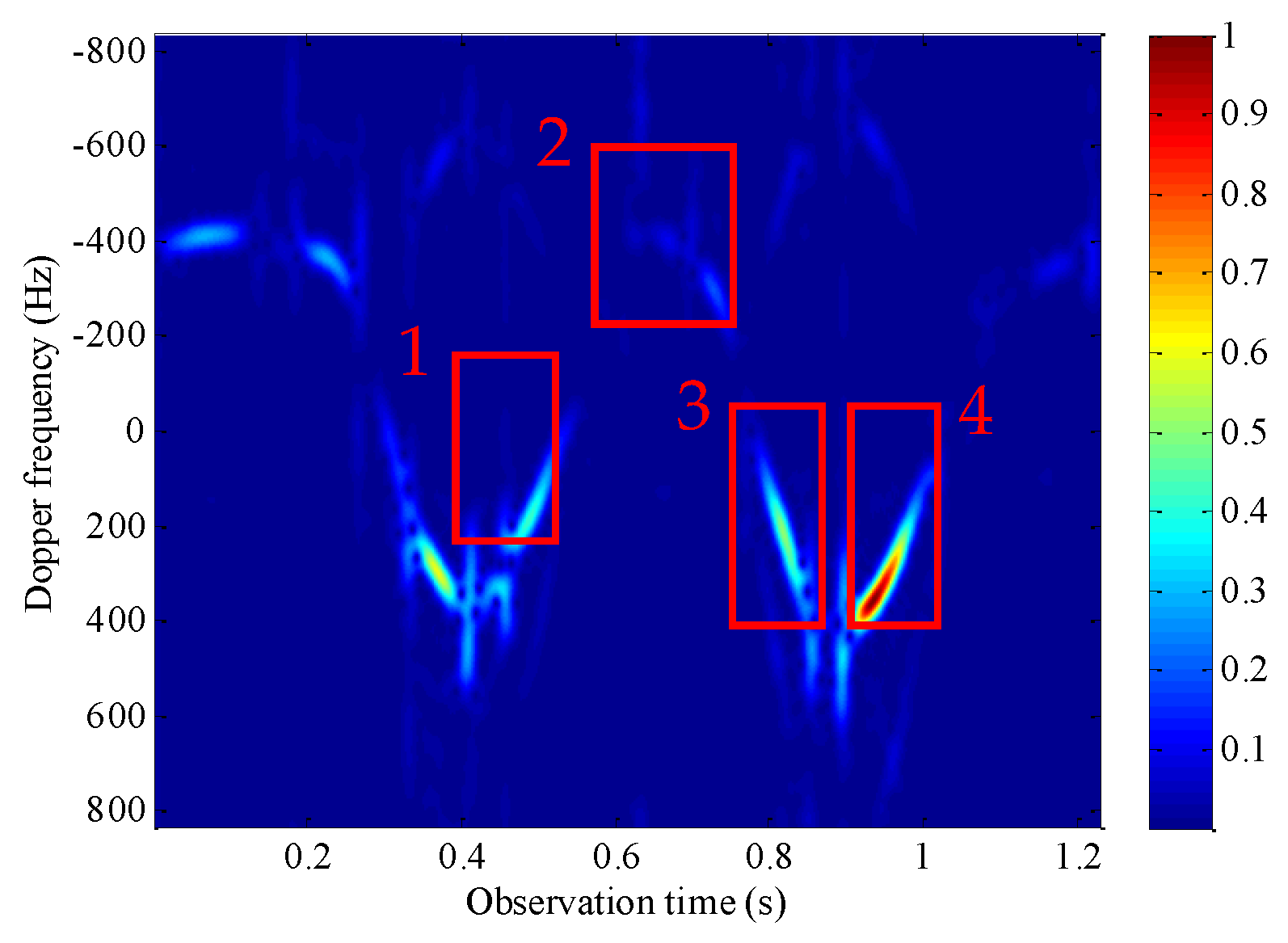
It should be pointed out that the measured data is collected on the frequency modulated continuous wave radar platform, which can realize the continuous observation of the corner reflector. However, in the actual observation process of the narrowband early warning radar on the rotor target, due to the limitation of antenna rotation and target distance, the continuous observation of the target cannot be realized. In order to simulate the real scene, we extract four effective segments from the measured data echo to verify the effectiveness of the proposed algorithm, which are shown in Figure 21 of the time–frequency spectrum marked with a red box.

Four echo segments marked with a red box in the time–frequency spectrum of Figure 21 are intercepted from the original target echo, and the rotational angular velocity of the corner reflector is estimated according to the algorithm proposed in this paper. The results are shown in

Table 2. Main steps of the OMP algorithm to reconstruct the complete entropy vector.

Algorithms	Rotational Angular Velocity (rad/s)
	Segment 1	Segment 2	Segment 3	Segment 4
Hough–STFT	15	11	11.3	12.4
Hough–WVD	14	11.6	15.7	11.7
Hough–PWVD	12	12.7	15.9	12.2
Hough–RSPWVD	12.6	12.2	15.4	12.3
Proposed algorithm	13.2	12.8	12.9	13.3

. As a comparison, the experimental results of other time–frequency analysis algorithms mentioned in Section 4.4 are given.

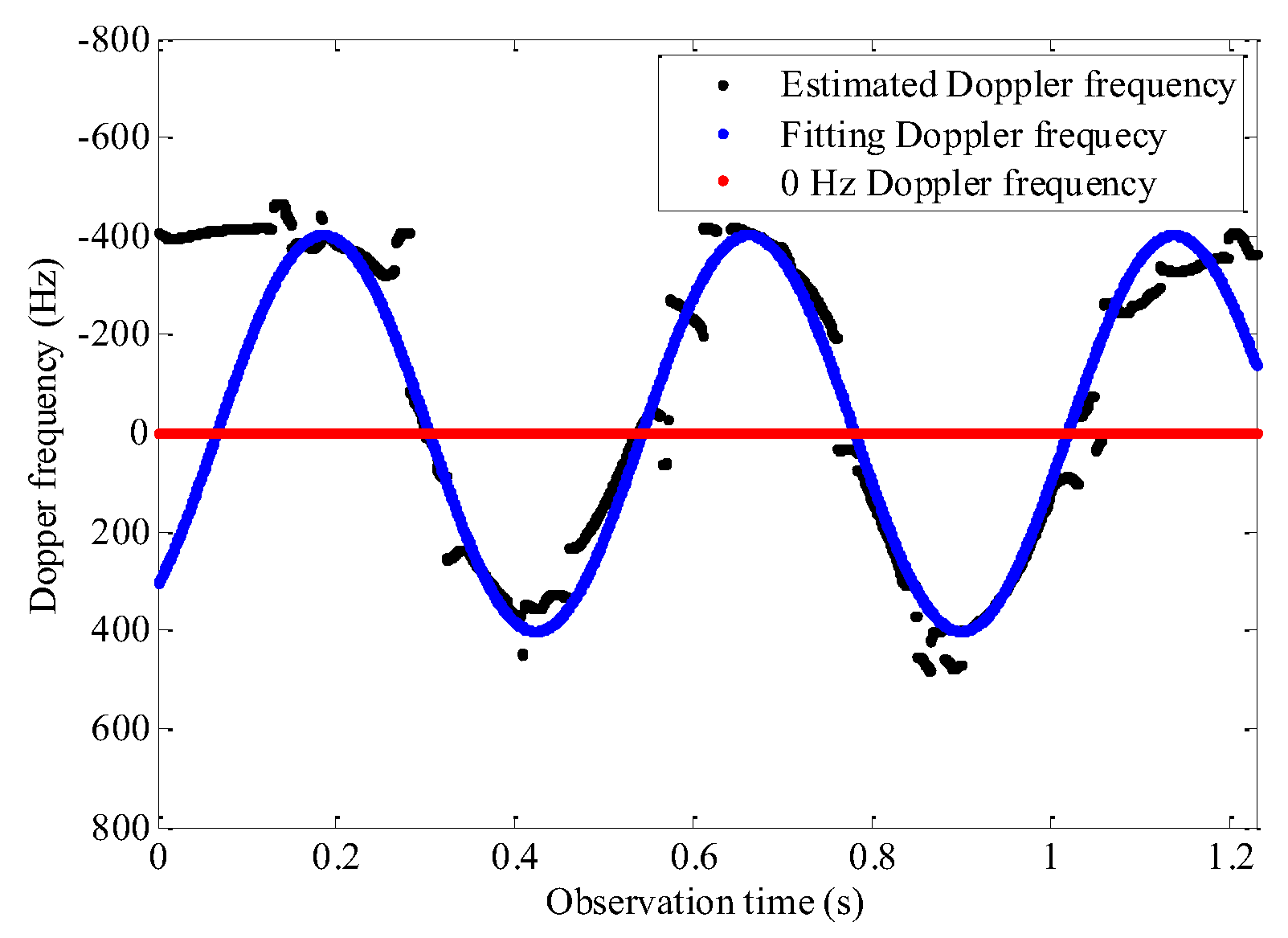
From the simulation results in Table 2, it can be seen that compared with other time–frequency analysis algorithms, the algorithm based on M-STFRFT proposed in this paper is more stable for the estimation of the rotational angular velocity of the echoes in four segments. In order to verify the correctness of the estimation results, we fit a sinusoidal Doppler frequency curve $f_d=A\sin \left(\omega t_m+\varphi \right)$, where the amplitude is A = 494, the rotational angular velocity is ω = 13.2 rad/s, and the initial phase angle is $\varphi ={131}^{°}$. The fitting result of Doppler frequency of the corner reflector is shown in Figure 22, in which the black scattered points represent the real Doppler frequency of the corner reflector estimated from the time–frequency spectrum, the red scattered points represent that the Doppler frequency value is zero, and the blue scattered points represent the fitting Doppler frequency value of the corner reflector.

According to our verification, under the Doppler frequency fitting of this group of parameters, the coincidence degree of blue scattered points and black scattered points is the highest, especially in the four segments marked in Figure 21. Therefore, it can be concluded that the rotational angular velocity of the corner reflector in the measured data is about 13.2 rad/s, which can demonstrate the correctness of the estimation results in Table 2, thus verifying the effectiveness of the algorithm proposed in this paper.

5. Conclusions

In this paper, we have presented a novel modified short-time fractional Fourier transform algorithm for efficient rotational angular velocity estimation of the rotor target. The OMP-based algorithm is used to estimate the matched transform order in the proposed M-STFRFT algorithm, and the problem of searching the maximum amplitude in FRFT is converted into the entropy minimization problem. Compared with the traditional search method, the proposed method is computationally efficient, because partial transform order candidate values are selected randomly to estimate the matched transform order through the OMP-based algorithm. The estimated matched transform order and STFRFT are applied to obtain the time–FRFD–frequency spectrum with the highest time–FRFD–frequency resolution, and the rotational angular velocity can be estimated through searching the peak value from the energy accumulation spectrum obtained by Hough transform. Simulations results demonstrate that the proposed algorithm yields better time–FRFD–frequency resolution in comparison with other mentioned time–frequency analysis algorithms, faster estimation of matched transform order than the traditional search method and more accurate rotational angular velocity estimation than the Hough–GSS-based STFRFT algorithm and other time–frequency analysis algorithms mentioned in this paper. Moreover, experimental results based on measured data collected by frequency modulated continuous wave radar validate the effectiveness of the proposed algorithm.

Although our proposed algorithm is effective in rotational angular velocity estimation, it can still be improved further. In the future, we will not only focus on the more effective estimation of the matched transform order but also verify the effectiveness of the proposed algorithm in the actual radar equipment by experimenting with measured data.