Object Tracking in Hyperspectral-Oriented Video with Fast Spatial-Spectral Features

Abstract

This paper presents a correlation filter object tracker based on fast spatial-spectral features (FSSF) to realize robust, real-time object tracking in hyperspectral surveillance video. Traditional object tracking in surveillance video based only on appearance information often fails in the presence of background clutter, low resolution, and appearance changes. Hyperspectral imaging uses unique spectral properties as well as spatial information to improve tracking accuracy in such challenging environments. However, the high-dimensionality of hyperspectral images causes high computational costs and difficulties for discriminative feature extraction. In FSSF, the real-time spatial-spectral convolution (RSSC) kernel is updated in real time in the Fourier transform domain without offline training to quickly extract discriminative spatial-spectral features. The spatial-spectral features are integrated into correlation filters to complete the hyperspectral tracking. To validate the proposed scheme, we collected a hyperspectral surveillance video (HSSV) dataset consisting of 70 sequences in 25 bands. Extensive experiments confirm the advantages and the efficiency of the proposed FSSF for object tracking in hyperspectral video tracking in challenging conditions of background clutter, low resolution, and appearance changes.

1. Introduction

Visual surveillance [1,2,3,4,5,6] is one of the most important safety monitoring and management methods widely used in various fields, such as traffic monitoring, aviation monitoring, navigation safety, and port management. In video surveillance, tracking objects of interest provides dynamic information of key objects for target monitoring and motion characteristics analysis [7,8]. We consider the most general scenario of visual tracking, single object tracking. The visual tracking task is to estimate the object state in video sequences given an initial object region in the first frame. A surveillance video obtained in an urban setting may contain highly cluttered background, making the appearance and shape of the target objects indistinguishable. Surveillance video cameras, having a broad field of view, are being used to monitor wide areas such as seaports and airports, making the imaged object appear tiny. Conventional video tracking methods relying on shape, appearance, and color information of the object [9,10] can become unreliable and are subject to tracking drift in challenging situations, including interference from similar objects, appearance changes such as deformation and illumination variations.

A hyperspectral image (HSI) [11,12] records spatial information and continuous spectral information of an object in a scene simultaneously. This has been successfully employed in the field of remote sensing and computer vision, such as super-resolution [13,14], face recognition [15,16] and object tracking [17,18]. The recently developed snapshot spectral imaging sensor [19] makes it possible to collect hyperspectral sequences at a video rate, which provides good application conditions for real-time tracking of surveillance video targets. Hyperspectral refers to much higher number of bands (to the hundreds), but the only available sensor equipment for videos with snapshot arrays at the moment can only acquire a limited number of bands. Although the collected videos contain only 25 bands per frame, the methodology developed in this work is primarily motivated for hyperspectral videos and the algorithm is highly adaptable to real-time processing of hyperspectral videos in hundreds of spectral bands. Hereafter we will simplify the discussion by calling the hyperspectral-oriented videos ‘hyperspectral videos’. Unlike traditional cameras capturing only wide-bandwidth color images, hyperspectral cameras collect many narrow bandwidth spectral images [20]. The low spectral resolution of color cameras limits their ability to classify or identify objects based on color appearance alone, while hyperspectral cameras combine the benefits of video and hyperspectral data [21]. Spectral signatures in HSI provide details on the intrinsic constitution of the material contents on the scene, which increases inter-object discrimination capability [22,23]. Therefore, hyperspectral video is more robust for distinguishing materials than conventional color video. Specifically, spectral reflectance is significantly distinguishable for objects of similar appearance and remains unchanged when the object appearances change, which improves discriminability of objects under challenging conditions, as in Figures 2 and 3 of Section 2.1.1. We further analyze the separability of whole HSI compared with RGB, and the results show that the separability of HSI is stronger than RGB images for different objects and under some challenging situations, such as appearance change, background clutter and illumination variation, as in Figures 4–7 of Section 2.1.2. Therefore, the spatial-spectral information of HSI can increase inter-object separability and discriminability to handle the tracking drift problems caused by the above challenges.

The high dimensions of HSIs are its advantage regarding discriminative ability, whereas the high dimensions will bring difficulties and high computational costs for robust feature extraction. Traditional feature extraction methods developed for RGB images may not accurately describe HSI because they do not consider spectral information [24,25]. In addition, deep features (e.g. convolution neural network (CNN) features) [26] with advanced performance in traditional tracking have high computational complexity (see Figure 1 for illustration), and the computational cost becomes higher as the number of bands increases. Existing hyperspectral tracking methods [27,28] have not fully explored spatial-spectral information and the correlation of surveillance videos collected at long distances. That is because those methods either only use spectral information or convert HSI into pseudo-color images, or are developed for videos captured from close-range scenes. They also have high computational costs, and may not be suitable for real-time surveillance video, as per the SSHMG in Figure 1. Discrimination and computational complexity of the extracted features have a great impact on tracking performance and efficiency. An effective and robust method needs to be developed to explore both spectral and spatial properties of images, which helps accurately analyze surveillance videos in real time.

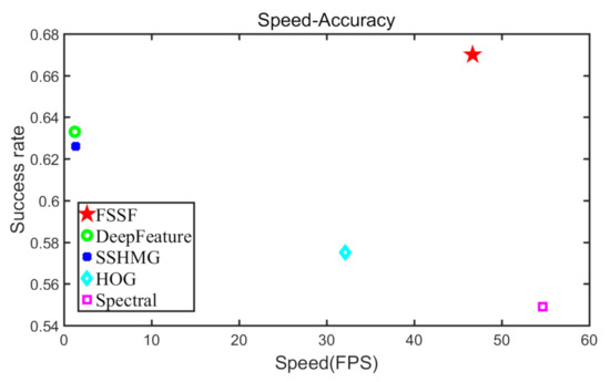
Figure 1. Tracking speed-accuracy plot of the same correlation filter tracker based on different features on a hyperspectral surveillance video (HSSV) dataset. The upper right corner indicates the best performance in terms of both standard and robust accuracy. The proposed FSSF algorithm achieves the best accuracy with faster speed.

Convolution features have been successfully employed for tracking due to their highly discriminative power in feature representations, such as deep convolution features [29]. However, the convolution kernels are generally obtained by offline iterative training of a large dataset, which has a high computation cost. Recently, some researches proposed using Fast Fourier Transforms (FFT) to reduce computational costs, which also requires offline iterative training of a large dataset [30]. High dimensions of HSIs will further increase the computational costs. Additionally, FFT-based convolution is generally more effective on larger kernels; however, the state-of-the-art deep convolution models use small kernels [31].

To solve the above problems, this paper proposes a fast spatial-spectral convolution feature (FSSF) extraction algorithm to realize object tracking in hyperspectral video with a correlation filter, which extracts discriminative spatial-spectral features from hyperspectral video in real time. The proposed FSSF develops a real-time spatial-spectral convolution (RSSC) kernel by obtaining a closed-form solution of the convolution kernel in the Fourier domain through robust ridge regression, which solves the low efficiency of existing convolution feature extraction algorithms and their requirement of large training sets. RSSC kernels can be initialized directly in the first frame and then updated in subsequent frames without offline iterative training of large dataset to extract discriminative spatial-spectral features of a HSI in real-time. The redundancy of HSI is reduced by dividing it into sub-HSIs using band correlation [32], and the weights of each sub-HSI to tracking are expressed by relative entropy. Specifically, RSSC kernels are first initialized from a set of sub-HSIs obtained from the initial frame. The initialized RSSC kernels calculate a set of features by convolving with a set of sub-HSIs obtained from subsequent frames, respectively. These features are combined to form an FSSF. Finally, the FSSF is fed to the correlation filter tracker. Different weights of sub-HSI are assigned to the correlation response maps obtained by the set of features to jointly estimate the object location and RSSC kernels are update by using the estimated object location. To validate the proposed scheme, we collected a hyperspectral surveillance video (HSSV) dataset with 70 sequences, in which each frame contains 25 bands. Extensive experiments on HSSV dataset demonstrate the advantages of hyperspectral video tracking, as well as the real-time and robustness of the proposed FSSF compared with the state-of-the-art features. Comparisons to hyperspectral trackers demonstrated the effectiveness of the FSSF-based tracker in terms of accuracy and speed. The experiments of attribute evaluation show that our method can handle typical interferences in surveillance scenes, such as low resolution, background clutter, and appearance change.

The proposed work makes three contributions:

(1)

Proposed an FSSF feature extraction algorithm to realize object tracking in hyperspectral video with a correlation filter in real time.

(2)

Developed RSSC kernels being updated in real time to encode the discriminative spatial-spectral information of each sub-HSI.

(3)

Confirmed the advantage of hyperspectral video tracking and the high efficiency and strong discriminative ability of FSSF on the collected HSSV dataset in challenging environments.

2. Related Work

2.1. Advantage Analysis of Hyperspectral Video Tracking

2.1.1. Spectral Properties of HSI

Hyperspectral imaging acquires spectral and spatial information of an object simultaneously. HSI is effective for material identification compared to visible imaging techniques [33]. The spectral spectrum captured at a pixel forms a vector of intensity values which are closely related to the material composition of objects. The objects with different material properties show substantial changes in spectral reflectance. The differences in spectral features enhance the discriminability of the target object from a cluttered background, and therefore improves tracking accuracy. Figure 2 shows the variability in spectral properties for different objects. Significant differences of spectral characteristics can be found.

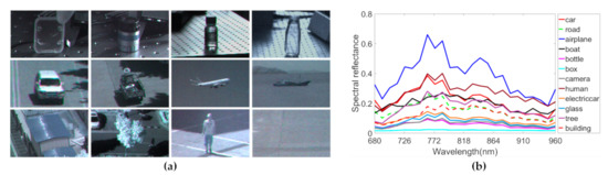
Figure 2. Spectral signatures of various materials measured at a center pixel of each object. (a) Target objects and various background materials. From left to right and top to bottom: box, camera, bottle, glass, car, electric car, airplane, boat, building, tree, human, and road. (b) Reflectance of various targets over 680-960 nm in wavelength.

In low-resolution situations, more background information is present; it is difficult to extract robust features from the target in an RGB image. However, the spectral features can be used to create robust features, which help the object stand out from surrounding environments, resulting in more accurate tracking under the small-object challenge. In the videos with in-plane-rotation, out-of-plane rotation, and occlusion attributes, although the visual quality of the target is degraded, which makes the spatial structure information unreliable, it is possible to associate the same target in the frame sequence due to intrinsic spectral properties, as shown in Figure 2.

Figure 3 shows spectral signatures of objects in challenging tracking conditions. Some examples of challenging conditions are shown in Figure 3a. Figure 3b shows spectral signatures of the same subject in two different states (normal and blurred/deformation, or exposed and shadowed). In the videos with deformation and illumination variance, there is significant variation in physical appearances of the same target in previous and subsequent frames; in RGB images, the same target will be represented by different features causing failure in tracking. However, due to the unique spectral characteristics of the target, the same object in the previous and subsequent frames can still be related. The tracker can accurately track objects with the challenge of appearance changes.

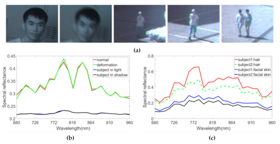
Figure 3. Sample images and their spectral reflectance. (a) Images are taken in various conditions (normal, deformation, object in shadow, object in light, and background clutter). (b) Spectral profiles of object in different states (normal, deformation and object in shadow, object in light). (c) Spectral signatures of facial skin and hair of the different subjects in the background clutter image of (a).

In the background clutter challenge, different objects may have similar appearance and color features in RGB image, for example, two pedestrians in Figure 3a. However, their spectral distributions are different. Figure 3c shows the face and hair reflectance spectra of two pedestrians in the last image of Figure 3a. Hair and facial skin show distinct hyperspectral profiles. Hence, the spectral responses perceived from the two objects address the background clutter problem of tracking.

Detailed spectral properties can increase feature discrimination. The spatial features are, naturally, additional useful information for hyperspectral video tracking. Considering the complementary advantages of spatial and spectral information, combining two kinds of information can improve traditional surveillance video tracking performance.

2.1.2. Separability Visualization of HSI

This section analyzes the separability of HSI data to further show its advantages in tracking. The dimensionality reduction can be used to visualize the multidimensional data to interpret its separability. T-SNE is one of the commonly used insightful non-linear dimensionality reduction methods for visual analysis of high-dimensional data [34]. The main idea of t-SNE is to represent multidimensional data into a low-dimensional space that can easily be visualized in scatter plots. We use t-SNE to represent the distribution of data in a two-dimensional space. Specifically, we construct four pairs of datasets as the input of t-SNE to intuitively compare the separability of HSI and RGB for different targets and under some challenging situations, such as appearance change, background clutter and illumination variation. Each category object in each dataset contains 1000 samples.

Figure 4 shows the scatter-plot representation of visualization results of the HSI and RGB datasets with multiple objects. Figure 4a is the sample images of objects in the dataset. The horizontal coordinate and vertical coordinates represent two feature values of the two-dimensional data obtained by t-SNE, respectively. Points with different colors represent the object samples from different categories and points with the same color are from different frames of the same object. The visualization results of HSIs in Figure 4b show that the intra-class data are close to each other while interclass data are far apart from each other. The different objects are well separated from each other. However, the visualization results of RGB in Figure 4c are very chaotic, and different colors of sample points are mixed and overlapped with each other.

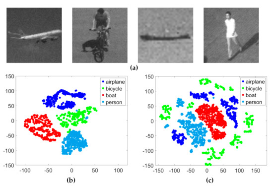
Figure 4. The scatter-plot visualization representations of different objects generated for the HSI and RGB datasets using t-SNE. (a) Sample images of the dataset (airplane, bicycle, boat, and person). (b) Visualization of the HSI dataset. (c) Visualization of the RGB dataset. The x axis and y axis represent the two feature values of the data in two-dimensional space, respectively. There are four kinds of objects, each of which is represented a particular color.

Figure 5 shows the visualization results of a two-dimensional projection of HSI and RGB datasets with deformation. Figure 5a is the sample images of the dataset with deformation. The two colors in the figure represent the normal state and deformation state of the same object, respectively. In Figure 5b, the sample points from different states are clustered in the HSI dataset; in Figure 5c, they are arranged into two categories in the RGB dataset. These results indicate that HSI data can improve the similarity of the same target in different states.

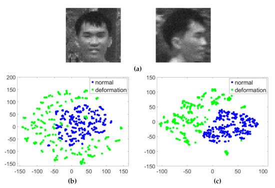
Figure 5. The scatter-plot visualization representations of the HSI and RGB datasets with the challenge of deformation using t-SNE. (a) Sample images of the dataset with deformation (normal and deformation). The target deforms as the face moves. (b) Visualization of the HSI dataset. (c) Visualization of the RGB dataset. The x axis and y axis represent the two feature values of the data in two-dimensional space, respectively. There are two states (normal and deformation) of the same object in two datasets, each of which is represented a particular color.

Figure 6 shows the visualization results of a two-dimensional projection of HSI and RGB datasets in illumination variations. Same sample images of the dataset are shown in Figure 6a. The two colors represent the light state and shadow state of the same object sample, respectively. Figure 6b is the scatter-plot of the HSI dataset, and the sample points from light and shadow states are close to each other. Figure 6c is the scatter-plot of RGB dataset, and the sample points from the two illumination states are divided into two categories. The results show that HSI data has a better ability to associate the same object under different illumination states compared to RGB data.

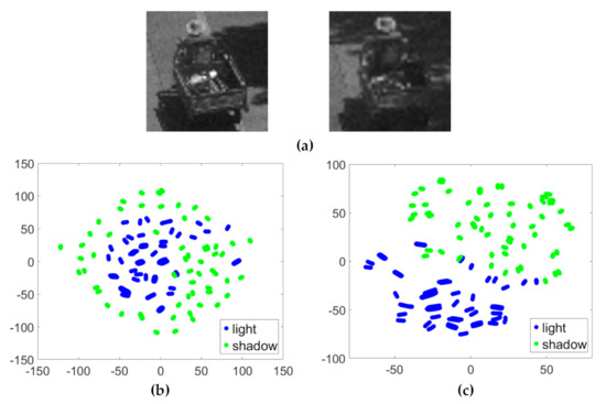
Figure 6. The scatter-plot visualization representations of the HSI and RGB datasets with the challenge of illumination variation using t-SNE. (a) Sample images of the dataset with illumination variation (object in light and object in shadow). The electric car is subjected to light changes during driving. (b) Visualization of the HSI dataset. (c) Visualization of the RGB dataset. The x axis and y axis represent the two feature values of the data in two-dimensional space, respectively. There are two states (light and shadow) of the same object in two datasets, each of which is represented by a particular color.

Figure 7 shows the visualization results of the two-dimensional projection of the HSI and RGB datasets with a background clutter challenge. Figure 7a is the sample images of the dataset. The two colors represent two objects with similar appearances, respectively. For the RGB dataset, many sample points from different categories are mixed and overlapped with each other, as in Figure 7b. For the HSI dataset, most sample points of different objects are mostly correctly arranged into two classes and the sample points of the same object are clustered into one category. Figure 7c shows that the two objects have a clear cluster structure. Namely, HSIs can separate different targets with similar appearances better than RGB data. Compared with RGB data, the spatial-spectral information of HSI data can better distinguish targets under various challenges, proving that the HSI is effective for tracking.

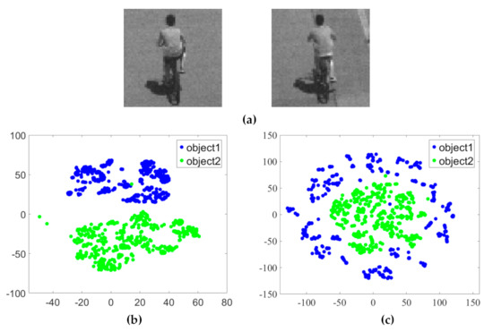
Figure 7. The scatter-plot visualization representations of the HSI and RGB datasets with the challenge of background clutter using t-SNE. (a) Sample images of the dataset with background clutter (from left to right: object1 and object2). The two objects are similar in visual appearance. (b) Visualization of the HSI dataset. (c) Visualization of the RGB dataset. The x axis and y axis represent the two feature values of the data in two-dimensional space, respectively. There are two kinds of objects in two data sets, each of which is represented by a particular color.

2.2. Hyperspectral Tracking Method

An early work of hyperspectral tracking [35] attempted to use spectral reflectance to identify pedestrians but did not take the contribution of spatial information into consideration. Uzkent et al. proposed a hyperspectral likelihood maps-aided (HLT) [36] tracker and a deep kernelized correlation filter (DeepHKCF) tracker [27]. HLT fuses likelihood maps from each band of HSI into one single, more distinctive representation. DeepHKCF converts a HSI to a pseudo-color image to extract deep convolution features. These two methods may lose valuable information and are computationally expensive. Qian et al. [37] extracts features using the 3D patches selected from an object area in the first frame, but the correlations among bands were neglected. Xiong et al. [28] proposed a spectral-spatial histogram of multi-dimensional gradients and fractional abundances of constituted material components as the object features for tracking. However, this method was developed for videos shot at close distances, and may not be suitable for aerial and marine surveillance videos collected at long distances, which would capture smaller targets. In addition, this method also has high computational complexity (see Figure 1), not suitable for real-time surveillance video tracking. Extraction of discriminative features from hyperspectral video in real-time is crucial for the overall success of object tracker, which can improve the accuracy and effectiveness of surveillance video analysis and make timely decisions.

2.3. Correlation Filter Tracking

Correlation filters have been extensively used in diverse computer vision applications such object alignment [38], recognition [39] and tracking [40]. In general, correlation filter trackers learn a correlation filter online from regions of interest of an object to infer the location of the object in consecutive frames. Correlation filters are popular due to high tracking accuracy and high computational efficiency. The correlation filter by Bolme et al. [40] has been extended to many variants such as kernel correlation filters [41,42], long-term memory [43,44,45], multi-dimensional features [46,47], part-based strategies [48,49,50], scale estimation [51,52,53], context-aware filters [54,55,56], spatial-temporal regularization [57,58,59], deep learning [60,61], and multi-feature fusion [62,63,64]. Existing correlation filter-based trackers generally follow ridge regression models. That is, the optimal correlation filter is taught by minimizing the mean squared error (MSE) between the predefined and actual output in the spatial domain:

$$h=argmin\parallel y-h\otimes x{\parallel }_2^2+\lambda \parallel h{\parallel }_2^2$$

(1)

where $x$ denotes a feature of sample, $y$ is the desired output, $\mathsf{\lambda }>0$ is the regularization parameter, and $\otimes$ is the convolution operation. Equation (1) is convex with a unique global minimum. Equating its gradient to zero, the ridge regression problem has a closed-form solution with respect to the input matrix $x$:

$$H=\left(X\ast \overline{Y}\right)/\left(X\ast X+\lambda \right)$$

(2)

where the uppercase variable denotes the Fourier transform of the corresponding lowercase letter. $\overline{X}$ and $\overline{Y}$ are complex conjugates. $\ast$ denotes elementwise multiplication. Given a new input frame, the response map is calculated using the learned H and the extracted feature $Z$ as follows:

$$y=F^{-1}\left(H\ast Z\right)$$

(3)

where $F^{-1}$ denotes the inverse Fourier transform. The object position is the location of the maximum response value. This paper combines the proposed spatial-spectral feature extraction method and correlation filter to realize hyperspectral video tracking.

3. Fast Spatial-Spectral Feature-Based Tracking

This section first describes the FSSF extraction model to extract spatial-spectral features using RSSC kernels in the Fourier domain. In FSSF extraction model, we present the problem formulation of feature extraction followed by detailed description of the initialization and updating progress of the RSSC kernels in Figure 8. After feature extraction, to jointly estimate the object location, each subset of the HSIs is assigned a weight according to relative entropy.

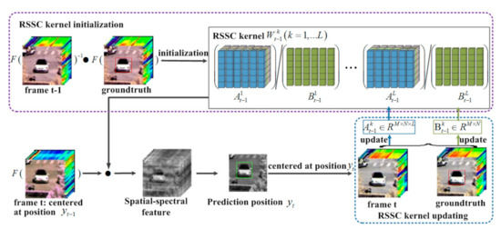
Figure 8. The initialization (purple box) and updating (blue box) process of the proposed real-time spatial-spectral convolution (RSSC) kernel. In the frame t − 1, RSSC kernels are initialized using the search region of interest centered at position $y_{t-1}$ and ground-truth bounding box of the object. For the new frame t, spatial-spectral features are extracted using the initialized RSSC kernel to estimate the object position $y_t$. Then, RSSC kernels are updated using the search region of interest and bounding box centered at $y_t$. For calculation convenience, here we update the numerator $A_t^k$ and denominator $B_t^k$ of the RSSC kernel separately. $F$ and $F^{-1}$ denote the FFT and inverse FFT, respectively.

3.1. Fast Spatial-Spectral Feature (FSSF) Extraction

3.1.1. Problem Formulation

As a common feature construction operator, a convolution kernel captures more details of spatial structures for object tracking. The features extracted from the HSI by a convolution kernel can better handle challenges, such as background clutter and deformation [65]. To effectively incorporate the spectral information into the HSI, 3D convolutional kernels are used to capture discriminative features. Formally, the feature map is given by:

$$z=x\otimes w$$

(4)

where $x\in X\times Y\times L$ is the input sample, which is the image patch centered around the target. $X\times Y$ and $L$ are the spatial resolution and the number of bands of the HSI, respectively. $w$ represents the 3D convolution kernel. $z$ means the output variable in the feature map.

The focus of feature extraction using convolution kernels is the determination of weight coefficients. The goal of training is to find an optimal convolution kernel so that the loss is close to a given threshold. The loss function is expressed as:

$$\epsilon = \parallel {\displaystyle \sum }_{i=1}^L{x}_i\otimes w_i^k-z^k\parallel$$

(5)

where $w_i^k$ are i-th dimension of k-th convolution kernel, $k\in \left\{1,\dots ,K\right\}$. ${\mathrm{z}}^k$ is the desired convolution output.

The convolution kernels are generally trained in the spatial domain using offline iterative methods. For large training datasets, the calculation cost is very high. An expedient strategy to reduce convolution computational complexity is to use Fast Fourier Transforms (FFT) [30]. In [66], filter kernel weights are converted to the frequency domain for high compression. Dziedzic et al. [67] proposed to constrain the frequency spectra of CNN kernels to reduce memory consumption. However, there are still the following problems in training the convolution kernel in FFT. A large amount of data is needed to train the convolution kernels. It is usually more efficient on a larger size of kernel for FFT-based convolution compared with a convolution operator in the spatial domain; however, the CNN models generally use a small size of kernels [31]. High dimensionality of HSIs causes a high computational cost. Therefore, the FFT-based convolution models need to be optimized for robustness and computational efficiency [68].

3.1.2. Real-Time Spatial-Spectral Convolution (RSSC) Kernel

Visual tracking requires tracking subsequent frames based on the initial frame information. Therefore, the convolution kernel can be trained from the initial frame and adapted as the appearance of the target object changes in subsequent frames. This not only can reduce training data, but the constructed convolution kernel can also be adapted to the tracking sequence, thereby making the extracted features more robust. Since ridge regression admits a simple closed-form solution, it can achieve performance close to that of more sophisticated methods. Inspired by this, we develop the RSSC kernels to extract discriminative spatial-spectral features in real-time by obtaining a closed-form solution of the convolution kernel directly in the initial frame through robust ridge regression.

We first convert the spatial domain convolution operation of feature extraction to a Fourier domain product operation. $X$and $W$ represent the Fourier transforms of $x$ and $w$respectively. $\ast$ denotes elementwise multiplication. The feature extraction problem in (4) is expressed in the Fourier domain as $z={\displaystyle \sum }_{i=1}^L{X}_i\ast W_i$. The loss function in (5) is reformulated in the Fourier domain:

$$\epsilon =\parallel {\displaystyle \sum }_{i=1}^L{X}_i\ast W_i^k-Z^k\parallel$$

(6)

In Equation (6), the optimal convolution kernel can be obtained by minimizing the error. Hence, in the Fourier domain, the iterative training problem of convolution kernels can be converted as the least squares problem. We use the ridge regression method to solve the closed-form solution of RSSC kernels. The optimal RSSC kernels are computed by minimizing the squared error between the desired output and the convolution output. Since the spatial connection of the image is local, in general, the size of the kernel is smaller than the input sample. Therefore, they need zero padding before being converted to the Fourier domain. The optimization problem takes the form:

$$\mathsf{\epsilon }=\min \parallel {\displaystyle \sum }_{i=1}^L\widehat{p}\left(X_i\right) \ast \widehat{p}\left(W_i^k\right)-{\widehat{Z}}^k{\parallel }_2^2+\lambda {\displaystyle \sum }_{k=1}^L\parallel \widehat{p}\left(W_i^k\right){\parallel }_2^2$$

(7)

where $\widehat{p}\left(X_i\right)$ and $\widehat{p}\left(W_i^k\right)$ are the Fourier forms of $x_i$ and ${\mathrm{w}}_i^k$ after zero padding, respectively, and ${\widehat{Z}}^k$ is the Fourier transformation form of $z^k$. The desired convolution output $z^k$ only includes object information. Non-zero and zero points of $z^k$ are located at the object area and background area in input sample $x$. As shown in the “ground truth” image in Figure 8, the area inside the red box is the object region, and the area outside the red box is the background region. The non-zero value of $z^k$ is the intensity value of object area in the input sample. Since different bands have different intensity values in the object area, there are $L$ desired convolution outputs corresponding to $L$ bands. The size of $z$ is the same as the input sample. $\lambda$ is the regularization term to prevent overfitting of the learned convolution kernel. The objective function in (7) can be rewritten by stacking multi-dimensional input samples with a new data matrix $\widehat{p}\left(X\right)$.

$$\mathsf{\epsilon }=\min \parallel \widehat{p}\left(X\right) \ast \widehat{p}\left(W^k\right)-{\widehat{Z}}^k{\parallel }_2^2+\lambda \parallel \widehat{p}\left(W^k\right){\parallel }_2^2$$

(8)

$\epsilon$ can be minimized by setting the gradient to zero to the solution of the k-th convolution kernel, yielding:

$$\widehat{p}{\left(W^k\right)}^T={\left(\widehat{p}{\left(X\right)}^T\widehat{p}\left(X\right)+\lambda I\right)}^{-1}\widehat{p}{\left(X\right)}^T{\widehat{Z}}^k$$

(9)

where $\widehat{p}{\left(X\right)}^T$ is the complex conjugate of $\widehat{p}\left(X\right)$.

To adapt to appearance changes caused by rotation, scale, pose and so on in the tracking process, the RSSC kernels need to be updated online to obtain robust object features in the following frames. Here the numerator $A_t$ and denominator $B_t$ of the RSSC kernel $\widehat{p}\left(W^k\right)$ are updated separately. For one RSSC kernel update, the formula is expressed as follows.

$${\widehat{p}}_{t-1}\left(W^k\right)=\frac{\widehat{p}{\left(X\right)}^T\ast Z^k}{\widehat{p}{\left(X\right)}^T\ast \widehat{p}\left(X\right)+\lambda I}=\frac{A_{t-1}^k}{B_{t-1}^k}$$

(10)

$$A_t^k=\eta {\widehat{p}}_t{\left(X\right)}^T\ast Z_t^k+\left(1-\eta \right)A_{t-1}^k$$

(11)

$$B_t^k=\eta {\widehat{p}}_t{\left(X\right)}^T\ast {\widehat{P}}_t\left(X\right)+\left(1-\eta \right)B_{t-1}^k$$

(12)

where $\eta$ is the learning rate.

The RSSC kernels in the FSSF model need only to be initialized in the first frame and updated in subsequent frames without offline training, which will reduce the computational complexity. The convolution feature can be extracted in real time. The spatial size of the RSSC kernel trained in Fourier is determined by the input image size, and the performance is not affected by the size of the convolution kernel in the spatial domain. Since the RSSC kernels are taught using the hyperspectral video sequence directly, the feature maps extracted by RSSC kernels provide efficient encoding of local spectral-spatial information of the HSI.

3.1.3. Computational Complexity Analysis

The computational time of the conventional iterative offline learning method mainly depends on the number of convolution layers, size of kernels, and the dimensions of images. Its computational complexity in the spatial domain stems from convolution operators, and is estimated at $\mathrm{O}\left({\displaystyle \sum }_{c=1}^C{L}^2{M}_c{N}_c{k}_c^2\right)$. The computational complexity in the frequency domain stems from element-wise multiplication operations and FFT, and is estimated at $\mathrm{O}\left({\displaystyle \sum }_{c=1}^{C}L{M}_c{N}_{c}logL{M}_c{N}_c\right)$. $M_c\times N_c$ is the spatial dimensions of the c-layer input image, $k_c$ is the size of the c-layer convolutional kernels, and $L$ is the spectral dimensions of the HSI. In the training process, the computational complexity of these two methods increases to $\mathrm{O}\left(D{\displaystyle \sum }_{c=1}^C{L}^2{M}_c{N}_c{k}_c^2\right)$ and $\mathrm{O}\left(D{\displaystyle \sum }_{c=1}^{C}L{M}_c{N}_{c}logL{M}_c{N}_c\right)$ with a potentially large D (iteration), respectively. Comparing the computational complexity in the two domains, the computational efficiency is improved significantly only when the size of convolution kernel is large enough. Hence, it is usually more efficient on a larger size of kernel for FFT-based convolution compared with convolution operators in the spatial domain.

Our proposed RSSC kernels can be obtained directly through regression without offline iterative learning. The complexity calculation of our method is mainly composed of element-wise multiplication and FFT. For a HSIs with size of $M\times N\times L$, since Equation (7) is separable at each pixel location, we can solve $M\times N\times s$ sub-problems, and each is a system of linear equations with $B$ variables. $B$ is the number of sub-HSIs. $s$ is the number of bands in one sub-HSI, and $L\approx B\times s$. Each system is solved in $\mathrm{O}\left(MNs\right)$. Thus, the complexity of solving $B$ RSSC kernels $w^b\left(b=1,\dots ,B\right)$ is $\mathrm{O}\left(BMNS\right)$, namely $\mathrm{O}\left(LMN\right)$. Taking the FFT, the overall complexity of our proposed online learning is $\mathrm{O}\left(LMNlog\left(MNs\right)\right)$. The number of convolutional layers is equal to 1. This indicates that our proposed method reduces computation time by several orders of magnitude compared to iterative offline learning, resulting in very fast optimization.

3.1.4. Feature Extraction

For a new frame t, we crop the region of interest from the previous frame as the input sample and convert it to the Fourier domain, and then the learned RSSC kernel $\widehat{p}{\left(W^k\right)}_{t-1}$ is convolved with the image patch $\widehat{p}{\left(X\right)}_t$. The result is the target feature representation. The feature extraction formula is given by:

$$F_t^k={\displaystyle \sum }_{i=1}^L{\widehat{p}}_t\left(X_i\right) \ast {\widehat{p}}_{t-1}\left(W_i^k\right)$$

(13)

where $F_t^k$ is the k-th dimension feature of the t-th frame in the Fourier domain. As the feature of the correlation filter tracker needs to be converted to the Fourier domain, the obtained feature does not need to be transformed back into the spatial domain.

To reduce the redundancy of the HSI, we construct sub-HSIs as the input samples by using correlation [32] between bands. Figure 9a is a visualization of the correlation coefficient matrix. We cross-group the strong correlation band images into one group, and each group forms a sub-HSI. Each sub-HSI is regressed to its desired output z to learn the corresponding RSSC kernel.

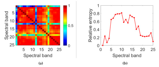
Figure 9. (a) Visualization of correlation coefficient matrix, (b) Relative entropy of each band relative to the first band.

For a given frame, the HSI is first divided into several sub-HSIs, and then the RSSC kernels are convolved with the corresponding sub-HSIs to calculate spatial-spectral features. Figure 10 visualizes the spatial-spectral feature maps of each sub-HSI in a car sequence. It shows that the object appearance and background change in different frames (first column from the left in Figure 10) of the same sequence. In this case, the spatial-spectral features are still effective in discriminating the object. It should be noted that the spatial-spectral features of various sub-HSIs are significantly different.

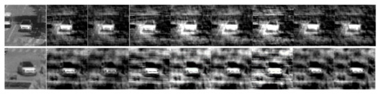
Figure 10. Visualization of the spatial-spectral feature maps extracted from different sub-HSIs. Activations are shown for two frames from the deformation challenging car sequences (left). The spatial-spectral features (right) are extracted on each sub-HSI. Notice that although the appearance of object changes significantly, we can still extract discriminative features even the background has changed dramatically.

3.2. FSSF-Based Object Tracking

Correlation filters are widely used in single object tracking due to their competitive performance and computational efficiency. Here we employ correlation filter methods as our trackers to realize hyperspectral video tracking. After the features are extracted by the FSSF extraction model from all sub-HSIs, they are fed to the correlation filter tracker to achieve object tracking. The correlation response map is obtained using Equation (3), and the maximum response is the object position estimated for the current frame. The tracking process is described in Algorithm 1. The contribution of each sub-HSI is expressed by relative entropy, which represents the difference in information. Figure 9b shows the relative entropy between each band image and the first band image. The weight of each sub-HSI can be represented by averaging the relative entropy of all band images in the sub-HSI. Finally, the object location corresponds to the location of the maximum filter response, formulated as:

$$\mathrm{y}=\max F^{-1}\left({\displaystyle \sum }_{i=1}^K{\alpha }_k\left(h_k\ast f_k\right)\right)$$

(14)

where ${\alpha }_k$ is the weight value of each sub-HSI, which is calculated by averaging the relative entropy of all band images in k-th sub-HSI.

Algorithm 1: FSSF-Based Hyperspectral Video Tracking Method

Input: t-th frame It, object position on (t − 1)-th frame $P_{t-1}$.

Output: target location on t frame $P_t$.

1:   RSSC kernel initialization:

2:   Crop an image patch $x_{t-1}$ from $I_{t-1}$ at the location on (t − 1)-th frame $P_{t-1}$, initialize convolution kernel by using (9).

3:   Repeat

4:       Location estimation

5:       Crop an image patch $x_t$ from $I_t$ centered at $P_{t-1}$.

6:       Extract the spatial-spectral feature by using (13).

7:       Compute correlation scores $y$ using (14).

8:       Set $P_t$ to the target position that maximizes $y$.

9:       RSSC kernel update:

10:     Crop a new patch $x_t$ and label $z_t$ center at $P_t$.

11:     Update RSSC kernel numerator $A_t$ by using (11), update RSSC kernel denominator $B_t$ by using (12).

12: Until end of video sequences;

4. Experimental Results

We conducted extensive experiments on proposed dataset. All trackers were performed in MATLAB on a server of Intel Core I7-7770 @3.60 GHz CPU with 16 GB RAM, and a GPU with NVIDIA GeForce GTX 1080 Ti.

4.1. Experiment Setup

4.1.1. Dataset

With the limitation of hyperspectral sensors, it is difficult to real-time collect hyper-spectral surveillance video with a wide field of view. Uzkent et al. [31] introduced a synthetic aerial hyperspectral dataset (SAHD) generated by Digital Imaging and Remote Sensing software with a low frame rate for tracking. However, this synthetic dataset is too unrealistic to cover the surveillance video tracking challenges, such as small objects, deformation, background clutter, etc. Recent advances on sensors enable collecting hyperspectral sequences at a video rate. To validate our approach, we collected a hyperspectral surveillance video (HSSV) dataset with 70 annotated sequences for object tracking. All data were captured with 25 spectral bands over visible and near infrared (680–960 nm) with a bandwidth of 10 nm using a snapshot mosaic hyperspectral camera (CMV2K SSM5*5 VIS camera) from IMEC®. This camera is hand-held and it acquires video at up to 120 hyperspectral cubes per second, making it easy to capture dynamic scenes at a video rate. Each frame of dataset is a 3D hyperspectral cube, including two-dimensional spatial position information and one-dimensional spectral band information. The captured hyperspectral dataset requires spectral calibration to remove the influence of lighting condition. We performed a white calibration to convert radiance to reflectance by normalizing the image. The spatial resolution for each band is 409 × 216. The acquisition speed and average video length of HSSV are 10 fps and 174 frames, respectively. The shortest video contains 50 frames and the longest ones consist of 600 frames. The total duration of the 70 videos for this work is 20.1 mins with 12,069 frames. Figure 11 shows an example of a HSI acquired by the hyperspectral camera. The HSSV dataset consists of three typical real-world surveillance scenarios such as aviation, navigation and traffic, where tracking targets include airplanes, ships, pedestrians, vehicles, bicycles, electric cars, and motorcycles. Some example sequences with these tracking objects are shown in Figure 12. To compare hyperspectral-based tracking and color-based tracking, we also prepared false-color videos using the three spectral bands (747.12 nm, 808.64 nm, 870.95 nm) from the hyperspectral video.

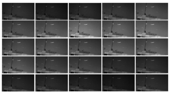
Figure 11. Illustration of a set of 25 bands of HSI. The 25 bands are ordered in ascending from left to right and top and bottom, and its center wavelengths are 682.27 nm, 696.83 nm, 721.13 nm, 735.04 nm, 747.12 nm, 760.76 nm, 772.28 nm, 784.81 nm, 796.46 nm, 808.64 nm, 827.73 nm, 839.48 nm, 849.40 nm, 860.49 nm, 870.95 nm, 881.21 nm, 889.97 nm, 898.79 nm, 913.30 nm, 921.13 nm, 929.13 nm, 936.64 nm, 944.55 nm, 950.50 nm, 957.04 nm, respectively.

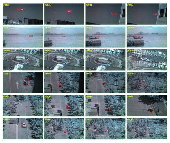
Figure 12. Example sequences with different tracking objects of the HSSV dataset. From top to bottom: airplane, boat, pedestrian, electric car, bicycle, car.

All images are annotated with high-precision bounding boxes, which are manually annotated and checked. The dataset contains various tracking challenges in actual scenarios. Each sequence is labeled with the 11 challenging attributes, including illumination variation, scale variation, occlusion, deformation, motion blur, fast motion, in-plane rotation, out-of-plane rotation, out-of-view, background clutter and low resolution. For each attribute, we construct a corresponding subset for evaluation. Each sequence usually is contained with multiple attributes. In order to reflect the advantages of hyperspectral video, some attributes occur more frequently, such as illumination variation, deformation, background clutter, low resolution, and occlusion. In summary, our collected dataset is diverse and challenging, which has the ability to comprehensively evaluate tracking methods. The full HSSV dataset will be publicly accessible.

4.1.2. Evaluation Metrics

For comparison, we assess the performance of the tracker quantitatively according to two measurements: precision rate and success rate [9]. The precision rate denotes the percentage of frames where the center location error between the predicted and actual position is less than the given threshold. The center location error is defined as $CLE=\sqrt{{\left(x1-x2\right)}^2+{\left(y1-y2\right)}^2}$ where (x1, y1) and (x2, y2) denote the central location of the predicted bounding box and the corresponding ground truth bounding box, respectively. A frame is termed as a success frame if $CLE<\xi$. $\xi$ is the given threshold, here its value is an integer from 0 to 50 pixels. The precision rate can be defined as $PR\left(\xi \right)=\frac{N_{CLE<\xi }}{N_{Total}}$ where $N_{CLE<\xi }$ is the number of frames and CLE is smaller than $\xi$, and $N_{Total}$ is the total number of image frames. The success rate is measured by the percentage of frames where the intersection over union of the predicted output and ground truth bounding box exceeds a given threshold. An intersection over union is defined as $IOU=\frac{B_t\cap B_g}{B_t\cup B_g}$, where ∩ and ∩ are the intersection and union of two regions, and $B_t$, $B_g$ denotes the area of ground truth and predicted bounding box, respectively. A frame is termed as a success frame if $IOU>\eta$. $\eta$ denotes the given threshold, with a value from 0 to 1. Therefore, the success rate can be defined as $SR\left(\eta \right)=\frac{N_{IOU>\eta }}{N_{Total}}$ where $N_{IOU>\xi }$ is the number of frames where the IOU is larger than $\eta$, and $N_{\mathrm{Total}}$ is the total number of image frames. According to different initialization strategies, we use temporal robustness evaluation (TRE), spatial robustness evaluation (SRE), and one-pass evaluation (OPE) criteria to show the precision and success rates of all the trackers. Additionally, three numerical values are further used to evaluate the performance, including distance precision (DP), overlap precision (OP) and area under curve (AUC). The fps that each tracker is able to process is discussed.

4.1.3. Comparison Scenarios

We conducted three experiments to evaluate the proposed method. First, to evaluate the advantage of hyperspectral video tracking compared to RGB tracking, we conducted the experiment using the same trackers on different inputs: spatial-spectral feature from hyperspectral video data and appearance feature from RGB data. We selected four correlation filter trackers with different feature in RGB tracking as the baseline trackers, including CN (color feature) [47], fDSST (histogram of gradients (HOG) feature) [51], ECO (HOG feature) [29], DeepECO (CNN feature) [29], STRCF (HOG feature) [57] and DeepSTRCF (CNN feature) [57]. The proposed FSSF was integrated with the selected four diverse baseline trackers, named SSCF (SS_CN, SS_fDSST, SS_ECO, and SS_STRCF). The SSCF was performed in the HSSV database, whereas the baseline trackers are performed in RGB dataset, using three bands of HSI in the HSSV dataset. The second experiment was to evaluate the effectiveness of FSSF by comparing the different feature extractors (spectral, HOG [51], CNN feature (DeepFeature) [29], SSHMG [28], and our FSSF) in the hyperspectral video. The raw spectral response was employed as a spectrum feature. The HOG feature and DeepFeature were respectively constructed by concatenating the HOG feature and DeepFeature across all the bands of a HSI. The SSHMG feature was extracted directly from the HSI. Tracking was performed based on the original ECO. The third experiment was a comparison with three hyperspectral trackers to further verify the effectiveness of proposed method.

4.2. Advantage Evaluation of Hyperspectral Video tracking

4.2.1. Quantitative Evaluation

Figure 13 illustrates the precision plot and success plot of three initialization strategies for all SSCF trackers and their baseline trackers. It clearly illustrates that all SSCF trackers perform favorably against their corresponding baselines in all three metrics, since the SSCF takes the advantages of the spatial-spectral information from HSI. It is consistent with our above expectations. Specifically, compared with DeepECO using the CNN features, SS_ECO brings an absolute improvement of 1.3% and 6.2% in the OPE metric, and 9.5% and 10.7% in TRE metric. In the SRE metric, their precision rate is equal and the success rate of SS_ECO is higher than DeepECO. Additionally, SS_STRCF performs better than DeepSTRCF by 4.0%, 1.2% and 2.6% in precision rate, and 5.1%, 5.0% and 6.9% in success rate, in three metrics respectively. Compared with fDSST and CN with hand-crafted features, spatial-spectral information of HSIs increases the tracking performance by 13.9% and 4.0% in precision rate respectively, and 13.7% and 5.7% in success rate respectively, in the TRE metric.

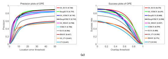
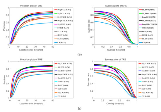
Figure 13. Comparison results for all SSCF trackers and their baseline trackers using three initialization strategies: one-pass evaluation (OPE), temporal robustness evaluation (TRE) and spatial robustness evaluation (SRE). (a) Precision plot and the success plot on OPE. (b) Precision plot and the success plot on SRE. (c) Precision plot and the success plot on TRE. The legend of precision plots and success plots report the precision scores at a threshold of 20 pixels and area-under-the-curve (AUC) scores, respectively.

Table 1 shows the results of OP with a threshold of 0.5, and their tracking speed. SSCF trackers perform well compared to their corresponding baseline trackers. The best tracker, SS_ECO, surpasses its corresponding baseline tracker DeepECO by 8.1 %. These results indicate that hyperspectral information is beneficial to increase feature representation ability compared to RGB images. Our SSCF can extract discriminative spatial-spectral features, resulting in a robust tracker. Thus, our method achieves better performance than other baseline trackers, which use RGB datasets from HSSV datasets.

Table 1. Mean overlap precision (OP) metric (in %) and fps of our SSCF and their corresponding baseline trackers.

	SS_STRCF	DeepSTRCF	STRCF	SS_ECO	DeepECO	ECO	SS_fDSST	fDSST	SS_CN	CN
Mean OP	0.775	0.719	0.680	0.829	0.748	0.592	0.704	0.453	0.463	0.395

4.2.2. Attribute-Based Evaluation

This section analyzes the tracking performance under different attributes to better highlight the advantages of hyperspectral video in tracking. Figure 14 shows the success rate plots for eight attributes. We can observe that SSCF trackers perform better under the challenges of background clutter, deformation, illumination variation, low resolution, occlusion, out-of-plane rotation, out-of-view, and scale variation. Specifically, SSCF improves significantly for videos with low resolution. The main reason is that the object is too small and contains less appearance or color information, hence, it is difficult to extract discriminative features from a RGB image. In contrast, FSSF can represent internal attribute information, which can increase the feature discrimination of small targets. On the out-of-plane rotation, deformation and out-of-view subsets, the spatial structure feature is unreliable. Therefore, baseline trackers that only use appearance information have poor performance. Benefiting from spectral information, SSCF tracker is robust to such kinds of variations. On the background clutter subset, our method provides much better results. This is mainly due to the fact that spectral information can distinguish the target from a background that has a similar color and appearance. As for occlusion, out-of-view and scale variation attributes, SSCF also performs better, which suggests that spatial-spectral representation is more effective in dealing with scale variation and occlusion compared to RGB representation.

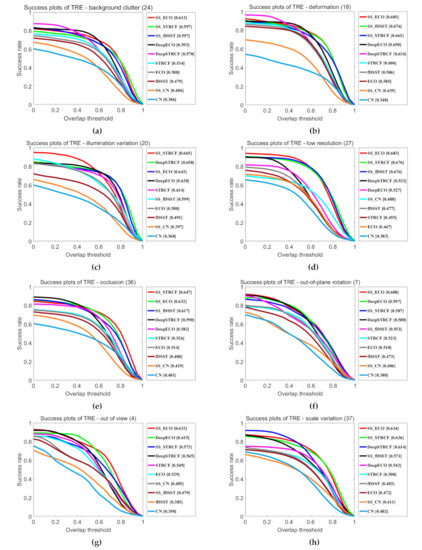
Figure 14. Success plots over eight tracking attributes, including (a) background clutter (24), (b) deformation (18), (c) illumination variation (20), (d) low resolution (27), (e) occlusion (36), (f) out-of-plane rotation (7), (g) out of view (4), (h) scale variation (37). The values in parentheses indicate the number of sequences associated with each attribute. The legend reports the area-under-the-curve score.

4.2.3. Qualitative Evaluation

To visualize the advantage of hyperspectral video tracking, Figure 15 shows a qualitative evaluation of SSCF trackers compared to their baseline trackers (from top to bottom, CN, fDSST, DeepECO, DeepSTRCF) under the challenges of deformation, low resolution, in-plane rotation, illumination variation, background clutter and occlusion. Detailed analysis is as follows.

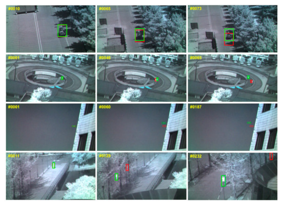
Figure 15. Qualitative results of our hyperspectral video compared to traditional video on some challenging sequences (electriccar, double5, airplane9, human4). The results of SSCF tracker and the baseline tracker are represented by green and red boxes, respectively.

In Figure 15, for the electriccar sequence involving illumination variation, SS_CN performs better than CN in terms of locating the target. This is because the object color or appearance will change in the illumination variation case while the spectral information from a HSI does not. In the double5 sequence, involving background clutter, deformation and in-plane rotation, the tracking results of fDSST will drift to the similar object because the HOG features of the similar target are similar, as shown in frames #46 and #65. However, since spectral information of hyperspectral video can handle the deformation challenge, SS_fDSST still tracks the object accurately. In the airplane9 sequence, DeepECO loses the target at the final stage (e.g. #187). Nevertheless, SS_ECO still performs well because hyperspectral video provides additional spectral information for small objects. In the human4 sequence, the person undergoes occlusion by a tree. The DeepSTRCF tracker cannot capture the target through the entire sequence. The features extracted from HSI still have high discrimination power under occlusion situations, so SS_STRCF locates the target successfully.

4.2.4. Running Time Evaluation

Tracking speed is an important factor of real-time tracking. Table 2 shows the FPS comparison of our SSCF and their corresponding baseline trackers. In Table 2, the two SSCF trackers with the best performance, SS_ECO and SS_STRCF, have greatly improved tracking speed compared to their corresponding baseline trackers. Specifically, SS_ECO runs at around 46.68 fps on CPU, which is nearly 4 times faster than its corresponding tracker DeepECO with deep features that runs with a GPU. SS_STRCF runs at around 23.64 fps on CPU, which is more than 4 times faster than its corresponding baseline tracker DeepSTRCF (deep feature) which runs at 5.73 fps (gpu). We also compare the computation time between our spatial-spectral feature FSSF and RGB feature (deep feature, hog feature and color feature) in Table 3. For fair comparison, all the features are integrated into the same tracker, STRCF. In Table 3, our FSSF feature is slightly slower than HOG, close to color feature, and far greater than deep feature in terms of computation time of tracking. In summary, performance gain and tracking efficiency of the spatial-spectral feature are both achieved compared to the spatial feature from an RGB image.

Table 2. FPS of our SSCF and their corresponding baseline trackers.

	SS_STRCF	DeepSTRCF	STRCF	SS_ECO	DeepECO	ECO	SS_fDSST	fDSST	SS_CN	CN
FPS	23.64(cpu)	5.73(gpu)	32.11	46.68(cpu)	11.87(gpu)	67.58	45.8985	220.30	126.17	981.94

Table 3. FPS comparison between spatial feature and spatial-spectral feature with same tracker.

	Spatial-Sepctral Feature	Spatial Feature
	FSSF	DeepFeature	HOG	Color
FPS	23.64	5.73(gpu)	32.11	24.0113

4.3. Effectiveness Evaluation of Proposed FSSF

4.3.1. Quantitative Evaluation

Figure 16 shows the comparison results in three indexes. The spectral feature provide the worst accuracy among all the compared methods, as the raw spectrum is sensitive to illumination changes. However, it has the fastest tracking speed among all the compared features. The HOG feature considers the local spatial structure information which is crucial for object tracking, and therefore produces more favorable results. However, the complete spectral-spatial structural information in an HSI is not fully explored. Compared to the HOG-based tracker, FSSF achieves a gain of 5.7%, 4.7% and 3.1% in precision rate, and 9.5%, 6.9% and 7.2% in the success rate, in three indexes respectively. Compared to DeepFeature, FSSF performs better in the success rate of all three indexes. For precision rate, FSSF has better precision in all three indexes when the location error threshold is less than 10 pixels. This is due to the fact that the DeepFeature is constructed by concatenating the DeepFeature across all the bands of an HSI, without considering the spectral correlation of bands. The strong correlation between the spectral bands makes the extracted DeepFeature redundant, resulting an inaccurate bounding box of the target. We also report the mean DP (MDP) and mean OP (MOP) at various thresholds where the overlap threshold is greater than 0.5 and distance threshold is less than 20 in Table 4. The MDP and MOP of our method are higher than the DeepFeaure in all setting thresholds, which suggests that our FSSF predicts a more accurate bounding box than DeepFeature. Compared with SSHMG, the precision rate and success rate of FSSF are both higher and obtain the gain of 3.4%, 2.2% and 3.5% in the precision rate, and 4.4%, 2.4% and 4.8% in the success rate, in three indexes respectively. The main reason for this result is that SSHMG describes the local spectral spatial structure information of the target, which is not available for the small objects existed in the surveillance video. For tracking speed, our FSSF runs at around 48.08 fps on the CPU, which is nearly 34 times faster than DeepFeature running on the GPU and 33 times faster than SSHMG. Our method brings a significant improvement in computational efficiency when compared to DeepFeature and advanced HSI feature. In summary, our proposed FSSF extraction model can quickly extract more discriminative spatial-spectral features from HSI at a low computational cost.

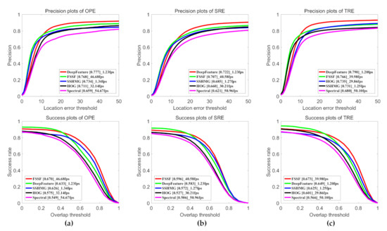
Figure 16. Precision and success plot of different features on a HSSV dataset using three initialization strategies: one-pass evaluation (OPE), temporal robustness evaluation (TRE) and spatial robustness evaluation (SRE). (a) Precision plot and the success plot on OPE. (b) Precision plot and the success plot on SRE. (c) Precision plot and the success plot on TRE. The legend of precision plots and success plots report the precision scores at a threshold of 20 pixels and area-under-the-curve scores, respectively. The fps of trackers in three initialization strategies is also shown in legend.

Table 4. Mean DP (MDP) and mean OP (MOP) in different threshold and fps of FSSF versus DeepFeature. MDP (20) denotes the mean DP (% at pixel distance <20). MOP (0.5) denotes the mean OP (% at IOU > 0.5).

Attribute	MDP(20)	MDP(15)	MDP(10)	MDP(5)	MOP(0.5)	MOP(0.6)	MOP(0.7)	MOP(0.8)	fps
FSSF	0.620	0.558	0.457	0.265	0.471	0.395	0.298	0.178	46.68
DeepFeature	0.594	0.510	0.378	0.178	0.385	0.303	0.214	0.116	1.23

4.3.2. Attribute-Based Evaluation

The effectiveness of the proposed FSSF is further verified by analyzing the tracking performance under different challenges. Figure 17 shows the tracking results in success plot of six attributes. FSSF shows significant superior performance than the spectral feature and HOG feature in all six attributes due to spectral feature only consider spectral information and HOG feature describes spatial structure information only at each band. Additionally, FSSF performs better than SSHMG in all six challenges, especially low resolution, occlusion and fast motion, which achieved improvements of 5.7%, 5.3% and 10.6% respectively. The hand-craft feature SSHMG describes the local spatial-spectral texture structure, which is unreliable due to less target information and rapid appearance changes under these challenges. However, our FSSF will update in real time according to the change of the target. Compared to DeepFeature, FSSF provides a gain of 8.7% and 2.7% in mean success rate in low resolution and occlusion, respectively. As for the challenges of scale variation, fast motion, the success rate of FSSF is slightly higher success rate than the DeepFeature. In the background clutter and deformation attributes, FSSF exhibits much better performance than DeepFeature when the threshold of the evaluation indicator is high.

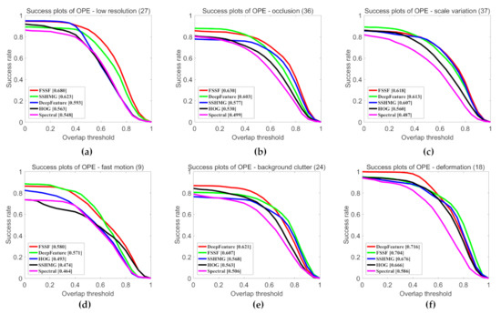
Figure 17. Success plots over six tracking attributes, including (a) low resolution (27), (b) occlusion (36), (c) scale variation (37), (d) fast motion (9), (e) background clutter (24), (f) deformation (18). The values in parentheses indicate the number of sequences associated with each attribute. The legend reports the area-under-the-curve score.

We also report the comparison results in Mean OP score at the IOU>0.5 in Table 5. The results show that FSSF ranks the first on 8 out of 11 attributes: low resolution, background clutter, occlusion, scale variation, deformation, in-plane rotation, out-of-plane rotation, and fast motion. In the low resolution and background clutter situations, the object has less appearance information or there is similar interference, the CNN model trained by RGB dataset cannot fully extract the spectral features of an object. The proposed FSSF makes full use of hyperspectral information, which is beneficial for correlating the same object in the sequence. On the videos with occlusion, scale variation, deformation, in-plane rotation, out-of-plane rotation, and fast motion attributes, the results demonstrate that FSSF still can provide discriminative features, suppressing the influence of object changes during tracking. In summary, the proposed FSSF is capable of accurately tracking objects in the challenges of low resolution, occlusion, scale variation, background clutter, deformation, and fast motion.

Table 5. Attribute-based comparison with DeepFeature in terms of mean OP (% at IOU>0.5). The best results are shown in bold, our FSSF ranks the first on 8 of 11 attributes: low resolution, background clutter, occlusion, out-of-plane rotation, in-plane rotation, fast motion, scale variation, and deformation.

Attribute	FSSF	DeepFeature
Illumination variation	0.520	0.530
Scale variation	0.419	0.388
Occlusion	0.442	0.373
Deformation	0.506	0.468
Motion blur	0.444	0.473
Fast motion	0.349	0.315
In-plane rotation	0.392	0.317
Out-of-plane rotation	0.378	0.369
Out-of-view	0.357	0.372
Background clutter	0.439	0.409
Low resolution	0.450	0.287

4.4. Comparison With Hyperspectral Trackers

4.4.1. Quantitative Evaluation

This section compares the proposed method to the recent hyperspectral trackers HLT [36], DeepHKCF [27], MHT [28]. Figure 18 shows the comparison results. We can observe that our SSCF tracker is among the top performers in terms of both precision and success rate. HLT tracker is the lowest in terms of both precision and success rates due to the fact that it uses hand-craft feature and SVM classifier. The DeepHKCF provides a gain of 24.6% in precision rate and 24.2% in success rate compared to HLT since it learns discriminative CNN features by using the VGGNet and tracks objects utilizing the KCF-based tracker, which are both more robust than hand-craft features and SVM for tracking. However, DeepHKCF uses false color images obtained by HSIs to extract the CNN features, which cannot fully explore the spatial-spectral structural information. In contrast, our SS-ECO and MHT methods obtain better performance than DeepHKCF since they extract the spatial-spectral features from the HSI. The proposed method shows higher performance than MHT. The average precision rate and success rate are higher by an average of 3.4% and 4.4%, respectively. The main reason is that MHT uses the local spatial-spectral structure features, which are not unreliable for small objects and targets with rapid appearance changes in surveillance videos. In contrast, our method can update the feature extractor in real-time to adapt to the various changes of objects in tracking.

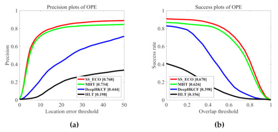
Figure 18. Comparison results with hyperspectral trackers. (a) Precision plot. (b) Success plot. The legend of the precision plot and success plot report the precision scores at a threshold of 20 pixels and area-under-the-curve (AUC) scores, respectively.

Table 6 shows the comparison of DP and OP using the threshold of 20 pixels and 0.5, respectively. We can observe that the performance of SS_ECO is more than 2 times and 5 times better than the DeepHKCF and HLT. SS_ECO achieves OP and DP of 83.2% and 82.9%, which provides a gain of 2.6% and 4.1% compared with MHT. This is consistent with the results of Figure 18. For the tracking speed, the fps of our method is nearly 35 times higher than the second ranked tracker MHT.

Table 6. Mean OP, DP metric (in %) and fps of SSCF and hyperspectral trackers.

	SS_ECO	MHT	DeepHKCF	HLT
Mean OP	0.520	0.506	0.444	0.349
Mean DP	0.829	0.788	0.375	0.110
FPS	46.68	1.34	49.87	1.58

4.4.2. Attribute-Based Evaluation

We further analyze some common challenging factors in tracking. Table 7 lists AUC metrics for three trackers in all challenges. We can observe that SS_ECO performs well in all scenarios. HLT has the worst tracking performance on all attributes since it only uses spectral information as features. SS_ECO has a margin of 11.7–36.9% in success rate (11.7% in in-plane rotation, 36.9% in illumination variation) over DeepHKCF on all attributes. The main reason for this result is that the pseudo-color videos lose the beneficial spectral information for tracking. Additionally, SS_ECO outperforms MHT in all challenges, especially under the challenges of low resolution, illumination variation, occlusion, motion blur, fast motion, and out-of-view; the gains of SS_ECO are all more than 5% compared with the second-best tracker, MHT. Table 7 demonstrates that the proposed method can extract discriminative spatial-spectral features to handle various challenges effectively.

Table 7. Attribute-based comparison with hyperspectral trackers in the term of AUC. The best results are shown in bold.

Attribute	SS_ECO	MHT	DeepHKCF	HLT
Illumination variation	0.658	0.578	0.289	0.147
Scale variation	0.618	0.607	0.387	0.146
Occlusion	0.630	0.577	0.391	0.152
Deformation	0.704	0.676	0.395	0.129
Motion blur	0.641	0.555	0.434	0.087
Fast motion	0.580	0.474	0.389	0.126
In-plane rotation	0.596	0.591	0.479	0.178
Out-of-plane rotation	0.623	0.586	0.437	0.076
Out-of-view	0.574	0.407	0.419	0.158
Background clutter	0.607	0.568	0.362	0.151
Low resolution	0.680	0.623	0.388	0.105

5. Conclusions

This paper presents object tracking in hyperspectral video using a fast spatial-spectral feature (FSSF)-based tracking method. The FSSF-based tracker extracts discriminative spatial-spectral features in real time with real-time spatial-spectral convolution (RSSC) kernels in the Fourier transform domain to overcome the challenges of traditional surveillance video tracking for real-time and accurate hyperspectral video tracking. To evaluate the proposed method, we collected a HSSV tracking dataset. Extensive experiments on the collect HSSV dataset demonstrate the advantage of hyperspectral video tracking in several challenging conditions and the high efficiency and strong robustness of the proposed FSSF-extraction model.

Due to the robustness and real-time performance of the proposed method, hyperspectral surveillance can improve the accuracy of surveillance video analysis and the proposed tracker can be successfully used in various surveillance applications. In further work, we will further develop more robust hyperspectral features by exploring the spatial-temporal context information, feature attention mechanisms and high-level semantic information. On the other hand, the improvement of tracking methods also will significantly increase the accuracy and real-time of surveillance video analysis.

References

- Shao, Z.; Wang, L.; Wang, Z.; Du, W.; Wu, W. Saliency-Aware Convolution Neural Network for Ship Detection in Surveillance Video. IEEE Trans. Circuits Syst. Video Technol. 2019, 30, 781–794. [Google Scholar] [CrossRef]
- Zhou, J.T.; Du, J.; Zhu, H.; Peng, X.; Liu, Y.; Goh, R.S.M. AnomalyNet: An anomaly detection network for video surveillance. IEEE Trans. Inf. Forensics Sec. 2019, 14, 2537–2550. [Google Scholar] [CrossRef]
- Hu, L.; Ni, Q. IoT-driven automated object detection algorithm for urban surveillance systems in smart cities. IEEE Internet Things J. 2018, 5, 747–754. [Google Scholar] [CrossRef]
- Li, A.; Miao, Z.; Cen, Y.; Zhang, X.-P.; Zhang, L.; Chen, S. Abnormal event detection in surveillance videos based on low-rank and compact coefficient dictionary learning. Pattern Recognit. 2020, 108, 107355. [Google Scholar] [CrossRef]
- Ye, L.; Liu, T.; Han, T.; Ferdinando, H.; Seppänen, T.; Alasaarela, E. Campus Violence Detection Based on Artificial Intelligent Interpretation of Surveillance Video Sequences. Remote Sens. 2021, 13, 628. [Google Scholar] [CrossRef]
- Li, M.; Cao, X.; Zhao, Q.; Zhang., L.; Meng., D. Online Rain/Snow Removal from Surveillance Videos. IEEE Trans. Image Process. 2021, 30, 2029–2044. [Google Scholar] [CrossRef] [PubMed]
- Zhang, P.; Zhuo, T.; Xie, L.; Zhang, Y. Deformable object tracking with spatiotemporal segmentation in big vision surveillance. Neurocomputing 2016, 204, 87–96. [Google Scholar] [CrossRef]
- Zou, Q.; Ling, H.; Pang, Y.; Huang, Y.; Tian, M. Joint Headlight Pairing and Vehicle Tracking by Weighted Set Packing in Nighttime Traffic Videos. IEEE Trans. Intell. Transp. Syst. 2018, 19, 1950–1961. [Google Scholar] [CrossRef]
- Müller, M.; Bibi, A.; Giancola, S.; Alsubaihi, S.; Ghanem, B. TrackingNet: A large-scale dataset and benchmark for object tracking in the wild. In Proceedings of the 2018 IEEE Conference on Computer Vision and Pattern Recognition, CVPR 2018, Salt Lake City, UT, USA, 18–22 June 2018. [Google Scholar]
- Stojnić, V.; Risojević, V.; Muštra, M.; Jovanović, V.; Filipi, J.; Kezić, N.; Babić, Z. A Method for Detection of Small Moving Objects in UAV Videos. Remote Sens. 2021, 13, 653. [Google Scholar] [CrossRef]
- Yang, J.; Zhao, Y.-Q.; Chan, J.C.-W. Hyperspectral and Multispectral Image Fusion via Deep Two-Branches Convolutional Neural Network. Remote Sens. 2018, 10, 800. [Google Scholar] [CrossRef]
- Xie, F.; Gao, Q.; Jin, C.; Zhao, F. Hyperspectral Image Classification Based on Superpixel Pooling Convolutional Neural Network with Transfer Learning. Remote Sens. 2021, 13, 930. [Google Scholar] [CrossRef]
- Yang, J.; Zhao, Y.Q.; Chan, J.C.W.; Xiao, L. A Multi-Scale Wavelet 3D-CNN for Hyperspectral Image Super-Resolution. Remote Sens. 2019, 11, 1557. [Google Scholar] [CrossRef]
- Xue, J.; Zhao, Y.-Q.; Bu, Y.; Liao, W.; Chan, J.C.-W.; Philips, W. Spatial-Spectral Structured Sparse Low-Rank Representation for Hyperspectral Image Super-Resolution. IEEE Trans. Image Process. 2021, 30, 3084–3097. [Google Scholar] [CrossRef] [PubMed]
- Uzair, M.; Mahmood, A.; Mian, A. Hyperspectral Face Recognition With Spatiospectral Information Fusion and PLS Regression. IEEE Trans. Image Process. 2015, 24, 1127–1137. [Google Scholar] [CrossRef] [PubMed]
- Shen, L.; Zheng, S. Hyperspectral face recognition using 3D Gabor wavelets. In Proceedings of the 5th International Conference on Pattern Recognition and Machine Intelligence PReMI 2013, Kolkata, India, 10–14 December 2013. [Google Scholar]
- Uzkent, B.; Hoffman, M.J.; Vodacek, A. Real-Time Vehicle Tracking in Aerial Video Using Hyperspectral Features. In Proceedings of the 2016 IEEE Conference on Computer Vision and Pattern Recognition Workshops (CVPRW), Las Vegas, NV, USA, 26 June–1 July 2016. [Google Scholar]
- Tochon, G.; Chanussot, J.; Dalla Mura, M.; Bertozzi, A.L. Object Tracking by Hierarchical Decomposition of Hyperspectral Video Se-quences: Application to Chemical Gas Plume Tracking. IEEE Trans. Geosci. Remote Sens. 2017, 55, 4567–4585. [Google Scholar] [CrossRef]
- Sofiane, M. Snapshot Multispectral Image Demosaicking and Classification. Ph.D. Thesis, University of Lille, Lille, France, December 2018. [Google Scholar]
- Ye, M.; Qian, Y.; Zhou, J.; Tang, Y.Y. Dictionary Learning-Based Feature-Level Domain Adaptation for Cross-Scene Hyperspectral Image Classification. IEEE Trans. Geosci. Remote Sens. 2017, 55, 1544–1562. [Google Scholar] [CrossRef]
- Al-Khafaji, Z.J.; Zia, A.; Liew, A.W.-C. Spectral-spatial scale invariant feature transform for hyperspectral images. IEEE Trans. Image Process. 2018, 27, 837–850. [Google Scholar] [CrossRef]
- Liang, J.; Zhou, J.; Tong, L.; Bai, X.; Wang, B. Material based salient object detection from hyperspectral images. Pattern Recognit. 2018, 76, 476–490. [Google Scholar] [CrossRef]
- Uzkent, B.; Hoffman, M.J.; Vodacek, A. Integrating Hyperspectral Likelihoods in a Multidimensional Assignment Algorithm for Aerial Vehicle Tracking. IEEE J. Sel. Top. Appl. Earth Obs. Remote Sens. 2016, 9, 4325–4333. [Google Scholar] [CrossRef]
- Zha, Y.; Wu, M.; Qiu, Z.; Sun, J.; Zhang, P.; Huang, W. Online Semantic Subspace Learning with Siamese Network for UAV Tracking. Remote Sens. 2020, 12, 325. [Google Scholar] [CrossRef]
- Sun, M.; Xiao, J.; Lim, E.G.; Zhang, B.; Zhao, Y. Fast Template Matching and Update for Video Object Tracking and Segmentation. In Proceedings of the 2020 IEEE/CVF Conference on Computer Vision and Pattern Recognition (CVPR), Seattle, WA, USA, 16–18 June 2020. [Google Scholar]
- Lukezic, A.; Vojir, T.; Zajc, L.C.; Matas, J.; Kristan, M. Discriminative Correlation Filter with Channel and Spatial Reliability. In Proceedings of the 2017 IEEE Conference on Computer Vision and Pattern Recognition (CVPR), Honolulu, HI, USA, 21–26 July 2017. [Google Scholar]
- Uzkent, B.; Rangnekar, A.; Hoffman, M.J. Tracking in Aerial Hyperspectral Videos Using Deep Kernelized Correlation Filters. IEEE Trans. Geosci. Remote Sens. 2019, 57, 449–461. [Google Scholar] [CrossRef]
- Xiong, F.; Zhou, J.; Qian, Y. Material Based Object Tracking in Hyperspectral Videos. IEEE Trans. Image Process. 2020, 29, 3719–3733. [Google Scholar] [CrossRef]
- Danelljan, M.; Bhat, G.; Khan, F.S.; Felsberg, M. ECO: Efficient convolution kernels for tracking. In Proceedings of the Conference on Computer Vision Pattern Recognition, Honolulu, HI, USA, 21–26 July 2017. [Google Scholar]
- Brosch, T.; Tam, R. Efficient Training of Convolutional Deep Belief Networks in the Frequency Domain for Application to High-Resolution 2D and 3D Images. Neural Comput. 2015, 27, 211–227. [Google Scholar] [CrossRef] [PubMed]
- Xu, K.; Qin, M.; Sun, F.; Wang, Y.; Chen, Y.-K.; Ren, F. Learning in the Frequency Domain. In Proceedings of the 2020 IEEE/CVF Conference on Computer Vision and Pattern Recognition (CVPR), Seattle, WA, USA, 16–18 June 2020. [Google Scholar]
- Wei, X.; Zhu, W.; Liao, B.; Cai, L. Scalable One-Pass Self-Representation Learning for Hyperspectral Band Selection. IEEE Trans. Geosci. Remote Sens. 2019, 57, 4360–4374. [Google Scholar] [CrossRef]
- Yin, J.; Qv, H.; Luo, X.; Jia, X. Segment-Oriented Depiction and Analysis for Hyperspectral Image Data. IEEE Trans. Geosci. Remote Sens. 2017, 55, 3982–3996. [Google Scholar] [CrossRef]
- Chatzimparmpas, A.; Martins, R.M.; Kerren, A. t-viSNE: Interactive Assessment and Interpretation of t-SNE Projections. IEEE Trans. Vis. Comput. Graph. 2020, 26, 2696–2714. [Google Scholar] [CrossRef]
- Van Nguyen, H.; Banerjee, A.; Chellappa, R. Tracking via object reflectance using a hyperspectral video camera. In Proceedings of the 2010 IEEE Computer Society Conference on Computer Vision and Pattern Recognition—Workshops, San Francisco, CA, USA, 13–18 June 2010. [Google Scholar]
- Uzkent, B.; Rangnekar, A.; Hoffman, M.J. Aerial Vehicle Tracking by Adaptive Fusion of Hyperspectral Likelihood Maps. In Proceedings of the 2017 IEEE Conference on Computer Vision and Pattern Recognition Workshops (CVPRW), Honolulu, HI, USA, 21–26 July 2017. [Google Scholar]
- Qian, K.; Zhou, J.; Xiong, F.; Du, J. Object tracking in hyperspectral videos with convolutional features and kernelized corre-lation filter. In Proceedings of the International Conference on Smart Multimedia, Toulon, France, 25–26 August 2018; pp. 308–319. [Google Scholar]
- Boddeti, V.N.; Kanade, T.; Kumar, B.V.K.V. Correlation filters for object alignment. In Proceedings of the 2013 IEEE Conference on Computer Vision and Pattern Recognition, Portland, OR, USA, 23–28 June 2013. [Google Scholar]
- Fernandez, J.A.; Boddeti, V.N.; Rodriguez, A.; Kumar, B.V.K.V.; Vijayakumar, B. Zero-Aliasing Correlation Filters for Object Recognition. IEEE Trans. Pattern Anal. Mach. Intell. 2014, 37, 1702–1715. [Google Scholar] [CrossRef] [PubMed]
- Bolme, D.S.; Beveridge, J.R.; Draper, B.A.; Lui, Y.M. Visual object tracking using adaptive correlation filters. In Proceedings of the 2010 IEEE Computer Society Conference on Computer Vision and Pattern Recognition, San Francisco, CA, USA, 13–18 June 2010. [Google Scholar]
- Henriques, J.F.; Caseiro, R.; Martins, P.; Batista, J. Exploiting the circulant structure of tracking-by-detection with kernels. In Proceedings of the 12th European Conference on Computer Vision, Florence, Italy, 7–13 October 2012; pp. 702–715. [Google Scholar]
- Henriques, J.F.; Caseiro, R.; Martins, P.; Batista, J. High-Speed Tracking with Kernelized Correlation Filters. IEEE Trans. Pattern Anal. Mach. Intell. 2014, 37, 583–596. [Google Scholar] [CrossRef]
- Dai, K.; Zhang, Y.; Wang, D.; Li, J.; Lu, H.; Yang, X. High-performance long-term tracking with meta-updater. In Proceedings of the 2020 IEEE/CVF Conference on Computer Vision and Pattern Recognition (CVPR), Seattle, WA, USA, 13–19 June 2020. [Google Scholar]
- Ma, C.; Huang, J.-B.; Yang, X.; Yang, M.-H. Adaptive Correlation Filters with Long-Term and Short-Term Memory for Object Tracking. Int. J. Comput. Vis. 2018, 126, 771–796. [Google Scholar] [CrossRef]
- Jiang, M.; Li, R.; Liu, Q.; Shi, Y.; Tlelo-Cuautle, E. High speed long-term visual object tracking algorithm for real robot systems. Neurocomputing 2021, 434, 268–284. [Google Scholar] [CrossRef]
- Wang, X.; Hou, Z.; Yu, W.; Jin, Z.; Zha, Y.; Qin, X. Online Scale Adaptive Visual Tracking Based on Multilayer Convolutional Features. IEEE Trans. Cybern. 2019, 49, 146–158. [Google Scholar] [CrossRef] [PubMed]
- Danelljan, M.; Khan, F.S.; Felsberg, M.; Van De Weijer, J. Adaptive color attributes for real-time visual tracking. In Proceedings of the 2014 IEEE Conference on Computer Vision and Pattern Recognition, Columbus, OH, USA, 24–27 June 2014; pp. 1090–1097. [Google Scholar]
- Liu, T.; Wang, G.; Yang, Q. Real-time part-based visual tracking via adaptive correlation filters. In Proceedings of the 2015 IEEE Conference on Computer Vision and Pattern Recognition (CVPR), Boston, MA, USA, 7–12 June 2015. [Google Scholar]
- Sun, X.; Cheung, N.-M.; Yao, H.; Guo, Y. Non-rigid object tracking via deformable patches using shape-preserved KCF and level sets. In Proceedings of the 2017 IEEE International Conference on Computer Vision (ICCV), Venice, Italy, 22–29 October 2017. [Google Scholar]
- Ruan, W.; Chen, J.; Wu, Y.; Wang, J.; Liang, C.; Hu, R.; Jiang, J. Multi-Correlation Filters With Triangle-Structure Constraints for Object Tracking. IEEE Trans. Multimed. 2018, 21, 1122–1134. [Google Scholar] [CrossRef]
- Danelljan, M.; Hager, G.; Khan, F.S.; Felsberg, M. Discriminative Scale Space Tracking. IEEE Trans. Pattern Anal. Mach. Intell. 2017, 39, 1561–1575. [Google Scholar] [CrossRef]
- Zhang, S.; Lu, W.; Xing, W.; Zhang, L. Learning Scale-Adaptive Tight Correlation Filter for Object Tracking. IEEE Trans. Cybern. 2018, 50, 270–283. [Google Scholar] [CrossRef] [PubMed]
- Xue, W.; Xu, C.; Feng, Z. Robust Visual Tracking via Multi-Scale Spatio-Temporal Context Learning. IEEE Trans. Circuits Syst. Video Technol. 2017, 28, 2849–2860. [Google Scholar] [CrossRef]
- Choi, J.; Chang, H.J.; Fischer, T.; Yun, S.; Lee, K.; Jeong, J.; Demiris, Y.; Choi, J.Y. Context-aware deep feature compression for high-speed visual tracking. In Proceedings of the Conference on Computer Vision Pattern Recognition, Salt Lake City, UT, USA, 18–22 June 2018. [Google Scholar]
- Mueller, M.; Smith, N.; Ghanem, B. Context-aware correlation filter tracking. In Proceedings of the 2017 IEEE Conference on Computer Vision and Pattern Recognition (CVPR), Honolulu, HI, USA, 21–26 July 2017; pp. 1387–1395. [Google Scholar]
- Galoogahi, H.K.; Fagg, A.; Lucey, S. Learning background-aware correlation filters for visual tracking. In Proceedings of the 2017 IEEE International Conference on Computer Vision (ICCV), Venice, Italy, 22–29 October 2017. [Google Scholar]
- Li, F.; Tian, C.; Zuo, W.; Zhang, L.; Yang, M.-H. Learning spatial-temporal regularized correlation filters for visual tracking. In Proceedings of the 2018 IEEE/CVF Conference on Computer Vision and Pattern Recognition, Salt Lake City, UT, USA, 18–23 June 2018. [Google Scholar]
- Li, Y.; Fu, C.; Ding, F.; Huang, Z.; Lu, G. AutoTrack: Towards high-performance visual tracking for UAV with automatic spatio-temporal regularization. In Proceedings of the 2020 IEEE/CVF Conference on Computer Vision and Pattern Recognition (CVPR), Seattle, WA, USA, 16–18 June 2020. [Google Scholar]
- Yan, Y.; Guo, X.; Tang, J.; Li, C.; Wang, X. Learning spatio-temporal correlation filter for visual tracking. Neurocomputing 2021, 436, 273–282. [Google Scholar] [CrossRef]
- Marvasti-Zadeh, S.M.; Khaghani, J.; Ghanei-Yakhdan, H.; Kasaei, S.; Cheng, L. Context-Aware IoU-Guided Network for Small Object Tracking. In Proceedings of the Asian Conference on Computer Vision, Kyoto, Japan, 20–23 May 2021. [Google Scholar]
- Yang, T.; Xu, P.; Hu, R.; Chai, H.; Chan, A.B. ROAM: Recurrently optimizing tracking model. In Proceedings of the 2020 IEEE/CVF Conference on Computer Vision and Pattern Recognition (CVPR), Seattle, WA, USA, 16–18 June 2020. [Google Scholar]
- Zhang, S.; Zhuo, L.; Zhang, H.; Li, J. Object Tracking in Unmanned Aerial Vehicle Videos via Multifeature Discrimination and Instance-Aware Attention Network. Remote Sens. 2020, 12, 2646. [Google Scholar] [CrossRef]
- Fu, C.; Lin, F.; Li, Y.; Chen, G. Correlation Filter-Based Visual Tracking for UAV with Online Multi-Feature Learning. Remote Sens. 2019, 11, 549. [Google Scholar] [CrossRef]
- Wang, N.; Zhou, W.; Tian, Q.; Hong, R.; Wang, M.; Li, H. Multi-cue correlation filters for robust visual tracking. In Proceedings of the 2018 IEEE/CVF Conference on Computer Vision and Pattern Recognition, Salt Lake City, UT, USA, 18–23 June 2018. [Google Scholar]
- Mou, L.; Ghamisi, P.; Zhu, X.X. Unsupervised Spectral–Spatial Feature Learning via Deep Residual Conv–Deconv Network for Hyperspectral Image Classification. IEEE Trans. Geosci. Remote Sens. 2017, 56, 391–406. [Google Scholar] [CrossRef]
- Wang, Y.; Xu, C.; Xu, C.; Tao, D. Packing convolutional neural networks in the frequency domain. IEEE Trans. Pattern Anal. Mach. Intell. 2019, 41, 2495–2510. [Google Scholar] [CrossRef]
- Dziedzic, A.; Paparrizos, J.; Krishnan, S.; Elmore, A.; Franklin, M. Band-limited training and inference for convolutional neural networks. In Proceedings of the International Conference on Machine Learning, Long Beach, CA, USA, 9–15 June 2019. [Google Scholar]
- Lavin, A.; Gray, S. Fast Algorithms for Convolutional Neural Networks. In Proceedings of the 2016 IEEE Conference on Computer Vision and Pattern Recognition (CVPR), Las Vegas, NV, USA, 26 June–1 July 2016. [Google Scholar]
Publisher’s Note: MDPI stays neutral with regard to jurisdictional claims in published maps and institutional affiliations. |
© 2021 by the authors. Licensee MDPI, Basel, Switzerland. This article is an open access article distributed under the terms and conditions of the Creative Commons Attribution (CC BY) license (https://creativecommons.org/licenses/by/4.0/).