Abstract
This study explores the efficacy of utilizing a novel ground penetrating radar (GPR) acquisition platform and data analysis methods to quantify peanut yield for breeding selection, agronomic research, and producer management and harvest applications. Sixty plots comprising different peanut market types were scanned with a multichannel, air-launched GPR antenna. Image thresholding analysis was performed on 3D GPR data from four of the channels to extract features that were correlated to peanut yield with the objective of developing a noninvasive high-throughput peanut phenotyping and yield-monitoring methodology. Plot-level GPR data were summarized using mean, standard deviation, sum, and the number of nonzero values (counts) below or above different percentile threshold values. Best results were obtained for data below the percentile threshold for mean, standard deviation and sum. Data both below and above the percentile threshold generated good correlations for count. Correlating individual GPR features to yield generated correlations of up to 39% explained variability, while combining GPR features in multiple linear regression models generated up to 51% explained variability. The correlations increased when regression models were developed separately for each peanut type. This research demonstrates that a systematic search of thresholding range, analysis window size, and data summary statistics is necessary for successful application of this type of analysis. The results also establish that thresholding analysis of GPR data is an appropriate methodology for noninvasive assessment of peanut yield, which could be further developed for high-throughput phenotyping and yield-monitoring, adding a new sensor and new capabilities to the growing set of digital agriculture technologies.
1. Introduction
Cultivated peanut (Arachis hypogaea) is an important oilseed, feed, and food crop grown in tropical and subtropical regions [1]. Peanut pods containing the seed and shell develop underground while flowering and fertilization occur above ground, and subsequently flowers are introduced into the soil through the geotropic movement of the peanut pegs. Similar to other crops where the yield component matures underground, peanut yield assessment is limited to point sampling [2] and postharvest measurements [3,4,5]. This means that only a limited number of plants are sampled to assess peanut yield in a trial that may consist of hundreds of plants, and that a peanut plant must be harvested in order to assess its yield. Breeders are concerned with the observable traits of a plant (the plant’s phenotype), as these are expressions of the genotype’s interaction with the environment within its specific trial. However, point sampling and yield phenotyping after harvest may not provide sufficient information to resolve genotype-environment interactions when breeding for yield. What remote sensing offers is a suite of technologies for rapid phenotyping over large areas, which is also referred to as high-throughput phenotyping. Yield monitoring is the ability to assess the state of yield throughout the growing season, and rapid phenotyping is a key element in being able to accurately predict yield status. Such a technology could be used to determine the ideal digging time to maximize peanut yield and grade, as well as to reduce harvest loss due to disease and weakening of the pegs [6,7].
As indicated by the current state of root phenotyping technology, nondestructive characterization of belowground traits in field conditions is a challenge [8,9,10]. Tomographic methods such as magnetic resonance imaging (MRI), X-ray computed tomography (X-ray CT), and positron emission tomography (PET) provide detailed 3D imaging of plants, but these methods are expensive, slow, and often require plants to be grown in containers that are then passed through a scanning machine [11,12]. Electrical geophysical methods, such as those based on electrical impedance and electrical capacitance, are faster and cheaper than tomographic methods but require electrodes to be inserted into the soil, which restricts the number of plants that can be sampled [13,14]. Ground penetrating radar (GPR) is an ultrawideband, short-range electromagnetic wave-based technology that is popular in civil engineering, hydrology, and archaeology, and has been utilized to characterize the coarse roots of trees and shrubs [15,16,17,18,19]. GPR has also been used extensively to assess soil variability, e.g., [20,21]. The technology is noninvasive and rapid enough for field-scale applicability.
GPR is an emerging crop-assessment technology in agriculture and has been used to assess cereal fine roots [22], cassava tubers [23,24], and biochars [25]. Scanning an agricultural field requires that the GPR apparatus is moved over the plants, preferably mounted on a standalone cart or on agricultural equipment. Typically, GPR antennas are ground-coupled, but air-launched designs have been utilized for land-mine detection [26,27] and pavement assessment. Utilizing a ground-coupled GPR antenna requires that the aboveground biomass is removed, although it remains difficult to operate the antenna over the soft and uneven ground of an agricultural field. Therefore, an air-launched design is often preferred for agricultural applications of the technology.
A GPR transmit antenna sends an electromagnetic pulse into the subsurface. The voltage of the electromagnetic signal that returns to a receive antenna is recorded. The transmitted pulse is ultrawide with respect to its frequency band with the peak of the pulse spectrum known as the “central frequency” of the antenna. The frequency content of the signal determines how the propagated wave interacts with the medium. Generally, GPR detects changes in electromagnetic impedance at interfaces of media with different dielectric permittivity values [28,29]. Dielectric permittivity is the material property that quantifies the polarizability of the material in the presence of an electric field. The velocity of the electromagnetic wave can be calculated if the dielectric permittivity of the medium is known. The GPR receiver records the voltage of the returned signal at uniform time intervals. Measuring the two-way travel time that it takes for the signal to travel down to the target and back to the surface allows an estimation of the burial depth of objects and in some cases their vertical dimensions.
Standard GPR practices often must be adapted to agricultural settings. Located just below the surface, peanut pods return information that is often contained within the same early time interval as the “ground clutter”, i.e., the large-amplitude sequence of reflections coming directly from the ground surface. Decoupling the peanut yield signal from ground clutter is especially difficult when an air-launched antenna is used due to the presence of aboveground biomass. Moreover, the belowground biomass is not typically a distinct single object but instead could be a collection of relatively large objects such as bulked cassava roots [24], a collection of smaller objects such as peanut pods or, in the case of fine roots, numerous objects generally much smaller than the spatial resolution of the signal [22]. Small-scale heterogeneities are intrinsic to agricultural GPR investigations and imply that the signal undertakes a complex travel path and is subject to attenuation by scattering. A further consideration is that dielectric properties are controlled by water content and often there is great spatial variability in both soil and root moisture. These considerations combine to render agricultural GPR a field of investigation warranting further research.
The purpose of this work is to evaluate GPR methodology for assessing peanut yield, i.e., the dry weight of peanut pod biomass. We investigated a number of time-domain and frequency-domain approaches, and finally chose thresholding analysis of GPR amplitude. This is a time-domain method that has been used in previous studies of GPR in agriculture [22,24]. We chose this method with the objective of developing it as a standard to which following studies can be compared.
2. Material and Methods
2.1. Peanut Trial
The peanut trial consisted of 60 plots, with 16 plots runners market-type, 16 plots Virginia, 14 plots Spanish, 12 plots Valencia, and 2 plots Peruviana (Table 1). Peanut types differ in growth habit, pod size, and yield. Since each plot consisted of two rows of plants, plots were scanned by GPR twice in opposite directions with one pass scanning each row (Figure 1). Aboveground biomass was present when the scans were performed, and the peanut was harvested immediately after scanning. Biomass data were provided per plot and include information about shoot, pod, and root biomass (Figure 2).

Table 1.
The scanned peanut trial consisted of 60 plots with different peanut market types.
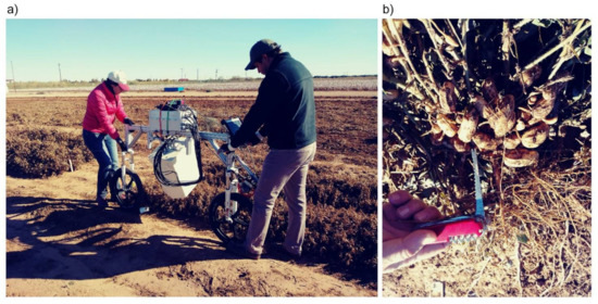
Figure 1.
The peanut trial was scanned with an air-launched multichannel GPR antenna array while aboveground biomass was present (a). Peanut pods located just beneath the surface and above the root of the plant (b).
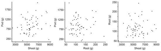
Figure 2.
Biomass data are provided per plot, and includes shoot, pod, and root biomass, with no statistically significant correlation between these three physical attributes.
The GPR system used in this study was developed by IDS GeoRadar and comprises an array of four pairs of downward-looking vee-dipole-type antennae functioning as an air-launched multichannel configuration with central frequency 1.8 GHz. The system was initially developed for landmine detection [26,30,31]. Because agricultural soil surface is typically soft and uneven and aboveground biomass is often present, the air-launched deployment of the antenna array was deemed appropriate for this application. An air-launched antenna, however, introduces a strong ground-surface return that must be taken into account. The antenna array was mounted on a bicycle-style cart and tilted at an angle towards the plants with the linear array of transmit-receive antennae oriented perpendicular to the direction of scanning. We moved the cart with the GPR instrument over the uncultivated area outside the edge of each plot (Figure 1). For this study, GPR data were acquired in seven channels, but three of the channels contained excessive noise and were excluded from the analysis.
Figure 3 demonstrates common GPR terminology and a brief description follows. The returned signal from a single outgoing GPR pulse on a given antenna is referred to as an ‘A-scan’ or a ‘trace’. ‘Time window’ is a GPR acquisition parameter that is user-specified. In this study we used an 18 ns time window, meaning that a transmit antenna sent an electromagnetic pulse at time zero and a receive antenna recorded the voltage of the returned electromagnetic signal during the subsequent 18 ns. Within the 18 ns window, the receiver recorded 512 observations, termed ‘samples’, meaning that each trace contains 512 samples taken at 0.035 ns time intervals. The time window refers to two-way travel time since the signal must travel from the transmit antenna, through the subsurface, and then back to the receive antenna. The GPR antenna array was moved along a row of plants and traces were acquired at 1 cm intervals, as measured by an encoder wheel. Since we used a multichannel system, multiple transmit–receive antenna pairs were used thus collecting data simultaneously at multiple channels. For each channel, the traces collected along a row are assembled to form a 2D representation of the GPR data, called a B-scan, which in essence is an image of a vertical section of the subsurface. Each column in a B-scan corresponds to a single trace, while each row in the image consists of the samples collected at the same time for each trace. Due to the geometry of the multichannel antenna array used in this study, the GPR data are acquired in the form of a swath. A swath consisting of multiple channels may be assembled to form a 3D GPR data cube, with a GPR data cube being referred to as a C-scan.
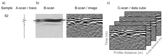
Figure 3.
In GPR terminology, (a) a single GPR observation is referred to as a ‘sample’ and the samples collected from a single channel are referred to as an A-scan or a trace; (b) a collection of A-scans along an acquisition line is referred to as a B-scan and is often visualized as an image; and (c) when multiple channels are used, the resulting collection of B-scans is referred to as a C-scan.
The GPR system is equipped with the capability to manually place digital markers in the data, used to mark the start and end of peanut plots along an acquisition line while scanning. To ensure that analysis is not affected by the unequal length of agricultural plots, we cropped the GPR B-scans into equal sections of 3 m (9.84 feet) in length. Figure 4 shows 10 such sections extracted from channel-3 data with the corresponding peanut yield (g) displayed above in red. Portions of B-scans that contain peanut information are often distinguished visually; for example, at 20 m from the start of the B-scan in Figure 4 is a gap between two sections, and one can observe a different density of hyperbolas to the right and to the left of the gap. We used this type of visual information to separate the sections manually and ensure that they are of equal length. Further analysis should be undertaken to assess the effects of cropping the B-scans to make them of equal length as compared to using the original variable-length B-scans as marked in the field.
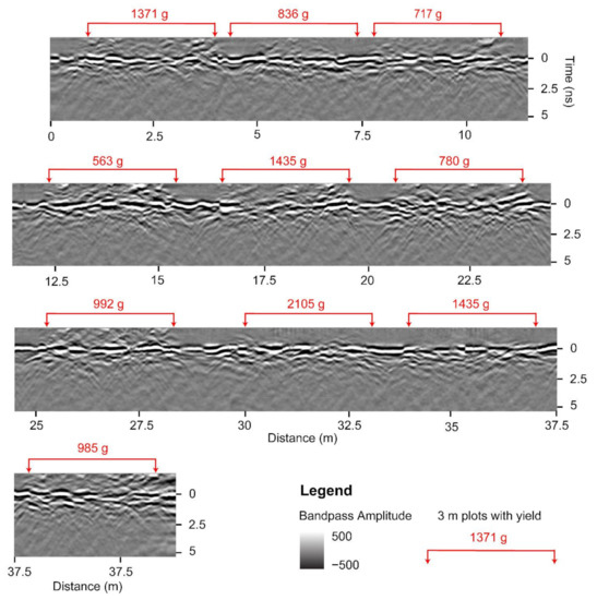
Figure 4.
A radargram of a single acquisition line processed up to bandpass filter for channel-3 demonstrating the location of ten 3 m peanut plots. Values in red are the corresponding plot-level peanut yield.
2.2. GPR Data Processing
GPR data processing and analysis was performed using GPR-Studio version 1.0.1 (Crop Phenomics LLC, College Station, TX, USA, [32]). Borrowing terminology from remote sensing, we define a subset to be a portion of a larger image. Figure 5 shows GPR subsets for two of the agricultural plots: plot 247, which contains the least biomass of the trial (162.9 g) and plot 263, which contains the largest biomass of the trial (2105.3 g). Each plot was scanned twice by the GPR system, with individual passes going over one row of plants. Since the trial consisted of two-row plots, the two GPR passes scanned different peanut plants. For the analysis, the two 3-m-long passes were combined and thus a combined subset is a total length of 6 m. Figure 5 shows GPR data for the four active channels. We performed preliminary analysis using only single-channel data, but the correlations to biomass were stronger when data from all four channels were analyzed together. Data from channels 1, 2, and 7 were not processed as they contained excessive noise that we were unable to remove.
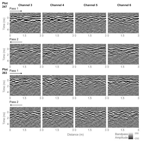
Figure 5.
Radargrams processed up to bandpass filter for all four channels and two of the plots. The two passes over the plots are indicated with arrows. Plot 247 contains the least biomass of the trial (162.9 g) and plot 263 contains the largest biomass of the trial (2105.3 g).
Since the antenna array was tilted when the scans were performed, and there is a fixed distance between each of the antennas in the array, data as collected are not vertically aligned between channels, which means that the peanut-pod information appears at different times in equivalent traces on different channels. To account for these differences, we visually identified the vertical location of the surface return on each B-scan and time-shifted the data in that channel to a common temporal datum. For the remainder of the analysis, we established the common datum to 0 ns, which separates samples above the surface as being recorded at negative time and samples below the surface as positive time. This was done so the data presentation resembles how a single ground-coupled antenna would return the GPR signal, thereby assisting with the interpretation of the GPR data. A total of 200 time samples from each trace were used, including 50 samples above the surface and 150 samples below. In our GPR data, the surface can be recognized due to the strong ground clutter, and insofar as possible we assigned the middle of the ground-clutter interval to be time zero.
GPR data processing was performed to mitigate noise, focus the signal, and convert the focused signal to positive values. The workflow included background correction, bandpass filter, Kirchoff migration, and Hilbert transform (Figure 6 and Figure 7). As demonstrated in Figure 6, the raw B-scans contain horizontal stripes that are removed with a background correction. A bandpass filter removes low and high frequency signal energy. Different bandpass filter ranges were tested; a 0.1–2.4 GHz range gave best results. Migration focused the signal while the Hilbert transform converted the signal to positive values. A different workflow, or the same workflow based on different processing parameters, may produce similar or better results and should be further investigated. Following the GPR data processing, the B-scans were subset to plot level. The two passes over each peanut plot were combined to form the final analysis plots of 6 m each, and percentile thresholding was performed (details below) to extract plot-level GPR features. The latter were then correlated to peanut pod biomass (Figure 8). The entire workflow was performed within GPR Studio—a combination of graphical user interface software and a Python library that provide GPR processing, analysis, and visualization capabilities.
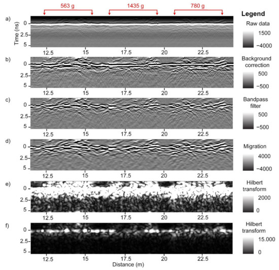
Figure 6.
Radargrams of GPR processing: raw GPR data (a), background correction (b), bandpass filter (c), Kirchoff migration (d), and Hilbert transform (e,f). The surface is indicated as time 0 ns. The same Hilbert transform radargram is displayed twice with two different image enhancement methods to highlight different features. Values in red are the corresponding plot-level peanut yield values for the three plots included in these radargrams.
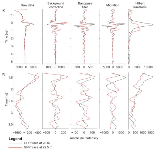
Figure 7.
A-scans of GPR processing demonstrating background correction, bandpass filter, Kirchoff migration and Hilbert transform. These A-scans are at 20 and 22.5 m from the data displayed in Figure 6. The upper panel displays the A scans for the full depth of analyzed (a), and the lower panel displays the data zoomed in to a smaller depth range that also includes the depth where the highest correlations are observed (b).
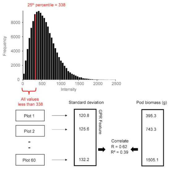
Figure 8.
GPR feature extraction example is demonstrated. The histogram displays the GPR data for all plots combined for a specific analysis window. The red line shows the 25th percentile for these data, which is 338. The GPR feature is computed for data below the threshold, which in this case is all values less than 338. For each plot, only the values that fall within this range are considered in the analysis. The standard deviation of these values and other summary statistics are calculated. The GPR features thus extracted are then correlated to plot-level peanut pod biomass.
Similar processing and analysis were performed in previous studies of GPR applications to cassava tubers [23,24], fine roots [22], and tree roots, e.g., [15], but a definite methodology is not yet standardized. In this study, we performed systematic image thresholding analysis, wherein different threshold ranges, analysis window sizes, and summaries were performed on GPR data values above and below the percentile threshold. The following four summary statistics were used: mean, standard deviation, sum, and number of nonzero values (counts).
2.3. Thresholding Analysis
Analysis was performed within a sliding window that is moved down a B-scan one sample at a time (i.e., one row at a time if the radargram is viewed as an image). The concept of an analysis window is demonstrated in Figure 9. The analysis window includes only those samples that fall within the window and it also includes all of the GPR traces within a plot-level C-scan. The size of the window was varied; the following window sizes were utilized: 1, 2, 3, 4, 5, 7, 10, 15, 20, and 25 samples. The conversions of the time-window size from number of samples first to two-way travel time and then to depth for three different soil dielectric properties is presented in Table 2. Three soil moisture cores were collected in the field, and moisture was converted to soil dielectric permittivity, yielding an average value ε ~ 6.6, which corresponds to signal velocity of ~0.12 m/ns. However, it is always problematic to use this or any other particular value for the time-to-depth conversion because of the strong heterogeneity of subsurface dielectric permittivity. Therefore, in this study we report results in terms of two-way travel time instead of depth.
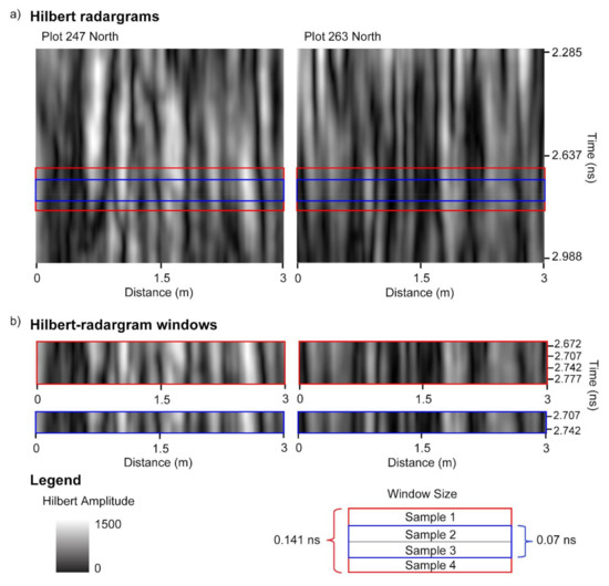
Figure 9.
Hilbert transform of GPR data for one of the passes of plots 247 and 263 (a). Plot 247 contains the least biomass of the trial (162.9 g) and plot 263 contains the largest biomass of the trial (2105.3 g); these plots are also displayed in Figure 5. Two window sizes are demonstrated (b)—window size of 2 samples (0.07 ns) and window size of 4 samples (0.141 ns). The vertical locations of the two windows as indicated by the sample closest to the surface are at 2.672 and 2.707 ns.
Table 2.
Conversion of two-way travel time to depth for the ten window sizes used in this study. This conversion is performed using three dielectric constants (ε) corresponding to three different velocities (v).
For each agricultural trial plot, the GPR Hilbert amplitudes contained within the analysis window were combined and a percentile value was calculated. The raw GPR data are the recorded voltages of the returned electromagnetic signals, whereas the GPR data used in the thresholding analysis are the Hilbert-transformed amplitudes (Figure 6 and Figure 7). Note that the Hilbert amplitude scale is somewhat arbitrary. The concept of percentile is demonstrated in Figure 8. The figure shows an example wherein the GPR feature is the standard deviation of Hilbert amplitudes below the 25th percentile. The 25th percentile is the value below which 25% of the amplitudes reside; in this example it is 338. This means that amplitude values less than 338 comprise 25% of the dataset, while higher values comprise the remaining 75%. This study used the following percentile thresholds: 3, 5, 10, 15, 25, 30, 35, 40, 45, 50, 55, 60, 65, 70, 75, 85, 90, 95, and 97.
Summary statistics for each plot were formed by calculating the mean, standard deviation, sum, and number of nonzero values (counts) of the Hilbert amplitudes that fall above or below each of the percentile thresholds. These statistics, termed ‘GPR features’ were then correlated to the field-observed biomass of the peanut pods. The latter is a conventional measure of peanut yield. We performed simple linear regressions between individual GPR features and peanut pod biomass, and multiple linear regression between a particular set of GPR features and peanut pod biomass. Specifically, we chose the best performing GPR features as indicated by their correlation to peanut yield to use in the multiple linear regression. Estimated and measured yields were then correlated to evaluate the model’s performance in estimating the actual yield. Results are reported in terms of percent explained variability, i.e., the coefficient of determination R2 multiplied by 100. The coefficient of determination is the square of the Pearson correlation coefficient R.
3. Results
Our results indicate that thresholding analysis produces strong correlations between individual GPR features and peanut yield, while multiple linear regressions between a set of GPR features and peanut yield improve the results. Correlations were found to be sensitive to changes in the analysis parameters and depended on peanut type. This research demonstrates that thresholding analysis is an appropriate method for extracting GPR information that is diagnostic of peanut yield.
3.1. Regression Analysis
To best characterize the GPR information related to peanut yield, we determined the time window within the Hilbert-transformed radargram that contains the most information about the peanut pods. Specifically, we sought the set of data-partition parameters that generated the strongest correlation between individual GPR features and peanut yield (Table 3 and Figure 10).
Table 3.
Strongest correlations for the full data set of 60 plots and for the data below the specified percentile threshold. Correlations are significant at p < 0.05.
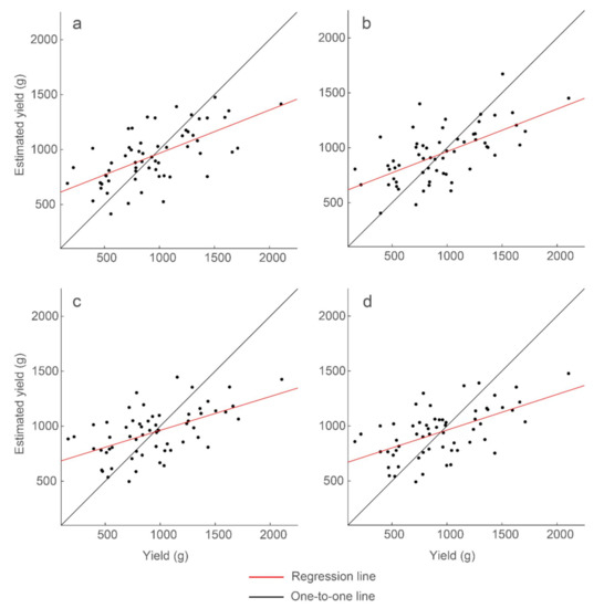
Figure 10.
Strongest correlations of the simple linear regression models between individual GPR features and yield. The GPR features are (a) mean with R2 = 0.39, (b) standard deviation with R2 = 0.39, (c) sum with R2 = 0.31, and (d) count with R2 = 0.32. Model results and parameters are presented in Table 3.
Mean and standard deviation as GPR features produced the strongest correlations with peanut-pod biomass, achieving 39% explained variability. Sum of the Hilbert-transform amplitudes within a threshold range and counts of the nonzero values of the Hilbert-transform amplitudes within a threshold range produced similar, but lower, correlations with 31% and 32% explained variability, respectively. These correlations were derived from GPR amplitudes within the same narrow time windows. The best-performing threshold percentiles, however, differed for the different features: 25th and 35th percentiles for mean, 50th percentile for standard deviation, and 3rd and 5th percentiles for sum and count. These features are for data below the percentile threshold. The results show that there is a specific time window within a radargram wherein maximal information about peanut yield is contained, although there are different ways to partition and summarize the GPR data to achieve a strong correlation.
3.2. Multiple Linear Regression Analysis
The GPR features that correlated strongest with peanut yield were combined to form a multiple linear regression model. To select the features to be included in the final predictive model, we tested different combinations of features, including interactions between pairs of features (an interaction term is the product of two variables). We also investigated overlaps of information between pairs of features (Table 4) to assess in which cases combining features would be meaningful. There are five GPR features presented in Table 3, but as indicated by Table 4, the features based on sum and pixel count are correlated, such that they provide essentially redundant information. Therefore, we chose only one of these two, sum. In the end, only three GPR features are considered: mean, standard deviation, and sum. We tested all possible combinations of these three features and their interaction terms. The multiple regression model with the strongest prediction capability achieved 51% explained variability (Table 5 and Figure 11) for all peanut market types. Higher explained variabilities were found after the dataset was partitioned by peanut type. The Spanish type, for instance, recorded 95% explained variability.
Table 4.
Percent explained variability (R2 * 100) between GPR features and yield, and between pairs of GPR features. These are the six GPR features presented in Table 3.
Table 5.
Multiple linear regression results for the full data set and for data per peanut type. Scan location refers to two-way travel time. Window size is reported in number of samples and in ns, as used in Table 2.
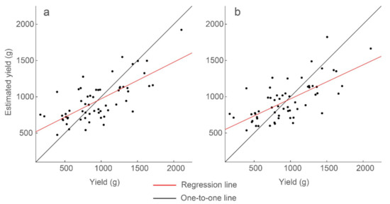
Figure 11.
Strongest correlations of the multiple regression models for the full data set of 60 plots. Presented are (a) the model with variable analysis parameters and R2 = 0.51, and (b) the model with constant analysis parameters and R2 = 0.47. Model results and parameters are presented in Table 5.
The final multiple regression model includes the three GPR features and their bivariate interaction terms:
where is the standard deviation feature at the 50th percentile, is the mean at the 35th percentile, and is the sum at the 3rd percentile for the values below the percentile threshold. All features are normalized to the (0,1) interval. Normalizing the GPR features does not change the estimated yield but generates regression coefficients that are easier to interpret. The equation above represents the strongest correlation model we found between GPR data and peanut yield but carries the limitation that the three GPR features were based on different threshold parameters.
To evaluate effect of this limitation, GPR features generated using a single thresholding percentile were combined into a multiple linear regression model. The free parameters are scan depth, thresholding range, and window size. We found the parameters that generated the optimal standard deviation feature: scan location 2.67 ns below the surface, window size 0.141 ns, 50th percentile, and for the data below the threshold. Using mean, standard deviation, and sum, and their interaction terms, we generated a multiple regression model with 47% explained variability (Table 5 and Figure 11):
It is important to reduce the number of parameters so as to more efficiently optimize or calibrate the GPR analysis when the technology is put into production. It is promising that only 4% less variability is achieved when using features generated with the same thresholding analysis parameters, as compared to using the same features with variable parameters.
The correlations derived are stronger if regression models are constructed separately for each peanut type. Using the same set of thresholding and regression model parameters that generated the 47% explained variability for the full data set, we constructed a regression model for each peanut type. We also created regression models wherein thresholding analysis parameters were allowed to vary for each peanut type. When investigating at a ‘depth’ of 2.67 ns (the same depth used for the full data set), Spanish peanut exhibited the strongest correlation, with up to 95% explained variability, followed by Valencia and Virginia with up to 76% and 68% explained variability, respectively (Table 5 and Figure 12). Analysis of runners, which are the most popular peanut market type, underperformed with 40% explained variability, but this value increased to 77% explained variability at a lower depth (3.59 ns). These results show the higher predictive capability of regression models constructed for specific peanut types with the limitation being the small sample size for these models (Table 1).
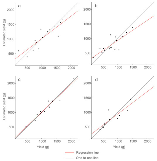
Figure 12.
Strongest correlations of the multiple regression models for each peanut market type. Presented are (a) the model for runners and R2 = 0.77, (b) the model for Virginia and R2 = 0.68, (c) the model for Spanish and R2 = 0.95, and (d) the model for Valencia and R2 = 0.76. Model results and parameters are presented in Table 5.
3.3. Mean and Standard Deviation
Using mean and standard deviation as features generated the strongest single linear regression models, with mean exhibiting a negative relationship and standard deviation exhibiting a positive relationship to yield. Figure 13 demonstrates several correlation peaks where these two GPR features exhibit opposite relationships to yield. To further examine these trends, five agricultural plots that lie on or close to the regression line (Figure 10) were selected. Figure 14 displays histograms of the Hilbert amplitudes associated with each plot, with biomass increasing from left to right. The negative relationship between mean and standard deviation is apparent: as the mean (of the blue subset) decreases it moves to the left of the histogram, while the standard deviation (of the blue subset) increases. Portions of the Hilbert-transform radargrams representing the two plots containing the least and the most biomass are displayed in Figure 9. The plot with the least biomass exhibits several large regions of high Hilbert-amplitude intensity indicating greater homogeneity, while the plot with the most biomass displays smaller regions of alternating high and low intensity, thus exhibiting higher variability.
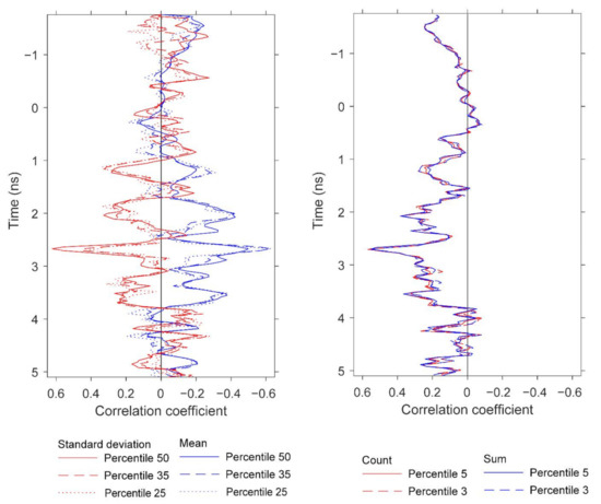
Figure 13.
Correlations at depth between pod biomass (yield) and the GPR features presented in Table 3. The figure displays the depths at which strong correlations for peanut yield are observed and compares the correlations for the GPR features based on different percentiles for standard deviation, mean, count, and sum.
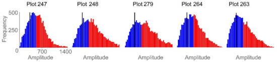
Figure 14.
Histograms of plot-level GPR data for five agricultural plots. Red bars indicate data above the 50th percentile threshold and blue bars indicate data below that threshold. The black vertical line is the mean of the data below the percentile threshold. The five histograms are displayed with the same frequency and amplitude range. For the five agriculture plots and from left to right, peanut yield ranges from low to high, mean ranges from high to low, and standard deviation ranges from low to high.
3.4. Count
The correlations calculated per plot for GPR features above the percentile threshold did not correlate strongly (Table 6). The count feature generated correlations of the same strength, but opposite sign from the correlation below the percentile threshold. This was expected because simply switching the percentile method preserves the same variability in the count. Counting nonzero values below the 3rd (5th) percentiles and counting nonzero values above the 3rd (5th) percentiles generated correlations of R = 0.57 (−0.57) respectively, for 32% explained variability (i.e., R2 = 0.32).
Table 6.
Strongest correlations for the full data set of 60 plots and for the data above the specified percentile threshold. Correlations are significant at p < 0.05.
3.5. Root and Shoot Biomass
We observed significant correlations between GPR features and both root and aboveground (shoot) biomass. It was not within the scope of this study to treat separately these two peanut attributes, but herein we report preliminary results for potential future development. The results do provide further information about the peanut yield information content in GPR scans. Similar to Figure 13, Figure 15 and Figure 16 display pairwise correlations for peanut physical attributes and GPR features as a function of time (proxy for depth). The correlations for root and shoot biomass contrast to those found earlier for pod biomass (i.e., yield) with respect to the sign of the relationships. The correlations for root and shoot oscillate with depth; for example, the root correlation peak at 3.1 ns exhibits a positive relation for mean and a negative relation for standard deviation, while the correlation peak at 4.2 ns exhibits a negative relation for mean and a positive relation for standard deviation. With respect to depth, some of the correlation peaks for the three attributes are ordered as expected from the basic plant architecture. For example, while correlation peaks for all three attributes occur in the depth range of 2.3–3.1 ns, the peak for shoot is at 2.3 ns, the peak for pod is at 2.7 ns, and the peak for root is at 3.1 ns. More conclusive results would be obtained by carefully optimizing the GPR analysis for root and shoot biomass separately.
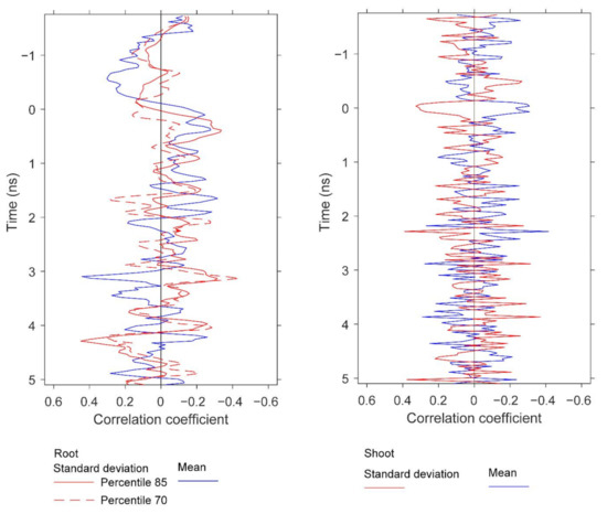
Figure 15.
Correlations at depth between root biomass and the GPR features, and between shoot biomass and GPR features. The figure compares the depths at which strong correlations for root and shoot biomass are observed. The GPR features are based on standard deviation and mean. Specifically, the results for root biomass are generated using window size 3, and the percentiles are 85th and 70th for standard deviation and 25th for mean. The results for shoot are generated using window size 1 and the percentiles are 25th for standard deviation and 10th for mean. All of these results are for data below the specified percentile threshold.
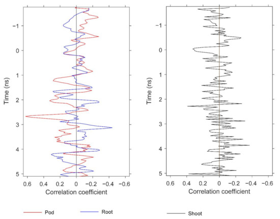
Figure 16.
Correlations at depth between biomass and GPR features. The figure compares the depths at which strong correlations for pod, root, and shoot biomass are observed. The GPR features are based on standard deviation.
4. Discussion
GPR technology has the potential for rapid, relatively inexpensive, and nondestructive peanut yield monitoring. The present study is the first to demonstrate consistent correlations between GPR data and peanut yield. Up to 51% explained variability is achieved by using multiple GPR features with parameters optimized for each feature. Up to 47% explained variability is achieved by using GPR features generated with a single set of parameters (Table 5 and Figure 11). These results demonstrate that GPR technology detects peanut yield, and that thresholding analysis extracts GPR information correlating strongly to peanut yield. The correlations may be sufficiently high to use the technology as a selection tool in breeding trials; however, the results must be improved and replicated at larger scales before the technology is developed for reliable commercial yield monitoring. Our results demonstrate stronger correlations when regression models are developed for specific peanut market types (Table 5 and Figure 12), but the results must be interpreted with caution because of the small sample sizes (Table 1). Once the results are confirmed with larger datasets, we may achieve correlations appropriate for reliable commercialization, thus adding new sensors and capabilities to the growing set of digital agriculture technologies.
Developing GPR technology for noninvasive peanut yield assessment requires standardizing the analysis parameters. The radar-inferred depth at which peanuts are detected is one of these parameters. A key observation is that the information about peanut yield is contained only within a narrow depth range (Table 2, Table 3, and Table 5) but the correlations also oscillate with respect to depth (Figure 13, Figure 15, and Figure 16). In previous research, we observed a similarly narrow depth range for other root systems and analysis methods. An implication of this finding is that analysis to extract GPR features should be performed only on the depth range wherein the maximum information about peanut yield is located. Another implication is that channels must be temporally aligned at the surface; otherwise, different channels would contain peanut yield information at different depths. Repeating the analysis at different agricultural sites would help determine how depth as an analysis parameter could become standardized.
The complex travel path of the GPR signal must also be considered. It is problematic to use an estimate of soil dielectric from an in situ probe as the basis for a time-to-depth conversion. Using probe-derived soil dielectric 6.628 results in depths of 15.5 and 20.8 cm for two-way travel times of 2.67 and 3.59 ns, respectively, while peanut pods are expected to be found within ~5 cm below the surface. We posit multiple interactions between GPR signal and peanut pods because peanut pods are composite objects (Figure 1). In addition, each pod contains both a shell and a kernel, adding to the media interfaces with which the propagating electromagnetic wave interacts. For example, runners are detected lower in the radargram than other peanut types, suggesting a more complex travel path. As runners is the most popular peanut type, this discovery should be investigated further.
Other analysis parameters beside depth are the thresholding range and the choice of data summary statistics. With respect to threshold range, we determined that summarizing the data below different percentile thresholds generated the strongest correlations for all GPR features except count. Count is a unique feature insofar as it derives the same correlation strength but opposite sign depending on whether data below or above the threshold is used. We also found negative correlations to yield that are meaningful; an example being the mean feature. Negative correlations between GPR signal attributes and root biomass were reported by [22] but not investigated in detail. We posit that greater subsurface variability, especially in the presence of small composite objects, may cause greater signal attenuation and thus the lower mean of the signal as compared to a subsurface with less variability. We also found that while some GPR feature pairs such as sum and count are strongly correlated, other pairs are not; therefore, combining only uncorrelated features in multiple regression models improved the correlations to yield.
Our work builds on the knowledge of other studies that have used GPR to measure belowground tree and crop traits. The authors of [24] utilized an upper threshold of 80 for GPR data scaled on [0,256] using count as the feature. The threshold was determined by calculating the average of known locations of cassava roots in a radargram. The authors of [22] tested thresholds based on several GPR features but in the end derived correlations that were not based on threshold. Our research shows that a systematic search of the optimal thresholding range is necessary for successful application of GPR root-trait analysis, and that various kinds of summary statistics should be considered. In this respect, this work fits within the broader literature related to model optimization, e.g., [33].
An important discussion in the GPR literature concerns the effect of soil and root moisture variability on the GPR signal [22,34]. Specifically, a GPR signal contains information about subsurface variability, including information that is unrelated to the belowground trait that we aim to estimate. Deconvolving the unwanted from the wanted signal is critical to building the correlations needed to operationalize the technology. Our results suggest that by performing thresholding such that the high-amplitude signal is removed, we may also be reducing the effects of pod moisture variability on the GPR signal. This is because a high-amplitude signal is generated at the interface of two media with strongly contrasting dielectric properties. The latter are determined largely by moisture content. With respect to soil moisture variability, peanut forms dense clusters of pods close to the surface (within ~5 cm below the surface) and the strongest correlations with yield are extracted from a narrow depth range. Thus, the signal may consist of only small amounts of information about soil variability as compared to other GPR applications for which the crop trait of interest is lower in the subsurface. Alternatively, pod and soil moisture variability may be the reason why we can explain only half of the pod biomass variability. An implication of this is that deconvolution techniques to separate soil and pod moisture signal from pod biomass signal may be necessary, for which spectral analysis may be an appropriate approach.
This work contributes to developing the theory and methodology necessary for applying GPR technology to measure peanut yield. Developing GPR technology for yield monitoring requires that we find optimal correlations between GPR signal and yield and develop excellent predictive models. We derived correlations of up to 95% explained variability (Table 5 and Figure 12) with a multiple regression model developed for a specific peanut market type; however, a larger dataset is necessary to confirm its reliability. With respect to standardizing the analysis parameters, we must perform studies across diverse sites with different soil characteristics. We may find that some field calibration is necessary and model parameters may have to be set according to specific site characteristics. A larger dataset is also necessary to perform model validation, i.e., testing of data that were not used during model development. Most importantly, a larger data set from multiple sites would allow utilization of deep learning techniques for creating general yield-predictive models.
The results of this study build on the existing knowledge of GPR in agriculture by developing a standardized method for optimal thresholding-parameter search. This method is coded in Python and available in the software package GPR-Studio [32], which contains methods to perform GPR data processing and methods for agricultural analysis of GPR data. We expect that GPR technology will become a phenotyping tool for peanut breeders, as well as a commercial yield-monitoring system for peanut farmers and industry, and this study contributes to this vision.
5. Conclusions
Achieving up to 51% explained variability for the 60-plot dataset demonstrated that we can extract peanut yield information through GPR technology and thresholding analysis. At the same time, achieving up to 95% explained variability with a predictive model constructed for a particular peanut market type shows sufficient promise for deploying this technology within a digital agriculture framework, with a stipulation being that the results must first be confirmed on larger datasets. The present work is significant in presenting a new methodology for performing a systematic search for optimal thresholding parameters, which has not been demonstrated before within the emerging field of GPR in agriculture. This work advances developing GPR technology for nondestructive, large-scale peanut phenotyping and yield monitoring, with applicability to other crops.
Author Contributions
Conceptualization, I.D.D., H.A.R.-G., I.B.-P., B.L.T., M.E.E. and D.B.H.; data acquisition, I.D.D., H.A.R.-G., I.B.-P., B.L.T., M.D.B., P.P. and D.B.H.; software, I.D.D. and H.A.R.-G.; analysis, I.D.D.; writing—original draft preparation, I.D.D.; writing—review and editing, I.D.D., I.B.-P., T.A., M.E.E., M.D.B. and D.B.H.; funding acquisition, D.B.H. All authors have read and agreed to the published version of the manuscript.
Funding
This work was supported with grants from the National Science Foundation award number 1543957—BREAD PHENO: High Throughput Phenotyping Early Stage Root Bulking in Cassava using Ground Penetrating Radar to Dirk B. Hays, and by the Department of Energy of the United States (ARPA-E Award, No. DE-AR0000662)—Development of ground penetrating radar for enhanced root phenotyping and carbon sequestration also to Dirk B. Hays.
Institutional Review Board Statement
Not applicable.
Informed Consent Statement
Not applicable.
Data Availability Statement
The data presented in this study are available on request from the corresponding author. The data are not publicly available due to product commercialization.
Acknowledgments
The authors would like to thank Melonie White of the USDA-ARS Cropping Systems Research Laboratory for technical assistance with physiological measurements of peanut field plots.
Conflicts of Interest
The authors declare no conflict of interest.
References
- Variath, M.T.; Janila, P. Economic and academic importance of peanut. In The Peanut Genome; Springer: Berlin/Heidelberg, Germany, 2017; pp. 7–26. [Google Scholar]
- Colvin, B.; Rowland, D.; Ferrell, J.; Faircloth, W. Development of a Digital Analysis System to Evaluate Peanut Maturity. Peanut Sci. 2014, 41. [Google Scholar] [CrossRef]
- Durrence, J.; Hamrita, T.; Vellidis, G. A Load Cell Based Yield Monitor for Peanut Feasibility Study. Precis. Agric. 1999, 1, 301–317. [Google Scholar] [CrossRef]
- Kirk, K.R.; Han, Y.J.; Porter, W.M.; Monfort, W.S.; Henderson, W.G.; Thomas, J. Development of a Yield Monitor for Peanut Research Plots; American Society of Agricultural and Biological Engineers: St. Joseph, MI, USA, 2012; p. 1. [Google Scholar]
- Porter, W.; Ward, J.; Taylor, R.; Godsey, C. A Note on the Application of an AgLeader® Cotton Yield Monitor for Measuring Peanut Yield: An Investigation in Two US States. Peanut Sci. 2020, 47, 115–122. [Google Scholar] [CrossRef]
- Colvin, B.C.; Tseng, Y.-C.; Tillman, B.L.; Rowland, D.L.; Erickson, J.E.; Culbreath, A.K.; Ferrell, J.A. Consideration of Peg Strength and Disease Severity in the Decision to Harvest Peanut in Southeastern USA. J. Crop Improv. 2018, 32, 287–304. [Google Scholar] [CrossRef]
- Anco, D.J.; Thomas, J.S.; Jordan, D.L.; Shew, B.B.; Monfort, W.S.; Mehl, H.L.; Small, I.M.; Wright, D.L.; Tillman, B.L.; Dufault, N.S. Peanut Yield Loss in the Presence of Defoliation Caused by Late or Early Leaf Spot. Plant Dis. 2020, 104, 1390–1399. [Google Scholar] [CrossRef]
- Meister, R.; Rajani, M.; Ruzicka, D.; Schachtman, D.P. Challenges of Modifying Root Traits in Crops for Agriculture. Trends Plant Sci. 2014, 19, 779–788. [Google Scholar] [CrossRef]
- Atkinson, J.A.; Pound, M.P.; Bennett, M.J.; Wells, D.M. Uncovering the Hidden Half of Plants Using New Advances in Root Phenotyping. Curr. Opin. Biotechnol. 2019, 55, 1–8. [Google Scholar] [CrossRef]
- Wasson, A.P.; Nagel, K.A.; Tracy, S.; Watt, M. Beyond Digging: Noninvasive Root and Rhizosphere Phenotyping. Trends Plant Sci. 2020, 25, 119–120. [Google Scholar] [CrossRef] [PubMed]
- Pflugfelder, D.; Metzner, R.; van Dusschoten, D.; Reichel, R.; Jahnke, S.; Koller, R. Non-Invasive Imaging of Plant Roots in Different Soils Using Magnetic Resonance Imaging (MRI). Plant Methods 2017, 13, 102. [Google Scholar] [CrossRef] [PubMed]
- Teramoto, S.; Takayasu, S.; Kitomi, Y.; Arai-Sanoh, Y.; Tanabata, T.; Uga, Y. High-Throughput Three-Dimensional Visualization of Root System Architecture of Rice Using X-ray Computed Tomography. Plant Methods 2020, 16, 66. [Google Scholar] [CrossRef]
- Středa, T.; Haberle, J.; Klimešová, J.; Klimek-Kopyra, A.; Středová, H.; Bodner, G.; Chloupek, O. Field Phenotyping of Plant Roots by Electrical Capacitance—A Standardized Methodological Protocol for Application in Plant Breeding: A Review. Int. Agrophys. 2020, 34, 173–184. [Google Scholar] [CrossRef]
- Corona-Lopez, D.D.; Sommer, S.; Rolfe, S.A.; Podd, F.; Grieve, B.D. Electrical Impedance Tomography as a Tool for Phenotyping Plant Roots. Plant Methods 2019, 15, 49. [Google Scholar] [CrossRef]
- Butnor, J.R.; Doolittle, J.; Johnsen, K.H.; Samuelson, L.; Stokes, T.; Kress, L. Utility of Ground-penetrating Radar as a Root Biomass Survey Tool in Forest Systems. Soil Sci. Soc. Am. J. 2003, 67, 1607–1615. [Google Scholar] [CrossRef]
- Stover, D.B.; Day, F.P.; Butnor, J.R.; Drake, B.G. Effect of Elevated CO2 on Coarse-root Biomass in Florida Scrub Detected by Ground-penetrating Radar. Ecology 2007, 88, 1328–1334. [Google Scholar] [CrossRef]
- Hirano, Y.; Dannoura, M.; Aono, K.; Igarashi, T.; Ishii, M.; Yamase, K.; Makita, N.; Kanazawa, Y. Limiting Factors in the Detection of Tree Roots Using Ground-Penetrating Radar. Plant Soil 2009, 319, 15–24. [Google Scholar] [CrossRef]
- Cui, X.; Chen, J.; Shen, J.; Cao, X.; Chen, X.; Zhu, X. Modeling Tree Root Diameter and Biomass by Ground-Penetrating Radar. Sci. China Earth Sci. 2011, 54, 711–719. [Google Scholar] [CrossRef]
- Borden, K.A.; Isaac, M.E.; Thevathasan, N.V.; Gordon, A.M.; Thomas, S.C. Estimating Coarse Root Biomass with Ground Penetrating Radar in a Tree-Based Intercropping System. Agrofor. Syst. 2014, 88, 657–669. [Google Scholar] [CrossRef]
- Grote, K.; Anger, C.; Kelly, B.; Hubbard, S.; Rubin, Y. Characterization of Soil Water Content Variability and Soil Texture Using GPR Groundwave Techniques. J. Environ. Eng. Geophys. 2010, 15, 93–110. [Google Scholar] [CrossRef]
- Wu, K.; Rodriguez, G.A.; Zajc, M.; Jacquemin, E.; Clément, M.; De Coster, A.; Lambot, S. A New Drone-Borne GPR for Soil Moisture Mapping. Remote Sens. Environ. 2019, 235, 111456. [Google Scholar] [CrossRef]
- Liu, X.; Dong, X.; Xue, Q.; Leskovar, D.I.; Jifon, J.; Butnor, J.R.; Marek, T. Ground Penetrating Radar (GPR) Detects Fine Roots of Agricultural Crops in the Field. Plant Soil 2018, 423, 517–531. [Google Scholar] [CrossRef]
- Delgado, A.; Novo, A.; Hays, D.B. Data Acquisition Methodologies Utilizing Ground Penetrating Radar for Cassava (Manihot Esculenta Crantz) Root Architecture. Geosciences 2019, 9, 171. [Google Scholar] [CrossRef]
- Delgado, A.; Hays, D.B.; Bruton, R.K.; Ceballos, H.; Novo, A.; Boi, E.; Selvaraj, M.G. Ground Penetrating Radar: A Case Study for Estimating Root Bulking Rate in Cassava (Manihot Esculenta Crantz). Plant Methods 2017, 13, 65. [Google Scholar] [CrossRef] [PubMed]
- Shen, X.; Foster, T.; Baldi, H.; Dobreva, I.; Burson, B.; Hays, D.; Tabien, R.; Jessup, R. Quantification of Soil Organic Carbon in Biochar-Amended Soil Using Ground Penetrating Radar (GPR). Remote Sens. 2019, 11, 2874. [Google Scholar] [CrossRef]
- Nuzzo, L.; Alli, G.; Guidi, R.; Cortesi, N.; Sarri, A.; Manacorda, G. A New Densely-Sampled Ground Penetrating Radar Array for Landmine Detection; IEEE: New York, NY, USA, 2014; pp. 969–974. [Google Scholar]
- García-Fernández, M.; López, Y.Á.; Andrés, F.L.-H. Airborne Multi-Channel Ground Penetrating Radar for Improvised Explosive Devices and Landmine Detection. IEEE Access 2020, 8, 165927–165943. [Google Scholar] [CrossRef]
- Everett, M.E. Near-Surface Applied Geophysics; Cambridge University Press: Cambridge, UK, 2013; ISBN 1-107-01877-3. [Google Scholar]
- Annan, A. Electromagnetic Principles of Ground Penetrating Radar; Elsevier: Amsterdam, The Netherlands, 2009; Volume 1. [Google Scholar]
- Montoya, T.P.; Smith, G.S. Vee Dipoles with Resistive Loading for Short-pulse Ground-penetrating Radar. Microw. Opt. Technol. Lett. 1996, 13, 132–137. [Google Scholar] [CrossRef]
- Kim, K.; Scott, W.R. Design of a Resistively Loaded Vee Dipole for Ultrawide-Band Ground-Penetrating Radar Applications. IEEE Trans. Antennas Propag. 2005, 53, 2525–2532. [Google Scholar] [CrossRef]
- Crop Phenomics LLC. Available online: https://cropphenomics.com (accessed on 10 May 2021).
- Hutter, F.; Hoos, H.H.; Leyton-Brown, K. Sequential Model-Based Optimization for General Algorithm Configuration; Springer: Berlin/Heidelberg, Germany, 2011; pp. 507–523. [Google Scholar]
- Guo, L.; Lin, H.; Fan, B.; Cui, X.; Chen, J. Impact of Root Water Content on Root Biomass Estimation Using Ground Penetrating Radar: Evidence from Forward Simulations and Field Controlled Experiments. Plant Soil 2013, 371, 503–520. [Google Scholar] [CrossRef]


Publisher’s Note: MDPI stays neutral with regard to jurisdictional claims in published maps and institutional affiliations. |
© 2021 by the authors. Licensee MDPI, Basel, Switzerland. This article is an open access article distributed under the terms and conditions of the Creative Commons Attribution (CC BY) license (https://creativecommons.org/licenses/by/4.0/).