Abstract
Radar imaging has many advantages. Meanwhile, SAR images suffer from a noise-like phenomenon called speckle. Many despeckling methods have been proposed to date but there is still no common opinion as to what the best filter is and/or what are its parameters (window or block size, thresholds, etc.). The local statistic Lee filter is one of the most popular and best-known despeckling techniques in radar image processing. Using this filter and Sentinel-1 images as a case study, we show how filter parameters, namely scanning window size, can be selected for a given image based on filter efficiency prediction. Such a prediction can be carried out using a set of input parameters that can be easily and quickly calculated and employing a trained neural network that allows determining one or several criteria of filtering efficiency with high accuracy. The statistical analysis of the obtained results is carried out. This characterizes improvements due to the adaptive selection of the filter window size, both potential and based on prediction. We also analyzed what happens if, due to prediction errors, erroneous decisions are undertaken. Examples for simulated and real-life images are presented.
1. Introduction
Radar remote sensing (RS) has found numerous applications in ecological monitoring, agriculture, forestry, hydrology, etc. [1,2,3,4,5]. This can be explained by the following reasons [2,3]. First, radar sensors can be used in all-weather conditions during day and night. Second, modern radars (mostly synthetic aperture radars (SARs)) provide high spatial resolution and data (image) acquisition for large territories, often with high periodicity—many existing systems perform the frequent observations (monitoring) of terrains under interest. Third, modern SARs produce valuable information content especially if they operate in multichannel (multi-polarization or multi-temporal) mode [2,3,4,6,7]. Fourth, SAR images are often provided after their pre-processing that includes co-registration, geometric and radiometric correction, and calibration. This is convenient for their further processing and interpretation.
The main problem with SAR images is that they are corrupted by a noise-like phenomenon called speckle [2,8,9,10,11]. This problem was considered more than 40 years ago in the papers by J.-S. Lee, V. Frost and others [12,13,14]. Since then, a great number of despeckling filters based on different principles has been proposed [14,15,16,17,18,19,20]. The “oldest” despeckling methods [10,11,12,13] employ scanning windows and soft local adaptation. Many of them have been later modified and improved [19,21]. Special attention was paid to SAR image despeckling based on orthogonal transforms about 15–20 years ago [14,18]. Different transforms, such as wavelets, discrete cosine transform and others have been applied. Later, nonlocal denoising methods have attracted the main interest of researchers [8,17,20]. Bilateral filtering [22], anisotropic diffusion [23] and other approaches have been tested in recent years. Deep learning-based techniques have become popular as well [24].
Despite all these advancements and achievements in improving the despeckling performance, there is still no common opinion as to what is the best filter and what are its parameters. In this respect, we present the following observations:
- Filter performance depends upon many factors, including the parameter settings used. Parameters can be varied and set depending on the filter type. These parameters include scanning window size [12,13], thresholds [17,18,25], a block size [25], parameters of variance stabilizing transforms [17,18], and the number of blocks processed jointly within nonlocal despeckling approaches [17,20].
- Despeckling (denoising) performance considerably depends on image properties. For simpler structure images (that contain large homogeneous regions), a better performance is usually achieved compared to complex structure images (which contain a lot of edges, small-sized objects and textures) [26,27,28].
- Speckle properties also influence a filter performance. There are filters applicable to speckle with a probability density function (PDF) close to Gaussian but there is no such restriction for some other filters. The spatial correlation of the speckle (and noise in general) plays a key role in the efficiency of its suppression [29,30]. This means that the spatial correlation of the speckle should be known in advance or pre-estimated [31] and then taken into account in filter and/or its parameters’ selection.
- Filter performance can be assessed using different quantitative criteria; for SAR image denoising, it is common to use peak signal-to-noise ratio (PSNR) and an efficient number of looks [11,17,18,19,20], although other criteria are applicable as well. In particular, it has become popular to use visual quality metrics [32,33,34]. Despeckling methods can be also characterized from the viewpoint of the efficiency of image classification after processing [35,36,37,38]. The SSIM metric [39] has become popular in remote sensing applications but this metric is clearly not the best visual quality metric [40,41,42] among those designed due to the current moment.
Due to these difficulties, the available tools for SAR image processing usually have a limited set of applicable filters. For example, such software packages as ESA SNAP toolbox, ENVI, etc., have a set of filters such as Frost, Lee, refined Lee and some others [10,43,44]. A common feature of these filters is that they have a limited number of parameters that must be set. These are the scanning window size, multiplicative noise variance and/or some other parameters. Even in this case, a user should either have a knowledge (experience) concerning a parameter setting or try the available options before getting the final results.
Note that the “optimal” parameter setting, even for a given filter type, depends on image and noise properties [21,45,46,47]. For images with a more complex structure and/or less intensive noise, more attention at the parameter setting stage should be paid to edge/detail/texture preservation, and vice versa, for images with a simpler structure and/or more intensive noise, noise suppression efficiency is of prime importance. Two approaches of realizing this “strategy” automatically or semi-automatically are possible. One can be treated as a global adaptation where properties of a considered image to be filtered are briefly analyzed and parameters (e.g., thresholds [47]) of a filter are set accordingly (with respect to some rules or algorithms). Another approach [21,46] relates to a local adaptation where parameters (e.g., scanning window size [21] or thresholds [46]) vary according to some algorithm. Note that in both cases, some simple preliminary analysis is carried out either globally or locally. Decisions are performed based on some predictions of filtering efficiency, either global or local [27,28,46,47,48,49].
In this paper, we consider the local statistic Lee filter and set its scanning window globally (for an entire image or, at least, its large fragments). We have three main hypotheses. First, due to a proper setting of the filter window size, a sufficient improvement of despeckling efficiency can be often achieved compared to the case of “average” setting (for example, 7 × 7 pixels for all cases). Second, filter performance prediction for different scanning window sizes can be easily and accurately done to undertake a decision on optimal size. Third, the approach designed based on two previous hypotheses has to be partly adapted to the properties of a considered class of SAR images, in this case, Sentinel-1 images with the number of looks approximately equal to five. Meanwhile, we believe that the proposed approach is general, and after modifications, can be applied to other types of SAR images and despeckling filters.
We already discussed why we consider the local statistic Lee filter—it is a well-known filter which can be efficiently computed and is widely used in SAR image processing. Sentinel-1 images are considered in this study since these data are openly available and are acquired with high periodicity.
One more peculiarity of our study is that we rely on the results obtained in our earlier papers [28,47,49]. It was shown in [28] that filter performance (according to several criteria) in the despeckling of Sentinel-1 SAR images can be accurately predicted using a trained neural network (NN). In [47], it was demonstrated that the global optimization of filter parameters based on filtering efficiency prediction is possible. Finally, following from the results given in [49], the filtering efficiency prediction for a 5x5 local statistic Lee filter is possible with high accuracy.
This paper concentrates on the development of our method for perceptual quality-driven image denoising based on the preliminary visual metrics of prediction and subsequent analysis. The basic concept and common methodology have been developed since our previous works [27,28] and as extension of our recent paper [49]. In [49], we demonstrated that the efficiency of the Lee filter can be accurately predicted. The main contributions of this paper are the following. First, we show that filtering efficiency can be predicted for various window sizes of Lee filter with an appropriate accuracy. Second, we demonstrate that, based on such a prediction, it is possible to undertake a correct decision on the optimal window size with a high probability.
The methodology of our study includes the analysis of image/noise properties for Sentinel SAR images, the statistical analysis of optimal window sizes depending upon a used metric of filtering efficiency, NN design and its testing for simulated data with an analysis of prediction accuracy, the verification of the proposed approach for real-life SAR images.
The paper is structured as follows. Section 2 describes the image/noise model, the considered filter, and the analyzed quality metrics. Some preliminary examples are given. The NN input features, its structure and images used for learning are considered in Section 3. NN training results are presented in Section 4. The proposed approach and its applicability are discussed in Section 5, also presenting examples for Sentinel-1 data. Finally, the conclusions follow.
2. Image/Noise Model and Filter Efficiency Criteria
The image/noise model relies on general information about SAR image/speckle properties [2,8,10,11,12,13] and on available information concerning speckle characteristics in Sentinel-1 images [50,51]. A common assumption is that speckle is purely multiplicative. Experiments have proven that this assumption is correct for both VV (vertical–vertical) and VH (vertical–horizontal) polarizations of Sentinel-1 radar data [28,50]. A relative variance of speckle is approximately equal to 0.05 for both VV and VH polarizations [51]. A speckle PDF is not “strictly” Gaussian, but it is quite close to it. Thus, we can present an observed image as
where , denotes the true or noise-free image, is a speckle in the -th pixel (it has a mean value equal to unity and a variance equal to ), and and define size of a considered image.
Another important property is that speckle in Sentinel-1 images is spatially correlated. This has been proven by experiments performed in [28,50,51] for both polarizations. Examples of image fragments of size 512 × 512 pixels for the same terrain region are given in Figure 1.
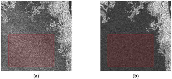
Figure 1.
Here, 512 × 512 pixel fragments of Sentinel-1 SAR images with VV (a) and VH (b) polarizations with manually selected quasi-homogeneous regions marked by red squares.
Spatial correlation can be detected and characterized in different ways: (a) by visualization and analysis of the 2D spatial auto-correlation function or its main cross-sections; (b) by analysis of the Fourier power spectrum; and (c) by analysis of the spatial spectra for other orthogonal transforms; all determined in the homogeneous image regions or estimated using some robust techniques able to eliminate or minimize the negative influence of image information content on the obtained estimates. Such an analysis was carried out, with results presented in [28,50,51]. It has been proven that speckle is spatially correlated, and the possibility of simulating speckle with the same characteristics as in Sentinel-1 images has been demonstrated [28].
For the quantitative analysis of the filtering efficiency, we used three types of metrics determined for simulated images. First, we determine metrics’ values for noisy images that were obtained by artificially introducing speckle with the aforementioned properties to noise-free images. Second, we calculate full-reference metrics’ values after filtering. Third, we estimate metrics’ “improvements” due to despeckling determined as , where and are metric values for denoised and true images, respectively.
For further analysis, we decided to use three metrics: conventional peak signal-to-noise ratio (PSNR), PSNR-HVS-M [52] (peak signal-to-noise ratio taking into account human vision system (HVS) and masking (M)), and the grayscale version of feature similarity index (FSIM) [53]. PSNR is the standard metric often used in analysis. The other two metrics are visual quality metrics that are among the best for characterizing grayscale (single-channel) image quality. As there are currently no universal visual quality metrics, we prefer using and analyzing two visual quality metrics based on different principles simultaneously. Moreover, the properties of these metrics are well studied. For example, PSNR and PSNR-HVS-M are both expressed in dB and their larger values are supposed to correspond to better quality. Distortion visibility thresholds for these metrics are established in [54]. It is also known that the difference in the quality of processed images of about 0.5 dB or larger can be noticed. Improvements of PSNR greater than 6 dB and of PSNR-HVS-M greater than 4 dB are needed to state with a high probability that SAR image visual quality has been improved due to filtering. The metric FSIM varies in the limits from 0 to 1 and it should be larger than 0.99 to show that noise or distortions are invisible [54]. This very rarely happens for SAR images, both original (noisy) and despeckled. Due to nonlinearity of FSIM, it is difficult to say what should be its improvement due to filtering to guarantee that a processed image has a better visual quality than the corresponding original one.
As it is known, the Lee filter output is expressed as
where is the output image, denotes the local mean in the scanning window centered on the -th pixel, denotes the central element in the window, is the variance of the pixel values in the current window.
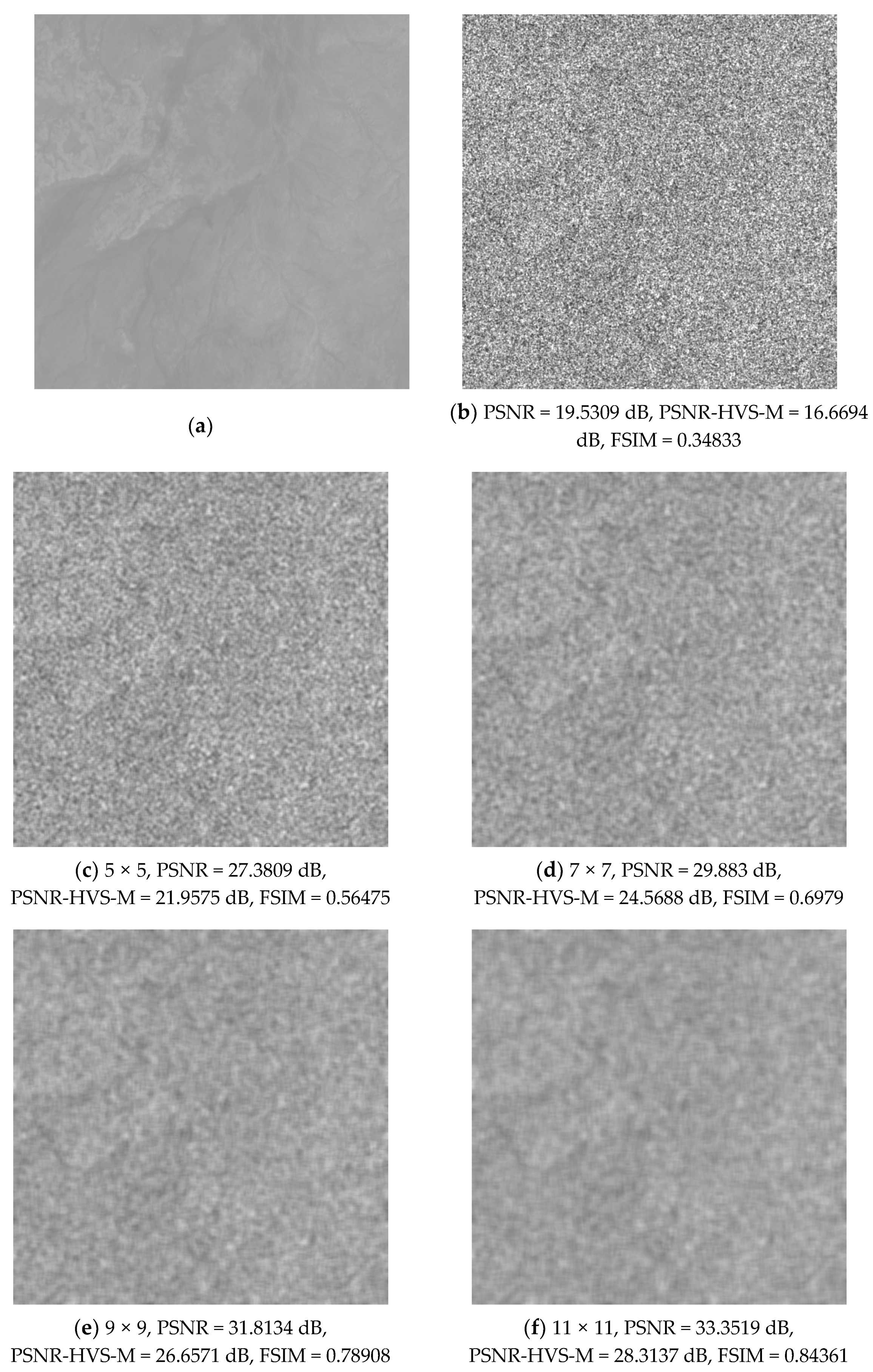
Below we present some examples of Lee filter outputs. Since there are no commonly accepted noise-free and noisy SAR test images, a common practice is either to create some artificial noise-free images or to use some practically noise-free images acquired by other sensors. In [28], we used component images from channels #5 and #11 of Sentinel-2 multispectral imager. Figure 2, Figure 3 and Figure 4 present some examples. Note that we consider four scanning window sizes: 5 × 5, 7 × 7, 9 × 9, and 11 × 11 pixels.
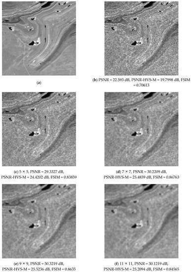
Figure 2.
Noise-free (a), noisy (b), and filtered (c–f) images (example 1).

Figure 3.
Noise-free (a), noisy (b), and filtered (c–f) images (example 2).
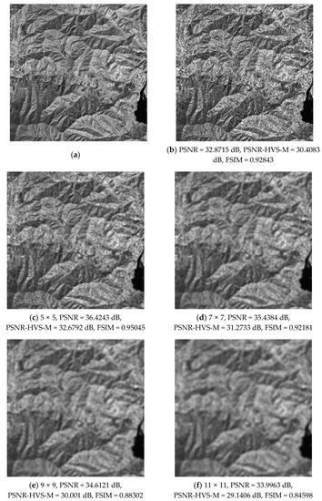
Figure 4.
Noise-free (a), noisy (b), and filtered (c–f) images (example 3).
Figure 2 gives an example of the situation when the processed image is of a middle complexity. The Lee filters with all four scanning window sizes produce improvements of all three considered metrics (compared to the noisy image, metrics’ values are placed below the corresponding images). The best (the largest) PSNR is provided by the 9 × 9 pixel scanning window, although the PSNRs for the 7 × 7 and 11 × 11 pixel windows are very close. The same holds for the metric PSNR-HVS-M, although the results for the 7 × 7 and 5 × 5 windows are very close. For FSIM, the best window size is 7 × 7 pixels. The results for the 5 × 5 window are the worst according to all criteria and indeed, speckle suppression is not enough. Concerning other the three output images, the opinions on their quality can differ from one expert to another.
Figure 3 presents a “marginal” case when the image is almost homogeneous. In this case, the metrics’ values steadily grow (improve) if the scanning window size increases. The largest improvements are observed for the 11 × 11 pixel window, while for PSNR and PSNR-HVS-M they reach almost 14 and 12 dB, respectively, clearly showing that the 11 × 11 window is the best choice. This is in good agreement with intuitive expectations since just efficient speckle suppression is the main requirement to image denoising in homogeneous image regions and such a property is achieved for filters with large scanning windows.
Another “marginal” case is demonstrated in Figure 4. The test image has a complex structure (is textural). Due to this, the best results are provided by the 5 × 5 scanning window according to all analyzed metrics. However, it is difficult to judge whether the visual quality has improved due to filtering or not, although metrics’ improvements are positive. If the scanning window size increases, the output image quality decreases. This is because edge/detail/texture preservation is the main property of the filter in the considered case, and as it is known, a larger scanning window usually results in less preservation of image features, and therefore, worse visual quality.
The presented examples confirm that the optimal window size strongly depends on image content and the quality metric used. General tendencies are the following. First, a smaller window should be applied for complex structure images. Second, for visual quality metrics, optimal scanning window size is either the same as the optimal size according to PSNR or slightly smaller. This is explained by two facts: (a) for visual quality metrics, edge/detail/texture preservation is “more important” than noise suppression in homogeneous regions; (b) a better edge/detail/texture preservation is usually provided by filters with smaller window sizes (for the same filter type). Third, differences in metric values for filters with different scanning windows can be sufficient. For example, FSIM in example 1 varies from 0.87 to 0.84, PSNR in example 2 varies from 27.4 dB to 33.4 dB, PSNR-HVS-M in example 3 varies from 32.7 dB to 29.1 dB. This shows that it can be reasonable to apply the optimal window size.
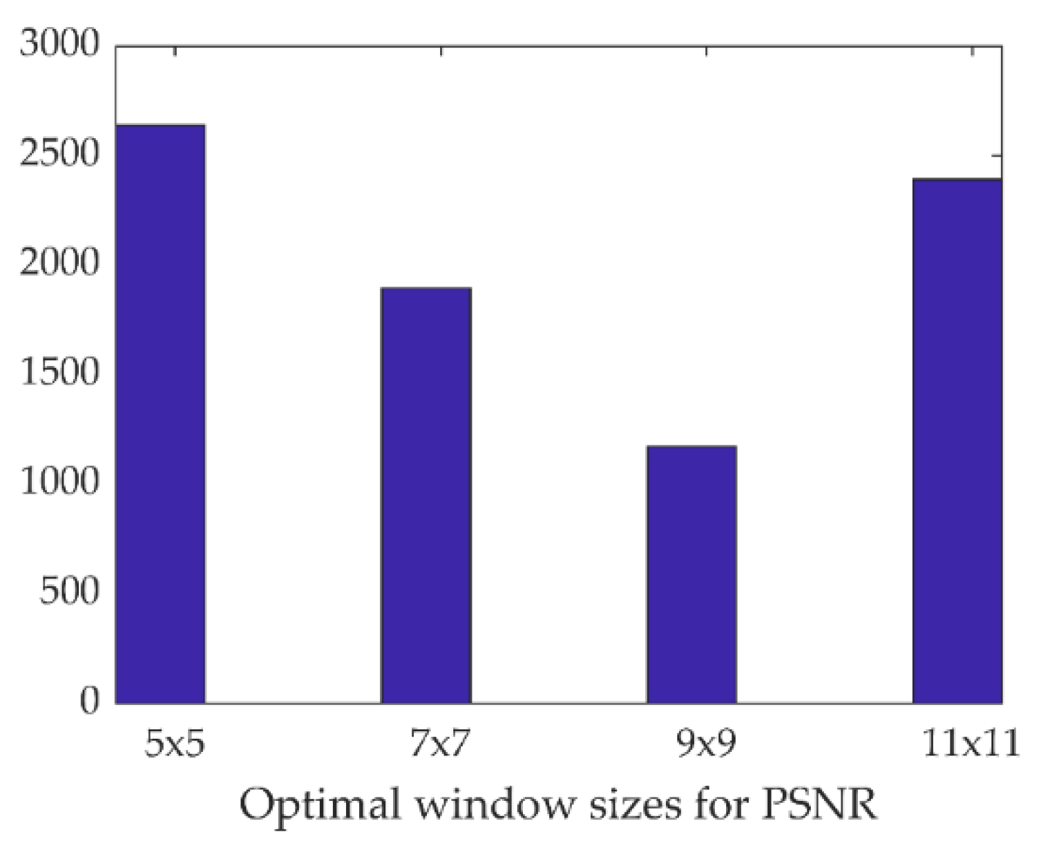
As we only considered "marginal" cases for which the necessity to choose (determine) the optimal window size is obvious, we also carried out additional study. First, we determined the “statistics” of each window size to be optimal. For this purpose, 8100 test images of size 512 × 512 pixels were employed. After adding speckle, filtering with four scanning window sizes was applied and the metrics’ values were calculated. For each metric, we determined how many times each window size provided the best results. Data obtained for all three considered metrics are given in Figure 5, Figure 6 and Figure 7. The plot in Figure 5 shows that, according to PSNR, the 5 × 5 and 11 × 11 windows more frequently appear than the 7 × 7 and 9 × 9 pixel windows.

Figure 5.
Numbers of test images with different optimal window sizes according to PSNR.

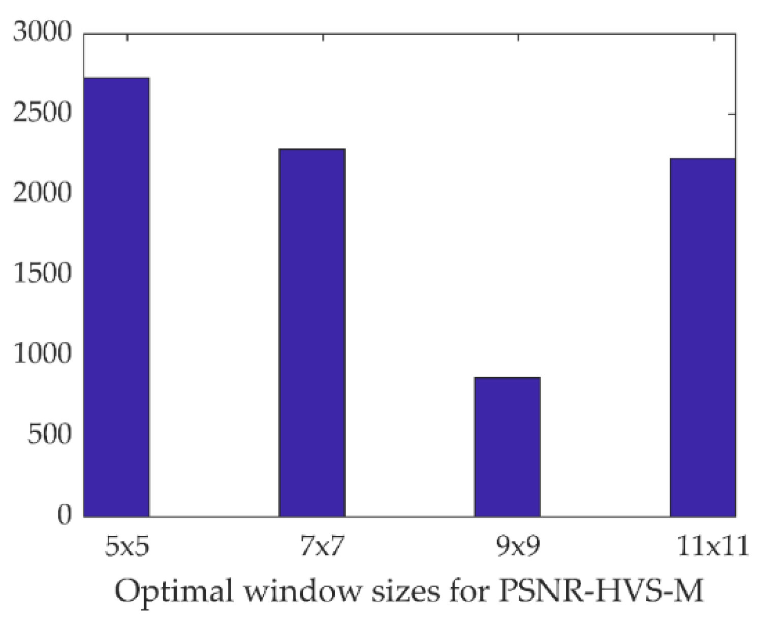
Figure 6.
Numbers of test images with different optimal window sizes according to PSNR-HVS-M.
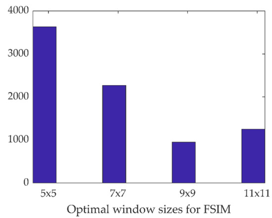
Figure 7.
Numbers of test images with different optimal window sizes according to FSIM.
Meanwhile, the analysis of the plots in Figure 6; Figure 7 demonstrates that, according to PSNR-HVS-M and FSIM, the 5 × 5 and 7 × 7 windows are better more often than the 9 × 9 and 11 × 11 windows. The reasons why this happens have been explained earlier. Note that, quite probably, the 3 × 3 or 13 × 13 windows can be optimal in some cases. However, our goal here is to prove that different window sizes can be optimal depending on image/noise properties and filtering efficiency criteria.
A global adaptation of window size is worth carrying out if the provided benefit is high. A benefit can be determined differently. We calculated the two following parameters:
where MaxPSNR and MaxPSNR-HVS-M are the maximal values (among four available) of output PSNR and PSNR-HVS-M, respectively, and the subscript relates to the scanning window size (PSNR5 means PSNR for 5 × 5 window).
∆PSNR = MaxPSNR − (PSNR5 + PSNR7 + PSNR9 + PSNR11)/4,
∆PSNR-HVS-M = MaxPSNR-HVS-M − (PSNR-HVS-M5 + PSNR-HVS-M7 +
+ PSNR-HVS-M9 + PSNR-HVS-M11)/4,
+ PSNR-HVS-M9 + PSNR-HVS-M11)/4,
The histogram of ∆PSNR is presented in Figure 8. It has the mode for ∆PSNR of about 0.4 dB. The minimal value is about 0.1 dB and the maximal value is about 3.7 dB. This means that a benefit due to the proper selection of optimal window size can be quite large.
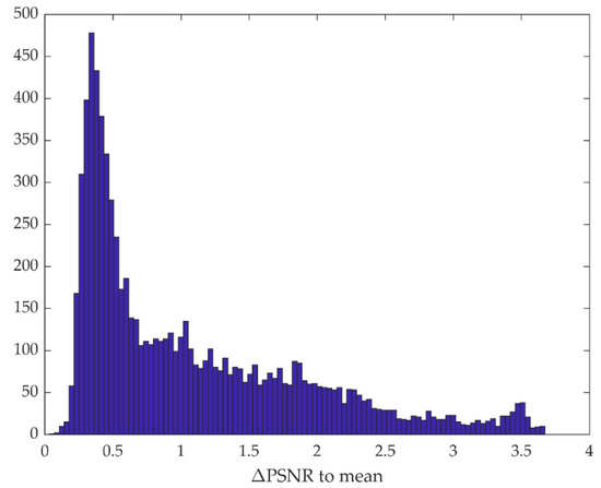
Figure 8.
Histogram of ∆PSNR for test images.
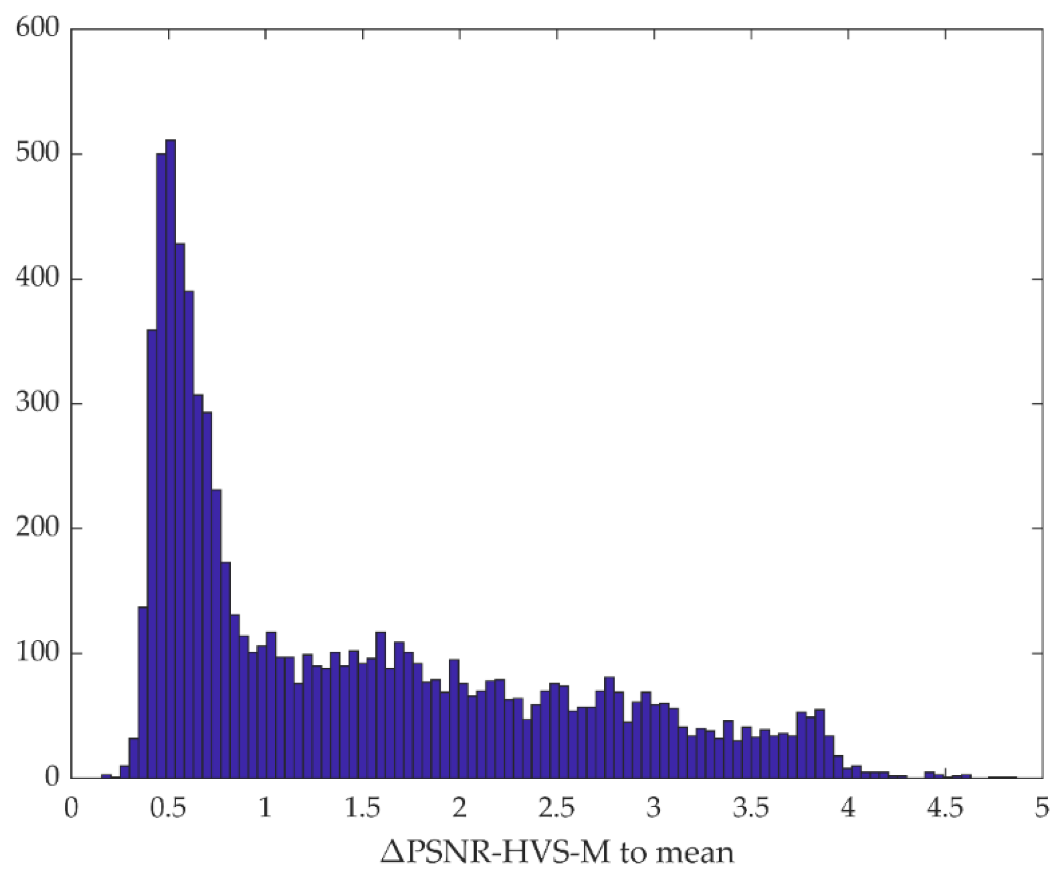
Similarly, Figure 9 represents the histogram of ∆PSNR-HVS-M. The distribution mode is about 0.5 dB, the minimal benefit is about 0.2 dB and the maximal one reaches almost 5 dB.

Figure 9.
Histogram of ∆PSNR-HVS-M for test images.
Thus, the first hypothesis put forward in Introduction is proven and it is worth selecting the optimal window size. To show that it is possible, we study how to predict filtering efficiency.
3. Filtering Efficiency Prediction Using Trained Neural Network
3.1. Proposed Approach
It was mentioned above that our approach is based on the prediction of filtering efficiency. We assume that there is a method and/or a tool that allows predicting filter efficiency in terms of some criteria (e.g., using a metric or several metrics). Then, filter efficiency can be evaluated (predicted) for a set of filter parameter values (e.g., window size for the local statistic Lee filter). Based on this prediction, it is possible to undertake a decision as to what value of the considered parameter to set in order to obtain an “optimal result” for a given image. The core of this approach is a neural network-based predictor trained off-line for test images that have approximately the same image and noise properties as real-life images to be further processed.
We briefly explain what this means and the requirements for such a prediction. Our first assumption is that there is at least one parameter able to adequately characterize filtering efficiency. This aspect has already been discussed and we will further suppose that improvements in PSNR, PSNR-HVS-M and FSIM (denoted as IPSNR, IPHVSM, IFSIM, respectively) can be considered as adequate metrics. Then, we assume that there are one or several parameters that are able to characterize image and noise properties. In general, these can be different parameters [27,28,48,49], with the main requirements as follows: (a) the parameters have to be informative, (b) they should be calculated easily and quickly. Finally, there should be a connection between the chosen output parameter(s) (predicted metric or metrics) and input parameter(s). This connection should allow estimating output parameter(s) using input one(s). A connection can be realized in different ways—as an analytic expression, as a regressor, or as a more complex tool, such as a support vector machine (SVM) or a neural network (NN).
Our previous experience in the design and analysis of filter efficiency prediction [27,28,48,49] has demonstrated the following:
- Even one input parameter (if it is informative and takes into account noise statistics or spectrum) is able to provide an accurate prediction of filtering efficiency for many different denoising techniques and criteria (metrics) [27,48];
- A joint use of several input parameters realized as a multi-parameter regression [48] or trained NN [28,49] usually leads to the sufficient improvement of prediction accuracy at the expense of the extra calculations needed.
3.2. Neural Network Input Parameters
It has been shown [49] that the improvements of many metrics can be accurately predicted for the 5x5 local statistic Lee filter using the trained NN. Recall here that the performance of any NN depends on many factors regardless of what functions are carried out by an NN (approximation, classification, recognition, etc.). These factors are the following: (a) NN structure and parameters (e.g., the number of hidden layers); (b) input parameters used and their number, (c) activation function type and parameters; (d) a methodology of NN training.
It is difficult to analyze the influence of all these factors within one paper. Due to this, we incorporated some knowledge and experience obtained in our previous works [33,48,49]. In particular, the different sets of input parameters have been considered in [48]. Originally, four groups of input parameters have been proposed.
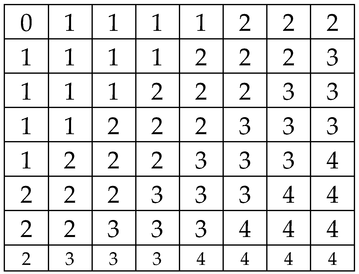
The first group includes sixteen parameters, all calculated in the discrete cosine transform (DCT) domain. A normalized spectral power was determined in four spectral areas of 8 × 8 pixel blocks marked by digits from 1 to 4 in Figure 10. Zero relates to the DC coefficient not used in the calculations.
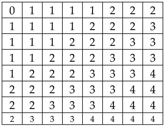
Figure 10.
Four spectral areas in the 2D DCT domain.
Four energy allocation parameters are expressed as
Here, and denote indices of DCT coefficients in a block ( ), () is an index of the -th spectral area (see Figure 10). In fact, the parameters characterize the distribution of energy between areas and they all are in the limits from 0 to 1. Having a set of determined for a certain number of blocks, four statistical parameters were calculated for each area: mean, variance, skewness, and kurtosis. Then, sixteen parameters (denoted as ) that take into account the spectral characteristics of both the true image and speckle are obtained.
The second group includes four input parameters. They all relate to image statistics in 8 × 8 pixel blocks. We denote them as (the mean, variance, skewness, and kurtosis of block means, respectively). They partly describe the image histogram.
The third group of input parameters has come from our previous experience in designing simple predictors [27]. The parameters are also based on data processing in 8 × 8 blocks. Let us estimate the probabilities in a -th block (where defined the total number of the considered blocks), where magnitudes of DCT coefficients are smaller than the corresponding frequency and signal-dependent thresholds:
where is the DCT normalized power spectrum, and denotes the -th block mean. After estimating , four statistical parameters (mean, variance, skewness and kurtosis) of these probabilities were calculated. We denote them as , respectively.
It was also supposed [48,49] that general image statistics can be useful. Due to this, four other parameters have been calculated: image mean, variance, skewness, and kurtosis (denoted as , respectively).
All 28 parameters that can be potentially employed as NN inputs can be calculated easily and quickly. DCT in 8 × 8 blocks is a fast operation; other operations are either simple arithmetic or logic operations. A part of them can be calculated in parallel or in a pipeline manner. The essential acceleration of calculations also stems from the fact [27] that usually one can process data only in 1000 blocks placed randomly to obtain the required statistics with appropriate accuracy.
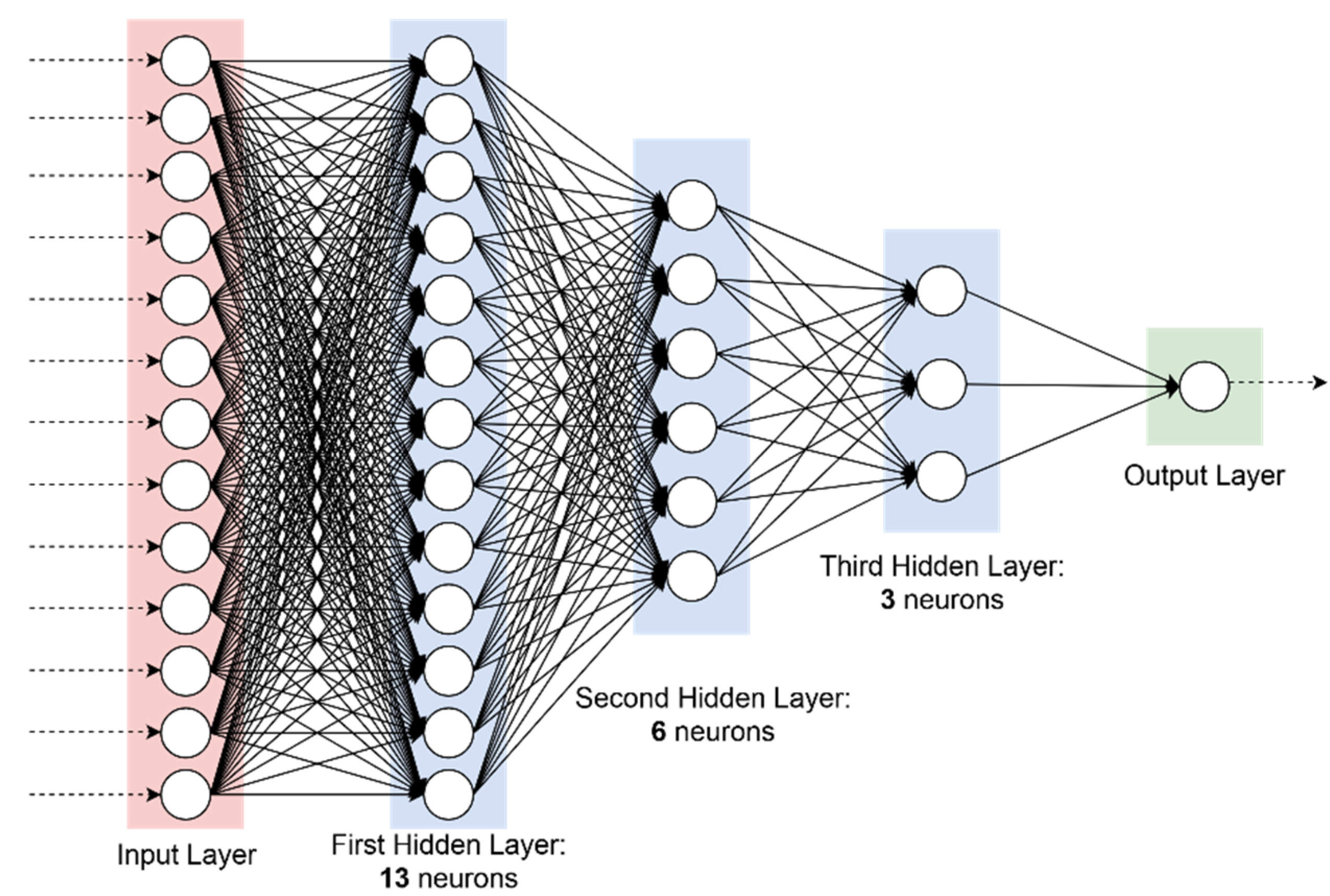
Numerous NN structures can be used. The multilayer perceptron (MLP) structure presented in Figure 11 is well recommended [28,49]. Studies carried out in [28] have shown that, without losing prediction accuracy, it is enough to use 13 input parameters, thus simplifying the NN-based predictor. These 13 input parameters are the following: and (see the description above).
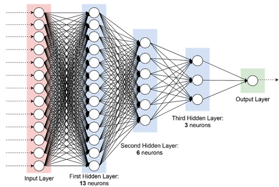
Figure 11.
Architecture of the multilayer perceptron.
4. NN Training Results
The MLP-based predictors were trained separately for each of three metrics (IPSNR, IPVHSM, IFSIM). As seen in Figure 11, the NN has three hidden layers. For all of them, hyperbolic tangent (tanh) activation function is used. The linear activation function is employed for the output layer. The MLP has 13 inputs introduced above. These input parameters must be calculated for each SAR image for which the prediction of filtering efficiency has to be done. The NN-based predictor has been trained by means of Bayesian regularization backpropagation.
The process of NN training and verification consists of four stages. The goals of the first two stages that concern self-dataset validation are to determine the final architecture and the number of training epochs. In turn, stages 3 and 4 relate to cross-dataset evaluation and checking the accuracy of the obtained predictors using data not exploited in the training process. One hundred high-quality cloudless images having total sizes of about 5500 × 5500 pixels have been obtained from components with a high SNR of multispectral RS data acquired by Sentinel-2. They were taken from channel #5 with the wavelength of about 700 nm and channel #11 with the wavelength of about 1600 nm. Using such large size fragments, images of the size 512 × 512 pixels were obtained (8100 images for each channel). These 512 × 512 pixel images were used as noise-free (true) images for which speckle distorted images were simulated.
At the preliminary stage, using noisy and corresponding true images, the metrics values were determined. Using noisy images, the input parameters considered in the previous section were determined and saved for all images. The filtered images were obtained and the quality metrics values for them were calculated. After obtaining all these data, the following actions to obtain and verify the NN performance were made. At the stage of the self-dataset validation, the optimal number of training epochs was established at 30. For the used architecture, it occurred to be equal to 30. The dataset was divided into two non-equal parts, 80% of test images have been employed for training and 20% of the remaining images for validation. The obtained training results are random. To overcome this pitfall, the validation was repeated 1000 times using the full permutation of the dataset. This allowed root mean square error (RMSE) and adjusted R2 [55] to be obtained after averaging to decide NN parameters. Smaller RMSE and larger adjusted correspond to better solutions.
Self-dataset validation results are presented in Table 1, where test images for channel #11 are used. As one can see, the prediction results are very good. IPSNR and IPHVSM are predicted with RMSE about 0.3 dB; adjusted
have practically identical values and they are in the limits from 0.976 to 0.989 showing that fitting carried out by the trained NN is excellent.

Table 1.
Self-dataset validation on the same Sentinel-2 data, channel #11.
If an NN is trained for one set of data and then applied to another set, the NN performance might radically worsen. To check this point, we performed cross-validations. Training was carried out for 6480 test images and parameters that characterize accuracy were estimated for another 1620 images. The obtained results are given in Table 2.

Table 2.
Cross-dataset evaluation for the same Sentinel-2 data, channel #11.
Cross dataset evaluation has been done for the same Sentinel-2 data from channel #11. Analysis shows that the RMSE values have slightly increased and the adjusted has slightly decreased compared to the corresponding data in Table 1. Meanwhile, the prediction accuracy remains very good. Usually, it is even more difficult for an NN to perform data processing if the sets used in training and verification differ sufficiently. In our case, this might happen if the NN is trained for test images composed of data in one channel of Sentinel-2 images and then applied to the test images composed of data in another channel. To check this case, we carried out the NN training on a Sentinel-2 dataset in channel #5 and then carried out cross-dataset evaluation on the dataset from Sentinel-2 channel #11. The obtained results are presented in Table 3.

Table 3.
Cross-dataset evaluation for Sentinel-2 data, channel #11 with training for Sentinel-2 data, channel #5.
The analysis of obtained results shows that the RMSE values are almost identical to the corresponding values in Table 2. The values of adjusted have slightly decreased compared to the corresponding data in Table 2. Nevertheless, the prediction is accurate enough. It is sufficiently better than that for predictors based on a single input parameter [27] and two input parameters [48]. We associate this benefit with two factors. First, the NN uses more input parameters that employ information on image statistics. Second, the NN exploits information about speckle spectral properties by means of input parameters and . The main parameters that characterize prediction accuracy for the Lee filter versions with different scanning window sizes are approximately the same as for the DCT-based filter analyzed in the paper [28]. Thus, we can conclude that there is a certain generality to the approach to filter efficiency prediction considered in this paper.
Hence, the second and the third hypotheses given in the Introduction are also proven. The high accuracy of prediction is provided compared to the simpler approach to prediction [27]. This is particularly due to taking into account the speckle statistical and spectral properties incorporated by input parameters that are among the most informative.
Now, the question is the following: is the attained accuracy of filter efficiency prediction enough for the adaptive selection of the Lee filter scanning window size?
5. Adaptive Selection of Window Size
There are several ways to adapt the filter window for a given image to its content based on prediction:
- To perform prediction for only one parameter, e.g., IPSNR, for all possible scanning window sizes, and to choose the window size for which the predicted metric (e.g., IPSNR) is the largest.
- To jointly analyze two or three metrics (e.g., IPSNR and IPHVSM or IPSNR, IPHVSM, and IFSIM) and undertake a decision (there probably are many algorithms to do this).
- To obtain three decisions based on the separate analysis of IPSNR, IPHVSM, and IFSIM as in the first item and then to apply the majority vote algorithm of some other decision rule.
Below, we concentrate on the way described in item 1 as the simplest solution, leaving other options for the future.
Decisions can be characterized in various ways. We are mainly interested in two aspects—what is the probability of a correct decision for our approach and what happens if the undertaken decision is wrong, i.e., if an incorrect scanning window size is decided to be used. The probabilities of correct decisions have been determined for self-dataset validation and cross-dataset evaluation. For the self-dataset validation stage, the probability of a correct decision is approximately equal to 0.9 for IPSNR, 0.918 for IPHVSM, and 0.907 for IFSIM. Thus, a high probability of correct decisions has been reached.
For the cross-dataset evaluation in channel (#11), the probability is equal to 0.898 for IPSNR, 0.916 for IPHVSM, and 0.901 for IFSIM. For cross-dataset evaluation with channel (#5), the probability of a correct decision is 0.857 for IPSNR, 0.899 for IPHVSM, and 0.877 for IFSIM. For cross-dataset evaluation with another channel (#5), the probability of a correct decision for IPSNR equals to 0.857; for IPHVSM—to 0.899, and for IFSIM—to 0.877. All probabilities are high enough.
Let us now see what happens if a wrong decision is undertaken. Clearly, this must lead to a reduction in filtering efficiency. Hence, we estimated the differences in metrics values for the optimal (maximally attainable) metric value and the one produced in the case of wrong decision. The distribution of such differences for IPSNR is presented in Figure 12. Most differences are very small (less than 0.2 dB), so erroneous decision is not a problem. Meanwhile, there a few (six) cases where differences exceed 0.5 dB.
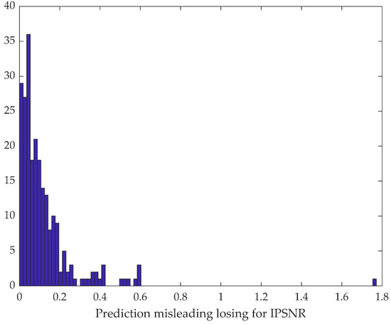
Figure 12.
Histogram of differences between the optimal and produced IPSNR in cases of wrong decisions.
Similarly, Figure 13 represents the distribution for differences between the optimal IPHVSM and the corresponding values produced in the cases of wrong decisions. Again, most differences are very small and do not exceed 0.2 dB. There are only two test images for which the differences are larger than 0.5 dB. Figure 14 shows the differences for IFSIM. Mostly, the differences are very small (less than 0.005). There are only three cases when the differences exceed 0.01.
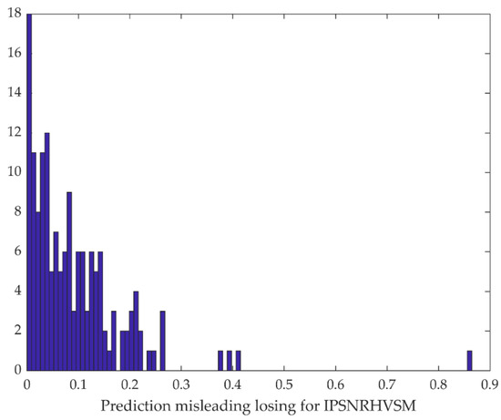
Figure 13.
Histogram of differences between the optimal and produced IPHVM in cases of wrong decisions.
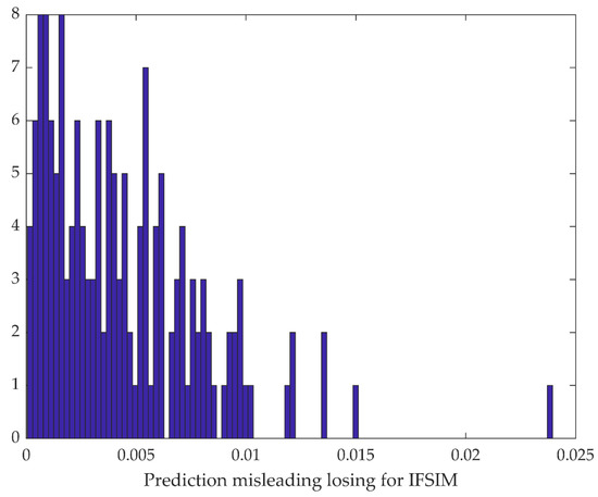
Figure 14.
Histogram of differences between the optimal and produced IFSIM in cases of wrong decisions.
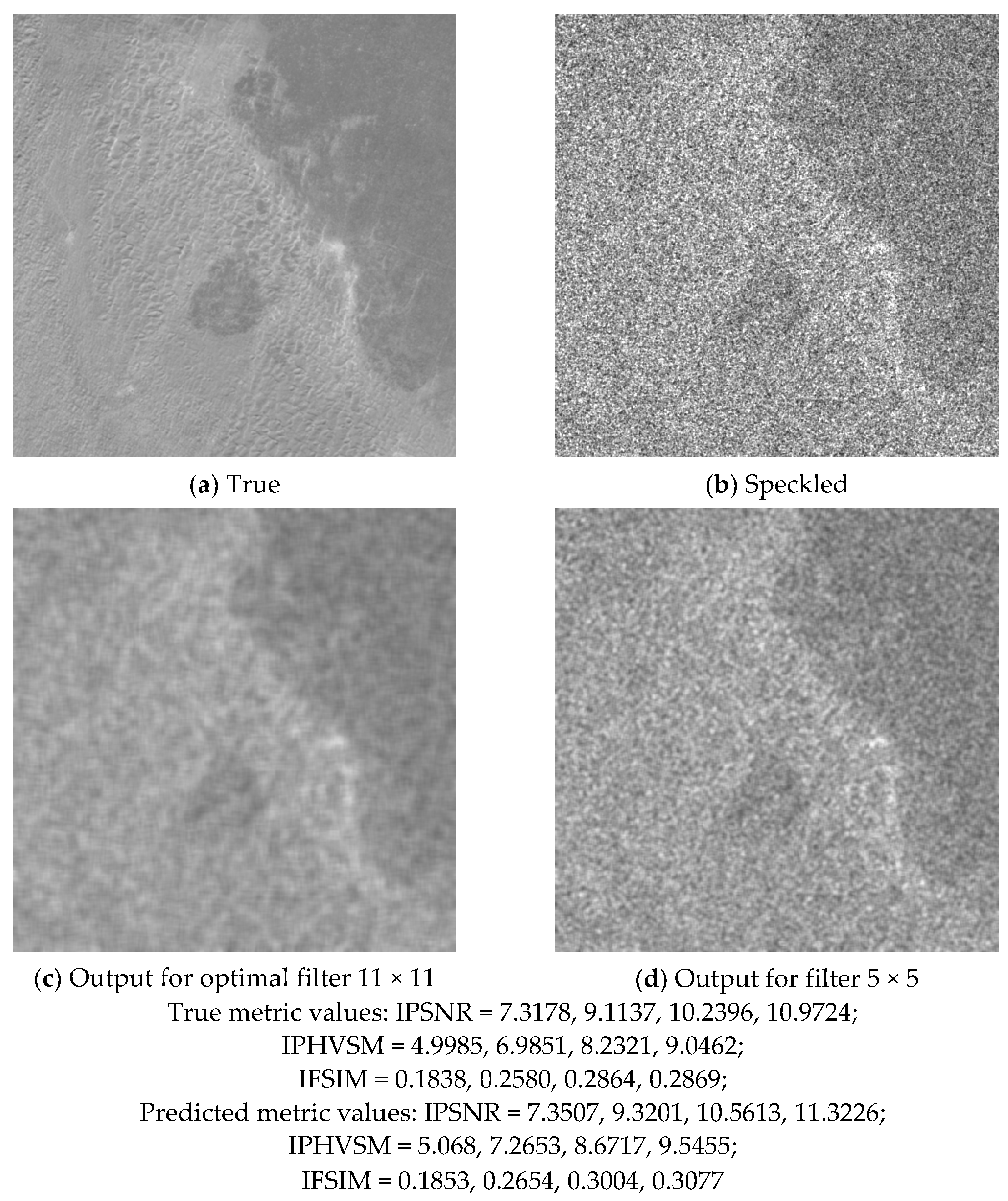
Let us present some examples of undertaking correct decisions (according to any considered metric). Figure 15 shows the true image (a); the speckled image (b); the optimal filter output for the 11 × 11 scanning window (c); and the filter output for the 5 × 5 scanning window that is surely not the best choice. In addition, we give all true and all predicted metric values. In this example, all true and the corresponding predicted values are close to each other. Meanwhile, all predicted values are slightly larger than the corresponding true values.

Figure 15.
The true image (a); the speckled image (b); the optimal filter output for the 11 × 11 scanning window (c); and the filter output for the 5 × 5 scanning window (d).
Note that for the examples given in Figure 2, Figure 3 and Figure 4, the optimal and the recommended window sizes coincide.
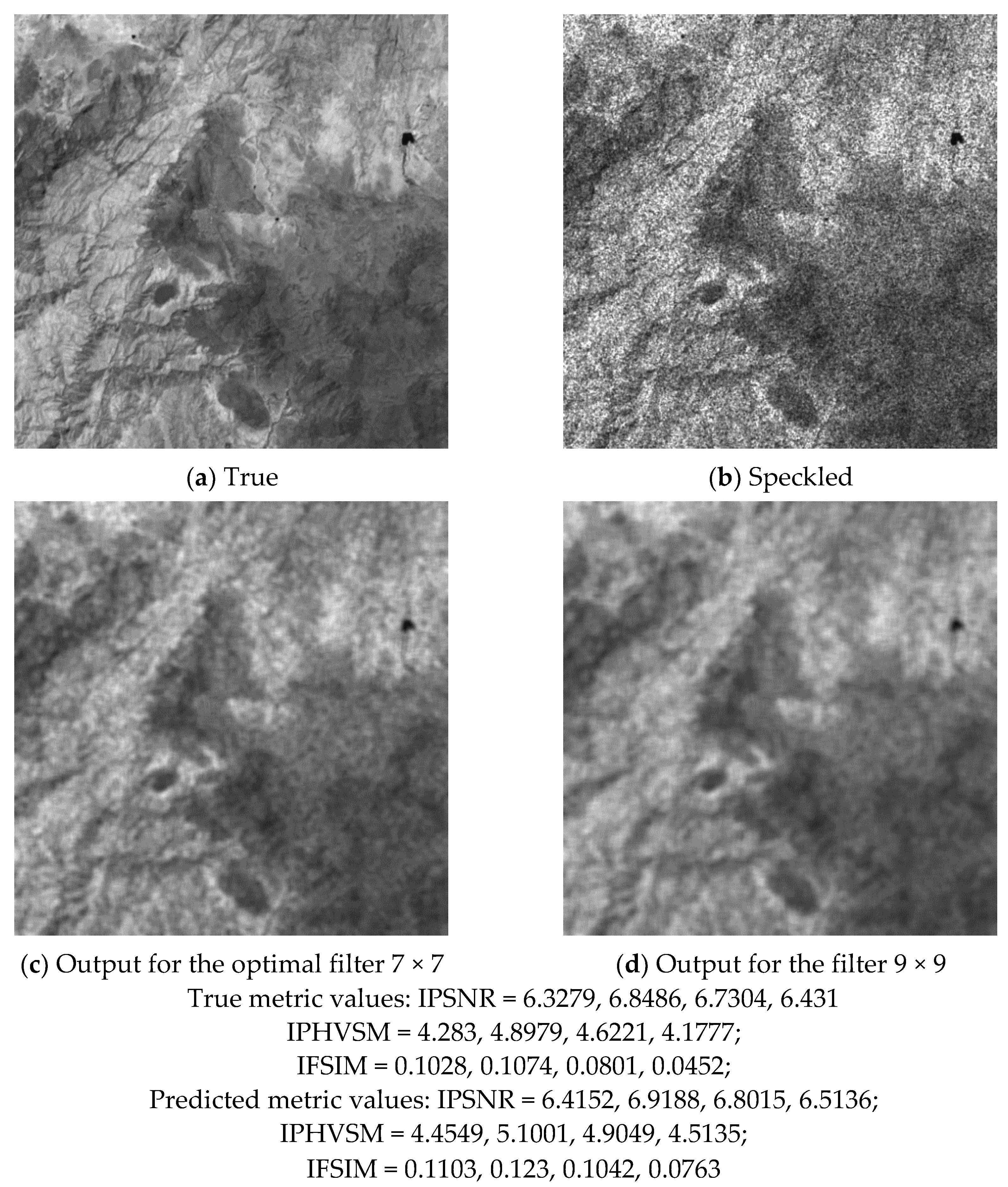
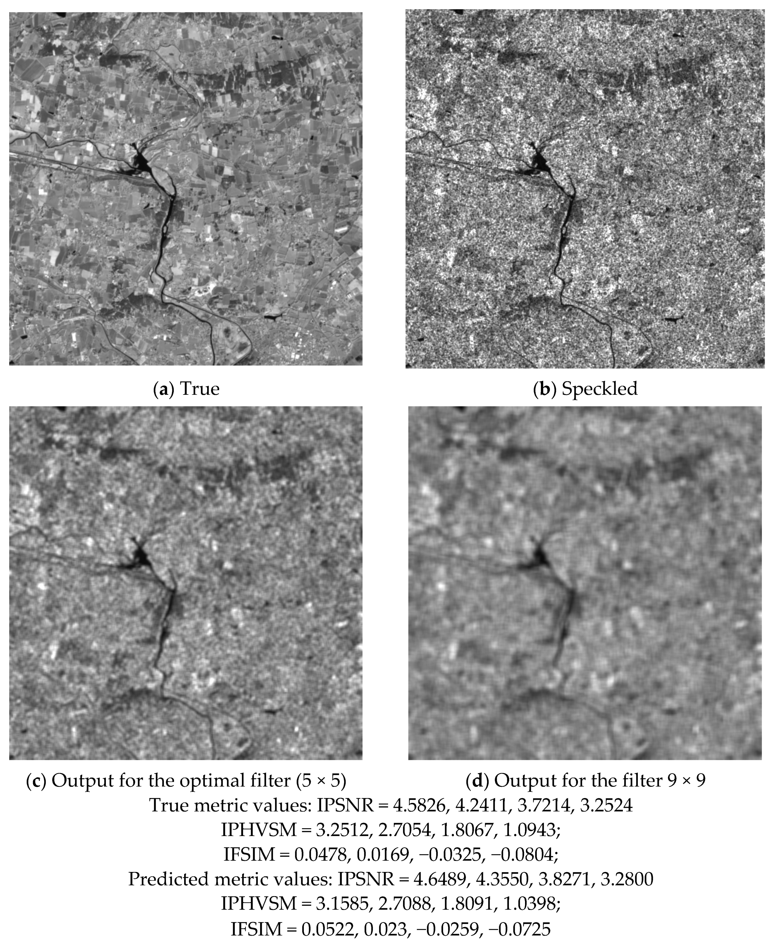
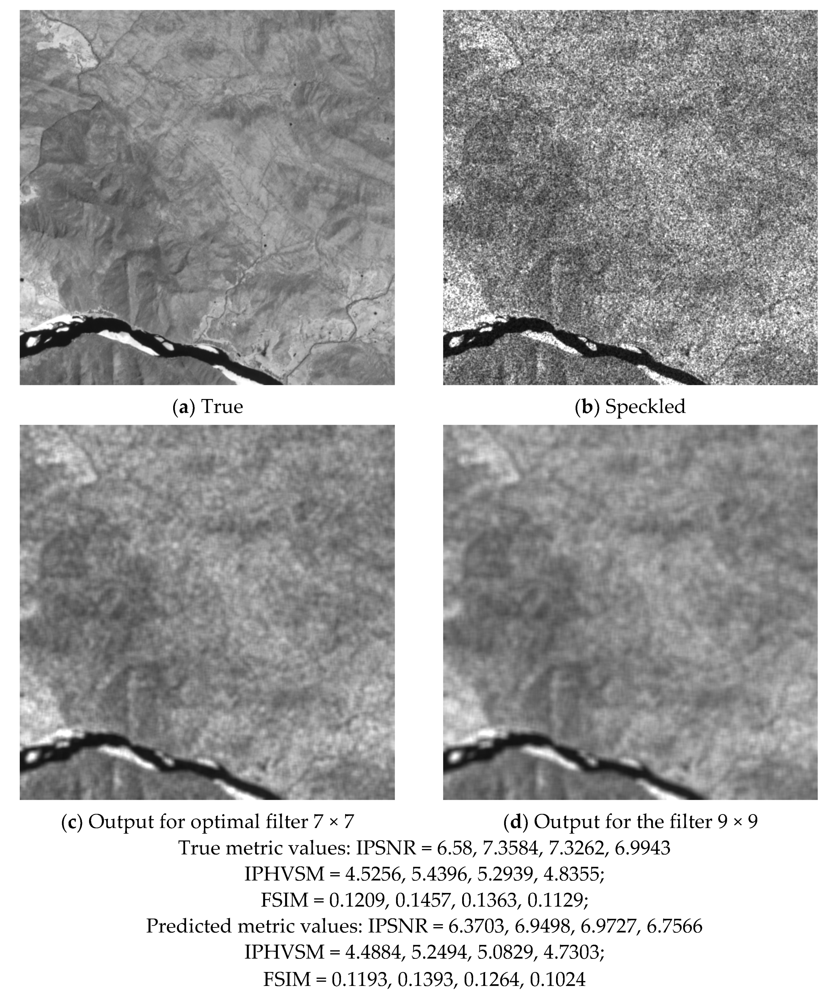
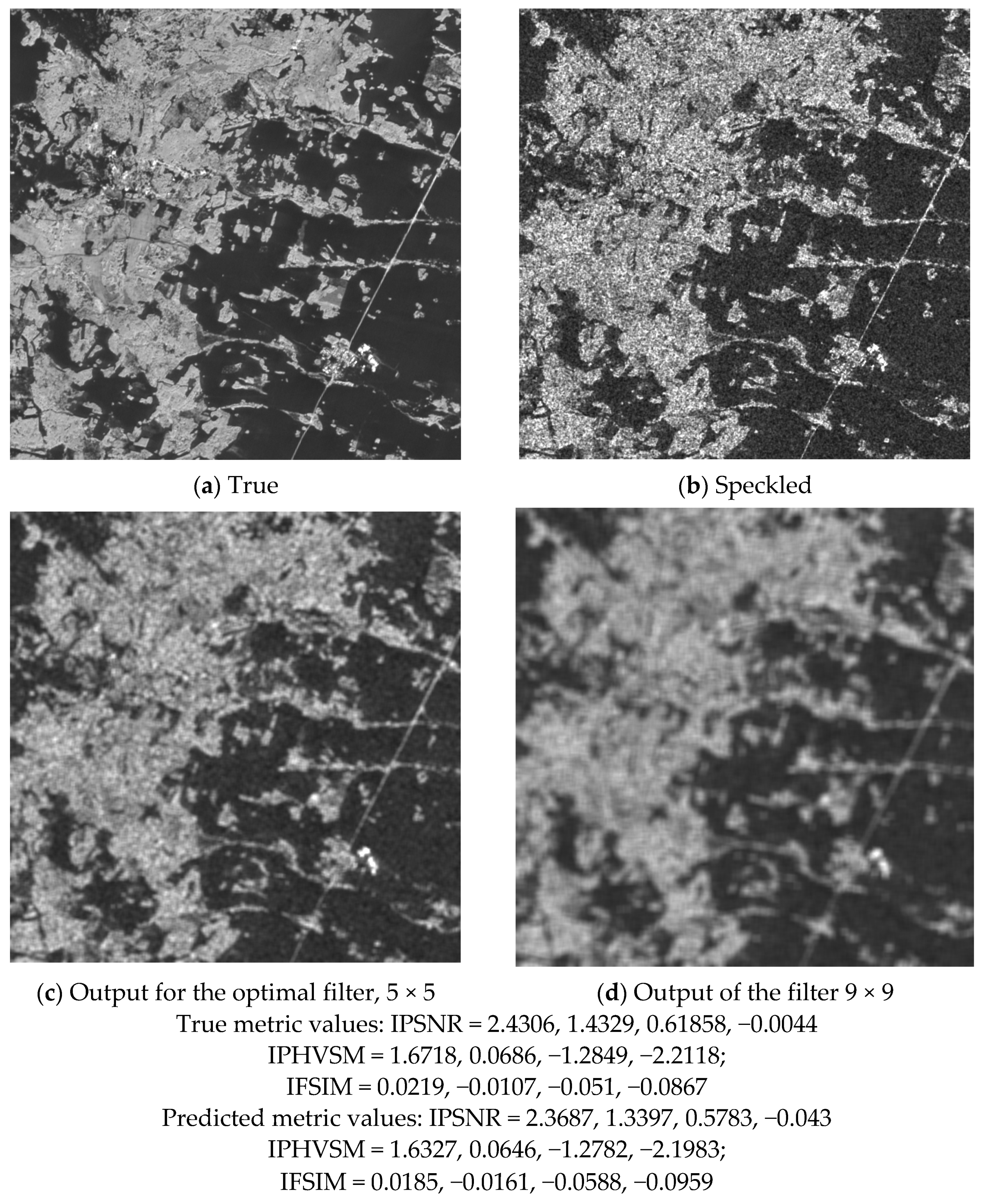
Figure 16 and Figure 17 show two more examples. For the image in Figure 16, the 7 × 7 window is the best choice according to both the true and predicted values of all three metrics, although the 9 × 9 window produces good outcomes as well. For the image in Figure 17, the 5 × 5 window is the best choice according to all three metrics, both true and predicted. The use of the 9 × 9 window leads to oversmoothed output. Note that IFSIM can be negative, indicating image quality degradation due to filtering.
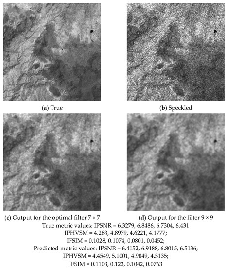
Figure 16.
The true image (a); the speckled image (b); the optimal filter output for the 7 × 7 scanning window (c); and the filter output for the 9 × 9 scanning window (d).
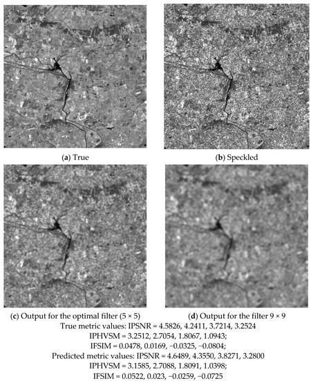
Figure 17.
The true image (a); the speckled image (b); the optimal filter output for the 5 × 5 scanning window (c); and the filter output for the 9 × 9 scanning window (d).
Figure 18 shows an example of a wrong decision. According to the predicted IPSNR, one must use the 9 × 9 window. Meanwhile, according to the true IPSNR, the 7 × 7 window is the best choice (the predicted IPHVSM and IFSIM are in favor of the 7 × 7 window too). However, in this case, the use of the 9 × 9 window does not lead to a considerably negative effect.

Figure 18.
The true image (a); the speckled image (b); the optimal filter output for the 7 × 7 scanning window (c); and the filter output for the 9 × 9 scanning window (d).
Figure 19 demonstrates one more interesting case. Obviously, the 5 × 5 window is the best choice. Meanwhile, for the 9 × 9 window, both true and predicted PSNR are close to zero while IPHVS and IFSIM are negative. In this case, when filtering by 9 × 9, the Lee filter is useless.
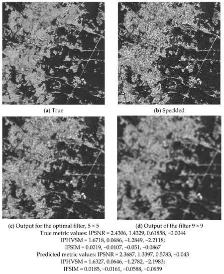
Figure 19.
The true image (a); the speckled image (b); the optimal filter output for the 5 × 5 scanning window (c); and the filter output for the 9 × 9 scanning window (d).
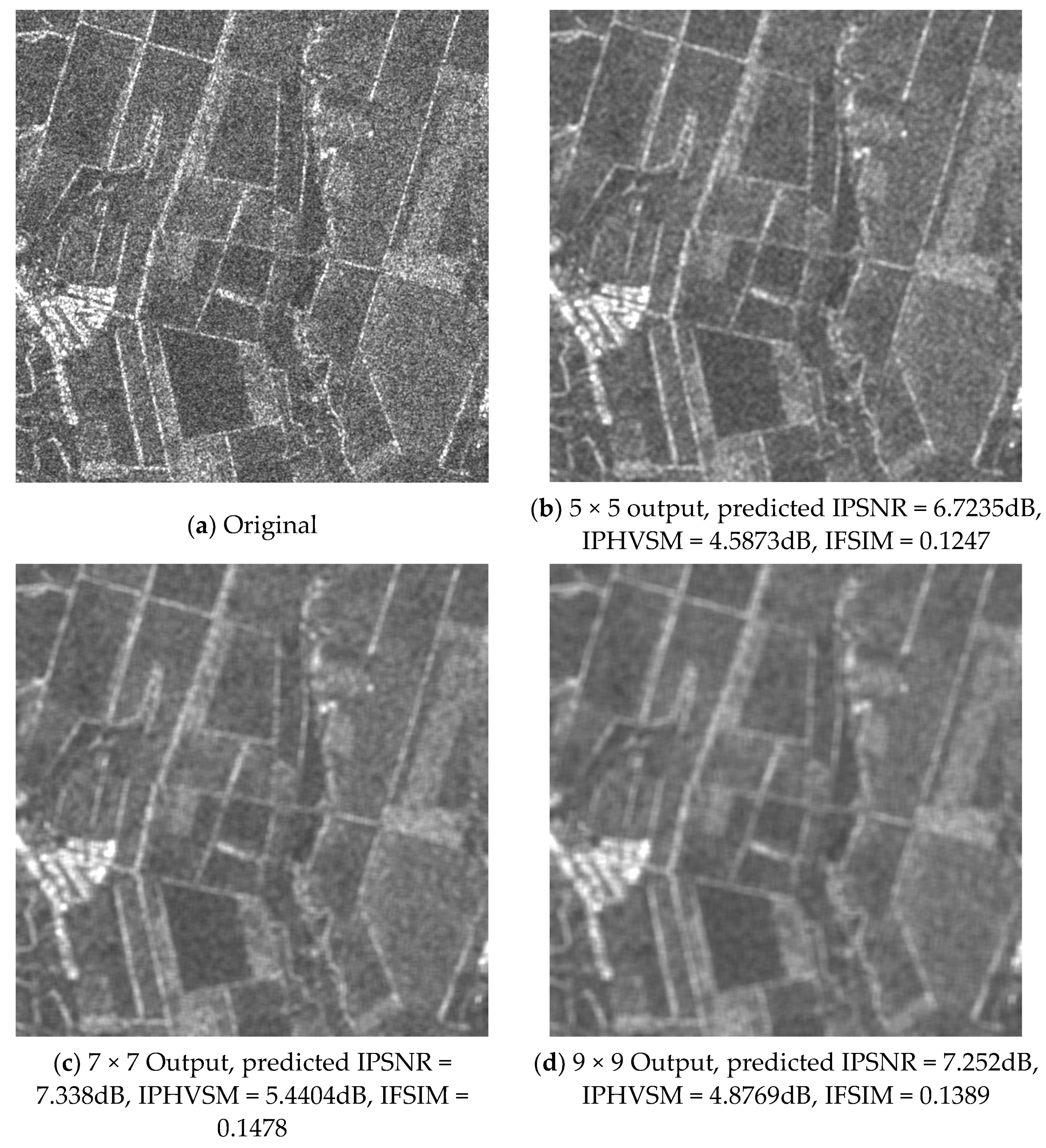
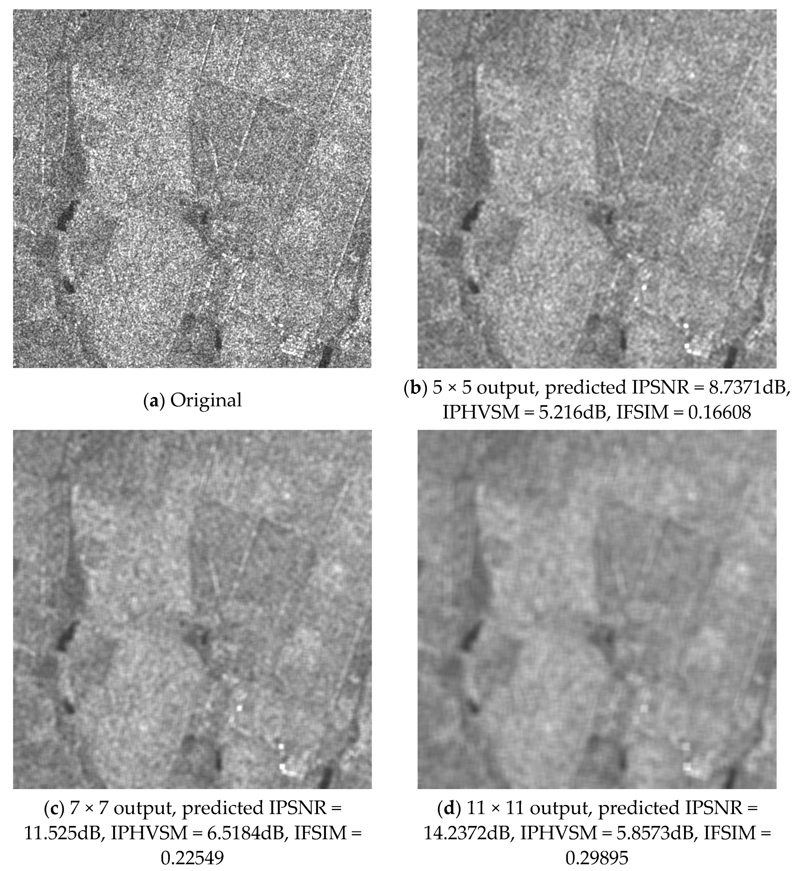
Let us give three real-life examples. Figure 20 shows an example for a real-life Sentinel-1 image of size 512 × 512 pixels. Since we do not have the true image in this case, we can demonstrate the results only visually and analyze them. The original (noisy) image was processed by the Lee filter with scanning window sizes of 5 × 5 (b); 7 × 7 (c); and 9 × 9 (d) pixels. The predicted metric values are given under the corresponding outputs. According to these, the 7 × 7 window size is the best and, in our opinion, this correlates with a visual analysis.

Figure 20.
The original Sentinel-1 image (a); and the outputs of the 5 × 5 (b); 7 × 7 (c); and 9 × 9 (d) Lee filters.
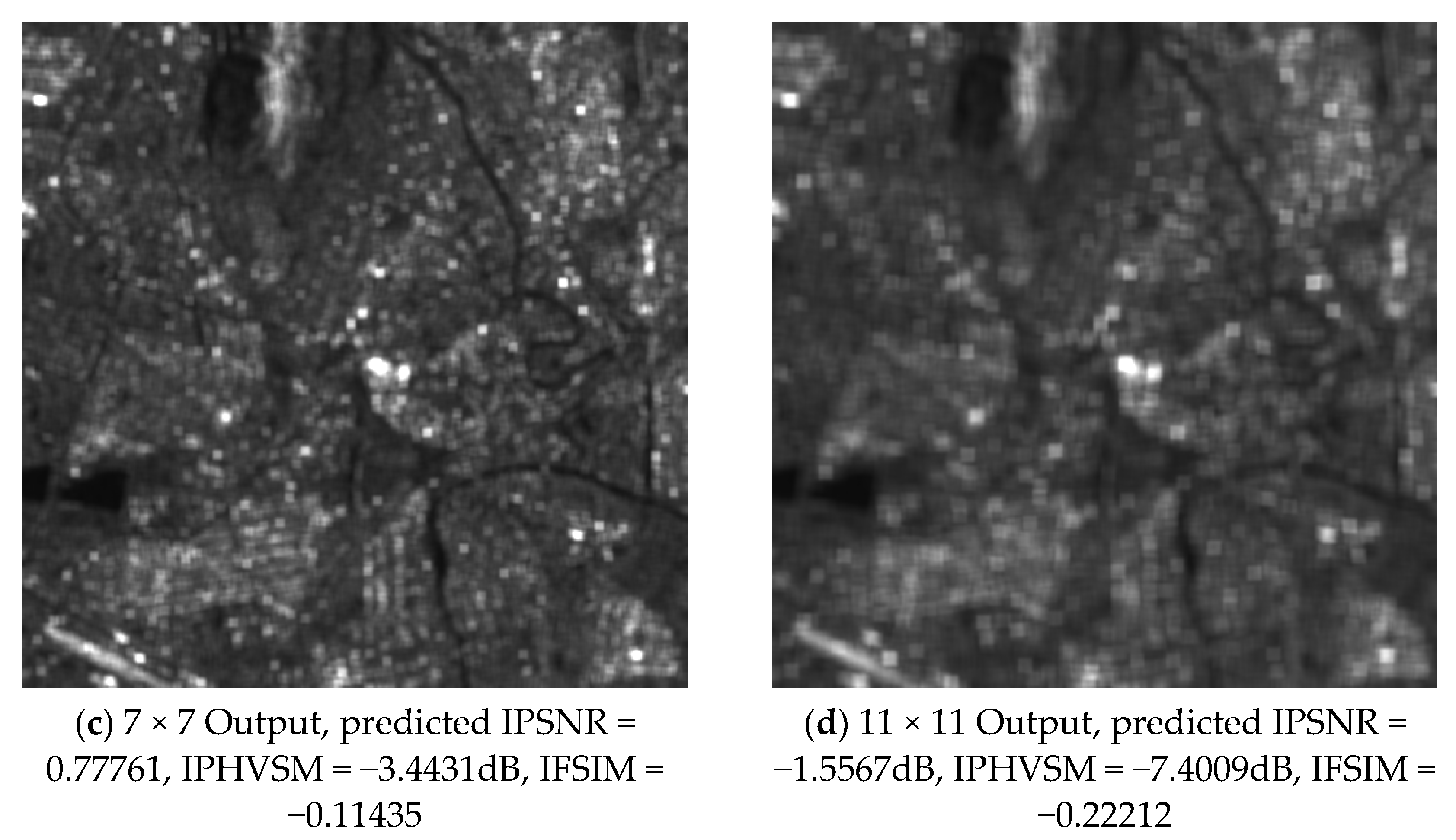
Another example is given in Figure 21. In this case, the image contains a lot of small-sized details. According to IPSNR, the despeckling produces a small improvement for the scanning windows of 5 × 5 and 7 × 7 pixels. However, according to visual quality metrics, the despeckling leads to image degradation for all three considered window sizes and this, in our opinion, is in agreement with visual inspection. Maybe, the use of the 3 × 3 pixel window can be a compromise.
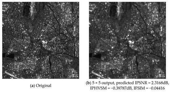

Figure 21.
The original Sentinel-1 image (a); and the outputs of the 5 × 5 (b); 7 × 7 (c); and 11 × 11 (d) Lee filters.
Finally, Figure 22 shows an image with large homogeneous regions. According to IPSNR and IFSIM, the 11 × 11 window is the best, but according to IPHVSM, the 7 × 7 pixel window is better. We prefer to agree with the latter variant.
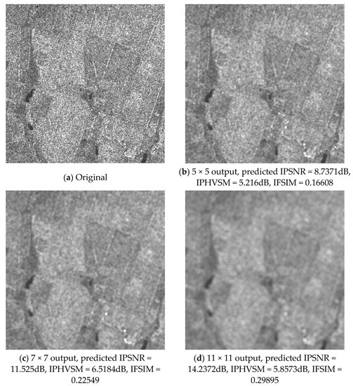
Figure 22.
The original Sentinel-1 image (a); and the outputs of 5 × 5 (b); 7 × 7 (c); and 11 × 11 (d) Lee filters.
6. Conclusions
The local statistic Lee filter is considered as a representative of the known de-speckling methods used in SAR image processing. It was shown that the scanning window size sufficiently influences the quality of output images. Thus, its adaptive setting seems expedient. We show how this size can be defined for a given image using filter efficiency prediction realized by a neural network. Many aspects of the neural network design and training are considered. A high prediction accuracy was demonstrated for three quality metrics. It was shown that the correct decisions can be undertaken with high probability (exceeding 0.85). The cases of undertaking wrong decisions are studied as well. It is shown that, in most situations, the negative outcomes of such decisions are negligible. Examples of simulated and real-life images are presented to explain the problem and give details concerning the proposed solutions (see data in Supplementary Materials Section).
We empirically proved all three hypotheses stated in the Introduction. Due to the optimal setting of the filter window size, a considerable improvement of despeckling efficiency can be reached compared to the case of fixed setting. The optimal window size can be chosen based on efficiency prediction performed by the trained NN. The proposed approach presumes that the training must be carried out, taking into account statistical and spectral properties of speckle for the considered class of SAR images.
If so, the question of universality of the proposed approach arises. The speckle statistical properties influence input signal-to-noise ratios of acquired images that, in turn, impact filtering efficiency [27] and other performance characteristics of RS image processing [56]. We adapted our NN predictor to the statistical and spectral characteristics of the speckle for five-look Sentinel SAR images and this is one reason why the high accuracy of prediction was provided. Therefore, we can currently talk about the universality of our approach in the sense that the same preliminary study and training can be carried out for other types of SAR images, e.g., for single-look TerraSAR-X images. Meanwhile, it is also possible to find such input parameters for a trained network that can be quite insensitive to the possible changes of speckle statistics and spatial spectrum.
Supplementary Materials
All materials and supplementary visualization will be available online at https://github.com/asrubel/Lee_filter_pred.
Author Contributions
Conceptualization, O.R. and V.L.; methodology, V.L.; software, O.R. and A.R.; validation, A.R.; formal analysis, K.E.; investigation, O.R.; resources, A.R.; data curation, O.R.; writing—original draft preparation, V.L.; writing—review and editing, K.E.; visualization, O.R.; supervision, K.E. All authors have read and agreed to the published version of the manuscript.
Funding
This research received no external funding.
Conflicts of Interest
The authors declare no conflict of interest.
References
- Schowengerdt, R.A. Remote Sensing: Models and Methods for Image Processing, 3rd ed.; Academic Press: San Diego, CA, USA, 2007. [Google Scholar]
- Lee, J.S.; Pottier, E. Polarimetric Radar Imaging: From Basics to Applications; CRC Press: Boca Raton, FL, USA, 2009; p. 422. [Google Scholar]
- Kussul, N.; Lemoine, G.; Gallego, F.J.; Skakun, S.; Lavreniuk, M.; Shelestov, A. Parcel-Based Crop Classification in Ukraine Using Landsat-8 Data and Sentinel-1A Data. IEEE J. Sel. Top. Appl. Earth Obs. Remote Sens. 2016, 9, 2500–2508. [Google Scholar] [CrossRef]
- Mullissa, A.G.; Persello, C.; Tolpekin, V. Fully Convolutional Networks for Multi-Temporal SAR Image Classification. In Proceedings of the IEEE International Geoscience and Remote Sensing Symposium, Valencia, Spain, 22–27 July 2018; pp. 3338–6635. [Google Scholar] [CrossRef]
- Joshi, N.; Baumann, M.; Ehammer, A.; Fensholt, R.; Grogan, K.; Hostert, P.; Jepsen, M.R.; Kuemmerle, T.; Meyfroidt, P.; Mitchard, E.T.A.; et al. A Review of the Application of Optical and Radar Remote Sensing Data Fusion to Land Use Mapping and Monitoring. Remote Sens. 2016, 8, 70. [Google Scholar] [CrossRef]
- Ferrentino, E.; Buono, A.; Nunziata, F.; Marino, A.; Migliaccio, M. On the Use of Multipolarization Satellite SAR Data for Coastline Extraction in Harsh Coastal Environments: The Case of Solway Firth. IEEE J. Sel. Top. Appl. Earth Obs. Remote Sens. 2021, 14, 249–257. [Google Scholar] [CrossRef]
- Nascimento, A.; Frery, A.; Cintra, R. Detecting Changes in Fully Polarimetric SAR Imagery with Statistical Information Theory. IEEE Trans. Geosci. Remote Sens. 2019, 57, 1380–1392. [Google Scholar] [CrossRef]
- Deledalle, C.; Denis, L.; Tabti, S.; Tupin, F. MuLoG, or How to Apply Gaussian Denoisers to Multi-Channel SAR Speckle Reduction? IEEE Trans. Image Process. 2017, 26, 4389–4403. [Google Scholar] [CrossRef]
- Arienzo, A.; Argenti, F.; Alparone, L.; Gherardelli, M. Accurate Despeckling and Estimation of Polarimetric Features by Means of a Spatial Decorrelation of the Noise in Complex PolSAR Data. Remote Sens. 2020, 12, 331. [Google Scholar] [CrossRef]
- Touzi, R. Review of Speckle Filtering in the Context of Estimation Theory. IEEE Trans. Geosci. Remote Sens. 2002, 40, 2392–2404. [Google Scholar] [CrossRef]
- Oliver, C.; Quegan, S. Understanding Synthetic Aperture Radar Images; SciTech Publishing: Raleigh, NC, USA, 2004. [Google Scholar]
- Lee, J. Digital Image Enhancement and Noise Filtering by Use of Local Statistics. IEEE Trans. Pattern Anal. Mach. Intell. 1980, PAMI-2, 165–168. [Google Scholar] [CrossRef] [PubMed]
- Frost, V.; Stiles, J.; Shanmugan, K.; Holtzman, J. A Model for Radar Images and Its Application to Adaptive Digital Filtering of Multiplicative Noise. IEEE Trans. Pattern Anal. Mach. Intell. 1982, PAMI-4, 157–166. [Google Scholar] [CrossRef]
- Argenti, F.; Lapini, A.; Bianchi, T.; Alparone, L. A Tutorial on Speckle Reduction in Synthetic Aperture Radar Images. IEEE Geosci. Remote Sens. Mag. 2013, 1, 6–35. [Google Scholar] [CrossRef]
- Kupidura, P. Comparison of Filters Dedicated to Speckle Suppression in SAR Images. Int. Arch. Photogramm. Remote Sens. Spat. Inf. Sci. 2016, XLI–B7, 269–276. [Google Scholar] [CrossRef]
- Lee, J.; Grunes, M.; Schuler, D.; Pottier, E.; Ferro-Famil, L. Scattering-model-based speckle filtering of polarimetric SAR data. IEEE Trans. Geosci. Remote Sens. 2006, 44, 176–187. [Google Scholar] [CrossRef]
- Cozzolino, D.; Parrilli, S.; Scarpa, G.; Poggi, G.; Verdoliva, L. Fast Adaptive Nonlocal SAR Despeckling. IEEE Geosci. Remote Sens. Lett. 2014, 11, 524–528. [Google Scholar] [CrossRef]
- Solbo, S.; Eltoft, T. A Stationary Wavelet-Domain Wiener Filter for Correlated Speckle. IEEE Trans. Geosci. Remote Sens. 2008, 46, 1219–1230. [Google Scholar] [CrossRef]
- Lee, J.S.; Wen, J.H.; Ainsworth, T.; Chen, K.S.; Chen, A. Improved Sigma Filter for Speckle Filtering of SAR Imagery. IEEE Trans. Geosci. Remote Sens. 2009, 47, 202–213. [Google Scholar] [CrossRef]
- Parrilli, S.; Poderico, M.; Angelino, C.; Verdoliva, L. A nonlocal SAR image denoising algorithm based on LLMMSE wavelet shrinkage. IEEE Trans. Geosci. Remote Sens. 2012, 50, 606–616. [Google Scholar] [CrossRef]
- Sun, Z.; Zhang, Z.; Chen, Y.; Liu, S.; Song, Y. Frost Filtering Algorithm of SAR Images with Adaptive Windowing and Adaptive Tuning Factor. IEEE Geosci. Remote Sens. Lett. 2020, 17, 1097–1101. [Google Scholar] [CrossRef]
- Wu, B.; Zhou, S.; Ji, K. A novel method of corner detector for SAR images based on Bilateral Filter. In Proceedings of the 2016 IEEE International Geoscience and Remote Sensing Symposium (IGARSS), Beijing, China, 10–15 July 2016; pp. 2734–2737. [Google Scholar] [CrossRef]
- Gupta, A.; Tripathi, A.; Bhateja, V. Despeckling of SAR Images via an Improved Anisotropic Diffusion Algorithm. Adv. Intell. Syst. Comput. 2013, 747–754. [Google Scholar] [CrossRef]
- Fracastoro, G.; Magli, E.; Poggi, G.; Scarpa, G.; Valsesia, D.; Verdoliva, L. Deep learning methods for SAR image despeckling: Trends and perspectives. arXiv 2020, arXiv:2012.05508. [Google Scholar]
- Tsymbal, O.; Lukin, V.; Ponomarenko, N.; Zelensky, A.; Egiazarian, K.; Astola, J. Three-state locally adaptive texture preserving filter for radar and optical image processing. EURASIP J. Appl. Signal Process. 2005, 2005, 1185–1204. [Google Scholar] [CrossRef]
- Chatterjee, P.; Milanfar, P. Is Denoising Dead? IEEE Trans. Image Process. 2010, 19, 895–911. [Google Scholar] [CrossRef]
- Rubel, O.; Lukin, V.; de Medeiros, F. Prediction of Despeckling Efficiency of DCT-based filters Applied to SAR Images. In Proceedings of the International Conference on Distributed Computing in Sensor Systems, Fortaleza, Brazil, 10–12 June 2015; pp. 159–168. [Google Scholar] [CrossRef]
- Rubel, O.; Lukin, V.; Rubel, A.; Egiazarian, K. NN-Based Prediction of Sentinel-1 SAR Image Filtering Efficiency. Geosciences 2019, 9, 290. [Google Scholar] [CrossRef]
- Rubel, O.; Lukin, V.; Egiazarian, K. Additive Spatially Correlated Noise Suppression by Robust Block Matching and Adaptive 3D Filtering. J. Imaging Sci. Technol. 2018, 62, 60401–1. [Google Scholar] [CrossRef]
- Goossens, B.; Pizurica, A.; Philips, W. Removal of Correlated Noise by Modeling the Signal of Interest in the Wavelet Domain. IEEE Trans. Image Process. 2009, 18, 1153–1165. [Google Scholar] [CrossRef] [PubMed]
- Colom, M.; Lebrun, M.; Buades, A.; Morel, J. Nonparametric Multiscale Blind Estimation of Intensity-Frequency-Dependent Noise. IEEE Trans. Image Process. 2015, 24, 3162–3175. [Google Scholar] [CrossRef] [PubMed]
- Dellepiane, S.; Angiati, E. Quality assessment of despeckled SAR images. In Proceedings of the 2011 IEEE International Geoscience and Remote Sensing Symposium 2011, Vancouver, BC, Canada, 24–29 July 2011; pp. 3803–3806. [Google Scholar] [CrossRef]
- Rubel, O.; Rubel, A.; Lukin, V.; Carli, M.; Egiazarian, K. Blind Prediction of Original Image Quality for Sentinel Sar Data. In Proceedings of the 2019 8th European Workshop on Visual Information Processing (EUVIP), Roma, Italy, 28–31 October 2019; pp. 105–110. [Google Scholar] [CrossRef]
- Wang, P.; Patel, V. Generating high quality visible images from SAR images using CNNs. In Proceedings of the IEEE Radar Conference (RadarConf18), Oklahoma City, OK, USA, 23–27 April 2018; pp. 570–575. [Google Scholar] [CrossRef]
- Lukin, V.; Abramov, S.; Krivenko, S.; Kurekin, A.; Pogrebnyak, O. Analysis of classification accuracy for pre-filtered multichannel remote sensing data. J. Expert Syst. Appl. 2013, 40, 6400–6411. [Google Scholar] [CrossRef]
- Congalton, R.G.; Green, K. Assessing the Accuracy of Remotely Sensed Data: Principles and Practices; CRC Press: Florida, FL, USA, 1999; ISBN 978-0-87371-986-5. [Google Scholar]
- Kumar, T.G.; Murugan, D.; Rajalakshmi, K.; Manish, T.I. Image enhancement and performance evaluation using various filters for IRS-P6 Satellite Liss IV remotely sensed data. Geofizika 2015, 179–189. [Google Scholar] [CrossRef]
- Yuan, T.; Zheng, X.; Hu, X.; Zhou, W.; Wang, W. A Method for the Evaluation of Image Quality According to the Recognition Effectiveness of Objects in the Optical Remote Sensing Image Using Machine Learning Algorithm. PLoS ONE 2014, 9, e86528. [Google Scholar] [CrossRef]
- Wang, Z.; Bovik, A.; Sheikh, H.; Simoncelli, E. Image Quality Assessment: From Error Visibility to Structural Similarity. IEEE Trans. Image Process. 2004, 13, 600–612. [Google Scholar] [CrossRef] [PubMed]
- Lin, W.; Jay Kuo, C.C. Perceptual visual quality metrics: A survey. J. Vis. Commun. Image Represent. 2011, 22, 297–312. [Google Scholar] [CrossRef]
- Chandler, D. Seven Challenges in Image Quality Assessment: Past, Present, and Future Research. ISRN Signal Process. 2013, 2013, 1–53. [Google Scholar] [CrossRef]
- Bosse, S.; Maniry, D.; Muller, K.; Wiegand, T.; Samek, W. Deep Neural Networks for No-Reference and Full-Reference Image Quality Assessment. IEEE Trans. Image Process. 2018, 27, 206–219. [Google Scholar] [CrossRef] [PubMed]
- European Space Agency. Earth Online. Available online: https://earth.esa.int/documents/653194/656796/Speckle_Filtering.pdf (accessed on 10 March 2021).
- Lee, J.; Ainsworth, T.; Wang, Y. A review of polarimetric SAR speckle filtering. In Proceedings of the 2017 IEEE International Geoscience and Remote Sensing Symposium (IGARSS), Fort Worth, TX, USA, 23–28 July 2017; pp. 5303–5306. [Google Scholar] [CrossRef]
- Milanfar, P. A Tour of Modern Image Filtering: New Insights and Methods, Both Practical and Theoretical. IEEE Signal Process. Mag. 2013, 30, 106–128. [Google Scholar] [CrossRef]
- Zemliachenko, A.; Lukin, V.; Djurovic, I.; Vozel, B. On potential to improve DCT-based denoising with local threshold. In Proceedings of the 2018 7th Mediterranean Conference on Embedded Computing (MECO), Budva, Montenegro, 10–14 June 2018; pp. 1–4. [Google Scholar] [CrossRef]
- Abramov, S.; Lukin, V.; Rubel, O.; Egiazarian, K. Prediction of performance of 2D DCT-based filter and adaptive selection of its parameters. In Proceedings of the Electronic Imaging 2020, Burlingame, CA, USA, 26–30 January 2020; pp. 319-1–319-7. [Google Scholar] [CrossRef]
- Rubel, O.; Abramov, S.; Lukin, V.; Egiazarian, K.; Vozel, B.; Pogrebnyak, A. Is Texture Denoising Efficiency Predictable? Int. J. Pattern Recognit. Artif. Intell. 2018, 32, 1860005. [Google Scholar] [CrossRef]
- Rubel, O.; Lukin, V.; Rubel, A.; Egiazarian, K. Prediction of Lee filter performance for Sentinel-1 SAR images. In Proceedings of the Electronic Imaging 2020, Burlingame, CA, USA, 26–30 January 2020; pp. 371-1–371-7. [Google Scholar] [CrossRef]
- Lukin, V.; Rubel, O.; Kozhemiakin, R.; Abramov, S.; Shelestov, A.; Lavreniuk, M.; Meretsky, M.; Vozel, B.; Chehdi, K. Despeckling of Multitemporal Sentinel SAR Images and Its Impact on Agricultural Area Classification. Recent Adv. Appl. Remote Sens. 2018. [Google Scholar] [CrossRef]
- Abramova, V.; Abramov, S.; Lukin, V.; Egiazarian, K. Blind Estimation of Speckle Characteristics for Sentinel Polarimetric Radar Images. In Proceedings of the IEEE Microwaves, Radar and Remote Sensing Symposium (MRRS), Kiev, Ukraine, 29–31 August 2017; pp. 263–266. [Google Scholar] [CrossRef]
- Ponomarenko, N.; Silvestri, F.; Egiazarian, K.; Carli, M.; Astola, J.; Lukin, V. On between-coefficient contrast masking of DCT basis functions. In Proceedings of the 3rd International Workshop on Video Processing and Quality Metrics for Consumer Electronics (VPQM), Scottsdale, AZ, USA, 25–26 January 2007; p. 4. [Google Scholar]
- Zhang, L.; Zhang, L.; Mou, X.; Zhang, D. FSIM: A feature similarity index for image quality assessment. IEEE Trans. Image Process. 2011, 20, 2378–2386. [Google Scholar] [CrossRef] [PubMed]
- Ponomarenko, N.; Lukin, V.; Astola, J.; Egiazarian, K. Analysis of HVS-Metrics’ Properties Using Color Image Database TID2013. Adv. Concepts Intell. Vis. Syst. 2015, 613–624. [Google Scholar] [CrossRef]
- Cameron, C.; Windmeijer, A. An R-squared measure of goodness of fit for some common nonlinear regression models. J. Econom. 1997, 77, 329–342. [Google Scholar] [CrossRef]
- Xian, G.; Shi, H.; Anderson, C.; Wu, Z. Assessment of the Impacts of Image Signal-to-Noise Ratios in Impervious Surface Mapping. Remote Sens. 2019, 11, 2603. [Google Scholar] [CrossRef]
Publisher’s Note: MDPI stays neutral with regard to jurisdictional claims in published maps and institutional affiliations. |
© 2021 by the authors. Licensee MDPI, Basel, Switzerland. This article is an open access article distributed under the terms and conditions of the Creative Commons Attribution (CC BY) license (https://creativecommons.org/licenses/by/4.0/).


