Article

Temperature and Relative Humidity Profile Retrieval from Fengyun-3D/HIRAS in the Arctic Region

1
Collaborative Innovation Center on Forecast and Evaluation of Meteorological Disasters, CMA Key Laboratory for Aerosol-Cloud-Precipitation, Nanjing University of Information Science & Technology, Nanjing 210044, China
2
School of Atmospheric Physics, Nanjing University of Information Science & Technology, Nanjing 210044, China
3
National Satellite Meteorological Center, Key Laboratory of Radiometric Calibration and Validation for Environmental Satellites, China Meteorological Administration, Beijing 100081, China
4
Department of Geography, Harokopio University of Athens, EI. Venizelou 70, Kallithea, 17671 Athens, Greece
*
Author to whom correspondence should be addressed.
Remote Sens. 2021, 13(10), 1884; https://doi.org/10.3390/rs13101884
Submission received: 15 April 2021 / Revised: 30 April 2021 / Accepted: 7 May 2021 / Published: 11 May 2021
(This article belongs to the Special Issue Remote Sensing Monitoring of Arctic Environments)

Abstract

:
The acquisition of real-time temperature and relative humidity (RH) profiles in the Arctic is of great significance for the study of the Arctic’s climate and Arctic scientific research. However, the operational algorithm of Fengyun-3D only takes into account areas within 60°N, the innovation of this work is that a new technique based on Neural Network (NN) algorithm was proposed, which can retrieve these parameters in real time from the Fengyun-3D Hyperspectral Infrared Radiation Atmospheric Sounding (HIRAS) observations in the Arctic region. Considering the difficulty of obtaining a large amount of actual observation (such as radiosonde) in the Arctic region, collocated ERA5 data from European Centre for Medium-Range Weather Forecasts (ECMWF) and HIRAS observations were used to train the neural networks (NNs). Brightness temperature and training targets were classified using two variables: season (warm season and cold season) and surface type (ocean and land). NNs-based retrievals were compared with ERA5 data and radiosonde observations (RAOBs) independent of the NN training sets. Results showed that (1) the NNs retrievals accuracy is generally higher on warm season and ocean; (2) the root-mean-square error (RMSE) of retrieved profiles is generally slightly higher in the RAOB comparisons than in the ERA5 comparisons, but the variation trend of errors with height is consistent; (3) the retrieved profiles by the NN method are closer to ERA5, comparing with the AIRS products. All the results demonstrated the potential value in time and space of NN algorithm in retrieving temperature and relative humidity profiles of the Arctic region from HIRAS observations under clear-sky conditions. As such, the proposed NN algorithm provides a valuable pathway for retrieving reliably temperature and RH profiles from HIRAS observations in the Arctic region, providing information of practical value in a wide spectrum of practical applications and research investigations alike.All in all, our work has important implications in broadening Fengyun-3D’s operational implementation range from within 60°N to the Arctic region.

Graphical Abstract

1. Introduction

Approximately 62% of the Arctic is covered by ocean, but as a result of global warming, the temperature in the Arctic is changing more dramatically in comparison to lower latitudes, and sea ice is shrinking fast [1]. As one of the global cold sources, the Arctic has an important impact not only on the flora and fauna of the area but also on the Earth’s climate regulation. In particular, it has an important impact on the climate in the middle and low latitudes of the northern hemisphere [2,3]. In recent years, the frequency of warming events in the troposphere has gradually exceeded that in the stratosphere in the Arctic region. Moreover, the trend of future climate change in the Arctic region is uncertain and complex, which requires further in-depth investigations on the climate variability in the Arctic region [4,5].
Information on atmospheric temperature and relative humidity is of key significance in disciplines including climate research, weather analysis and weather forecasting. At the same time, the temperature and humidity parameters of the atmosphere directly affect the interaction between the short-wave solar radiation and the long-wave radiation of the earth-air system, thus influencing the global radiation energy balance [6,7,8]. Therefore, it is of key importance to obtain information on the temperature and humidity profiles of the Arctic atmosphere timely. Radiosondes arethe standard approach for obtaining such measurements. However, the disadvantages of lower spatial and temporal resolution and lack of high-level data make it difficult to study climate change in the Arctic region. The development of satellite-borne infrared hyperspectral remote sensing detection [9,10,11,12] allows for overcoming the hurdles of traditionally implemented approaches. In addition, the higher spectral resolution it can get the narrow and steep weight function, which can improve the inversion accuracy. Therefore, it is a very important task to use satellite data with high spatial and temporal resolution to retrieve information on atmospheric profiles.
At present, there are two main inversion methods: physically-based retrieval method and statistical retrieval method. The former mainly obtains atmospheric parameters by solving the atmospheric radiation transmission equation in reverse. Wang et al. [13] retrieved atmospheric information by using physical retrieval algorithm from satellite-borne microwave sensor. Authors reported in their study that the background field required for inversion had obvious influence on the inversion results, especially on temperature. Guan et al. [14] used a one-dimensional variational algorithm to retrieval the temperature and humidity profile from Infrared Atmospheric Sounding Interferometer (IASI). Their findings showed that although the method could perform high-precision detection of atmospheric profiles, the process relied on the sounding data, which also had certain limitations. These studies reveal that although the physical inversion has high accuracy, the calculation process depends on the initial value, and it is time-consuming and complicated. At the same time, the inversion accuracy is also affected by the results of the radiative transfer model. Due to the special geographic location and complex weather conditions in the Arctic, it is more difficult to obtain accurate near-surface parameters. This will reduce the accuracy of the brightness temperature simulated by the forward model.
On the other hand, the statistical retrieval methods adopt the statistical relationship determined by the atmospheric profiles and the radiation in advance to retrieval atmospheric parameters, which can avoid the shortage of the forward model. The eigenvector regression algorithm is the most commonly used in statistical retrieval. Some scholars [15,16,17] used this approach to retrieve atmospheric profiles from Atmospheric Infrared Sounder (AIRS). Their results showed more accurate atmospheric temperature and humidity profiles retrieved from hyperspectral data. Although this method is fast, simple, stable, and easy to handle large data volume statistics, it does not consider the essence of radiation transmission and does not have the ability to deal with non-linearity, so the retrieval performance needs to be improved. Neural network (NN) technology not only has a strong ability to deal with non-linear problems and good fault tolerance, but also avoid the use of radiative transfer model, and more complicated calculation process. This algorithm can provide the numerical stability and efficiency of statistical methods without sacrificing the accuracy of model-based physical methods. Many scholars [18,19,20,21,22,23] have carried out research on retrieving atmospheric parameters using NN from satellite data. Zhang et al. [24] used NN to retrieval atmospheric profiles from simulated AIRS brightness temperature, and compared with the retrievals using eigenvector regression algorithm. Their results showed that the performance of artificial NN was better than the eigenvector inversion method. Huang et al. [25] used the NN algorithm and linear regression algorithm to study the microwave radiometer inversion method, and the results also revealed the NN technique can obtain higher accuracy than linear statistics. These studies have clearly evidenced the promising potential of using artificial NN in atmospheric parameters retrieval from satellite-borne instruments observations.
In purview of the above, the present study proposes a new NN algorithm to retrieve temperature and relative humidity profiles in the Arctic from Fengyun-3D/HIRAS Chinese second-generation polar orbit meteorological satellite. At present, the HIRAS operational retrieval algorithm only considers areas within 60°N and 60°S, thus it is urgently necessaryto develop an Arctic region algorithm separately, and this is where the present study contributes. ERA5 data and observations from HIRAS were used to train the NNs in our proposed technique. In evaluating the NNs performance, retrieved profiles by the proposed herein method was compared versus ERA5 data from ECMWF, RAOBs of the Arctic region (north of 60°N) from Wyoming website to calculate RMSE, mean error, and correlation coefficient [26,27]. Furthermore, additional comparisons were performed to assess the accuracy of the NNs retrievals with AIRS products referring to ERA5, which proves the advantages of the NNs retrieval algorithm for the Arctic region. The algorithm proposed in this study can obtain the temperature and RH profiles in the Arctic region synchronized with the satellite time, which can not only make up for the latency of ERA5 data, but also fill in the lack of radiosonde observations in the Arctic, especially on ocean.

2. Data and Methods

2.1. Data

2.1.1. Satellite Data

FengYun-3 is a Chinese second-generation sun-synchronous meteorological satellite [28]. HIRAS is the first infrared Fourier detection instrument carried on Fengyun-3D [29]. The main goal is to observe the infrared radiation emitted by the Earth-Atmosphere system with high spectral resolution in the 0.38–15.38 μm spectral range. The observations can be applied to the development of atmospheric temperature and humidity profiles retrieval products, numerical weather forecasting, and climate research. The observation spectrum information is shown in Table 1.
In the HIRAS instrument conventional mode, the scanning mirror works in cross-orbit scanning. There are 33 FORs (fields of regards) on each scan line, which contain 4 detection units arranged in a 2 × 2 array, and each detection unit is called FOV (field of view). The interval between each resident position of the earth observation is 3.6°, and the field angle of each probe observation is 1.1°, the instantaneous field size of the ground at the corresponding sub-point is about 16 km, the interval of each probe is 1.8°, corresponding to the ground distance of 26.17 km. In this study, the L1-level observation data passing through the Arctic region from May 2019 to April 2020 was used as input data for NNs modeling. All the satellite data used in our study can be obtained from the National Satellite Meteorological Center (http://satellite.nsmc.org.cn/PortalSite/Data/Satellite.aspx, accessed on 1 May 2019 to 30 April 2020) after user registration.

2.1.2. Re-Analysis Data

The reanalysis data has been obtained from ECMWF ERA5, collected as sample data set containing pressure levels data from land and ocean. The spatial resolution of the ERA5 is 0.25° × 0.25°. The output of the training set drawn from ERA5 temperature and relative humidity fields from May 2019 to April 2020 at 0:00 and 12:00 UTC was interpolated to the specified pressure layer (1–1000 hPa: 42 layers). Training targets in the Arctic were divided on the basis of two variables: season and surface type. The six months from April to October 2019 were defined as the Arctic warm season, and November 2019 to April 2020 were defined as the Arctic cold season. According to the LandSeaMask datasets of the observation instrument and sea-ice cover of surface data from ERA5 data, the training targets were divided into ocean and land. Selection of HIRAS observed data with collocated ERA5 was based on the following rationale: (1) The quality score (QA_Score) three bands of FOV should be 100. (2) The absolute distance between the position of ERA5 and HIRAS’FOV is less than 0.1°. (3) The time difference between reanalysis and HIRAS is less than 1 h.
Based on the data processing method mentioned above, a total of 44,043 samples were matched on land and 53,890 samples on the ocean, and the data division is shown in Table 2. Four fifths of the collected samples were used for modeling and the remaining for evaluating the accuracy of the NNs. The data distribution is shown in Figure 1a,b.

2.1.3. Sounding Data

As the ECMWF data is not the representation of the true state of the atmosphere, and the radiosonde data is the closest to the real state of the atmosphere at present, NNs performance was also compared versus radiosondes on land from May 2019 to April 2020 at 00:00 and 12:00 UTC (from the University of Wyoming). The RAOBs were collocated to NNs retrievals within 100 km [30]. As the fact that most radiosondes in the Arctic cannot detect above 50 hPa, the comparisons with RAOBs were only performed between 50–1000 hPa (25 layers) to increase the samples number for comparison. The extracted RAOBs without a fixed pressure layer were interpolated to the specified pressure layers. The number of collocations is summarized in Table 3. The radiosonde stations distribution in the Arctic region is relatively sparse, and FengYun-3D satellite only passes through part of the Arctic region every day. After geographical matching, the radiosonde stations that the satellite can pass through were selected. Their spatial distribution was also presented in Figure 1c and the station and location information is shown in Table 4.

2.2. Channel Selection for HIRAS Based on Principal Component Cumulative Influence Coefficient Algorithm

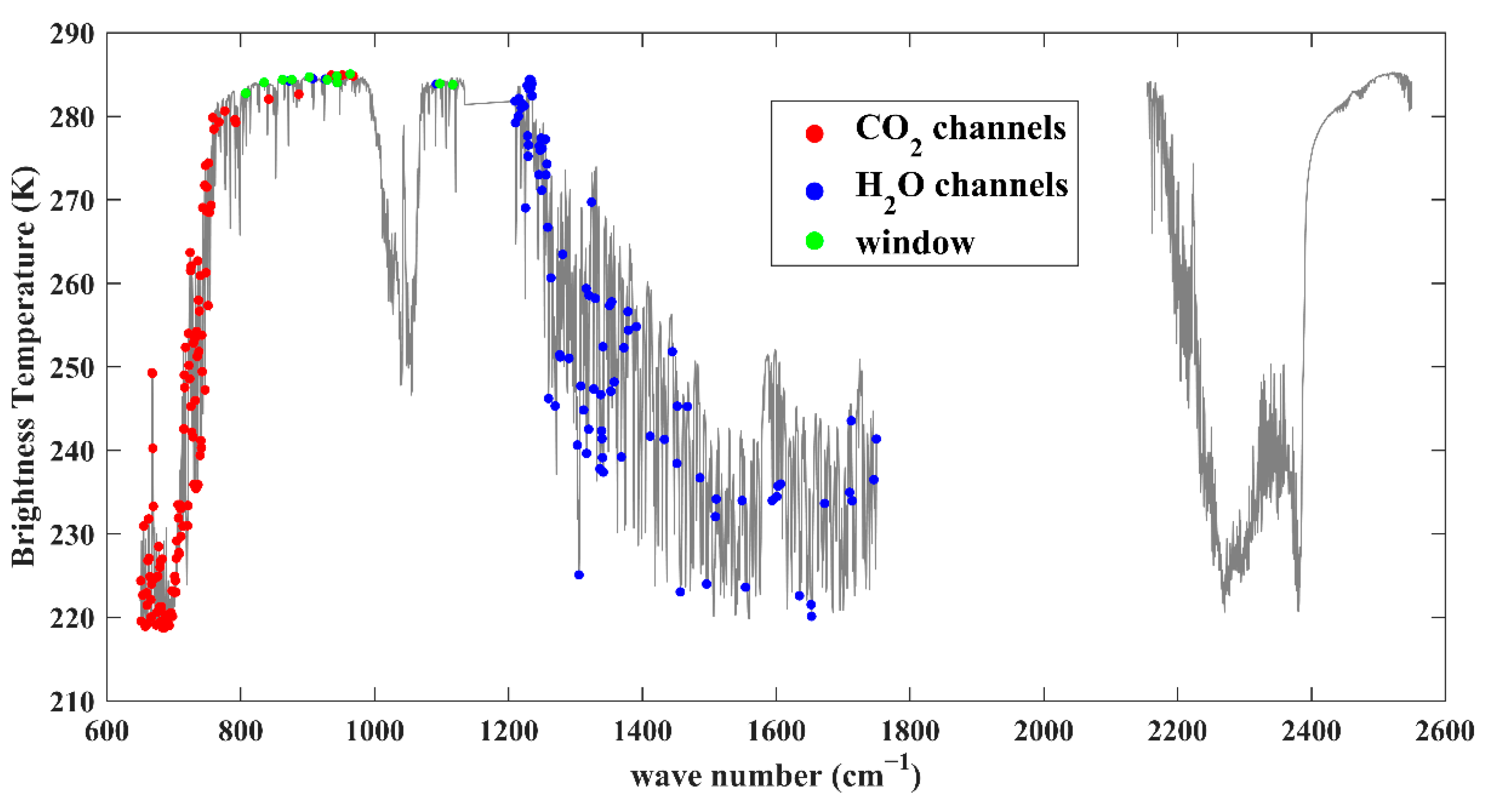
FengYun-3D/HIRAS collects spectral information in a total of 2287 channels. Although the infrared hyperspectral detector provides rich detection information, in practical applications, the use of all channels brings redundant information due to the correlation between channels. Since thousands of samples are needed to train the NNs, it is difficult to train the NNs with such a large quantity. Furthermore, it takes time computationally and the lower generalization performances make it difficult to get the best result. Therefore, it is necessary to select the channels that play a major role in the inversion. These selected channels can not only provide useful observation information, but also minimize the correlation between channels. In this experiment, the channel selection method of the principal component cumulative influence coefficient [31] has been adopted. The principal component cumulative influence coefficient method can not only obtain channels that preserve the most important information with greater influence and sensitivity, but also remove the correlation between channels. First of all, a fast radiative transfer model Radiative Transfer for TOVS(RTTOV) [32] was used to obtain the Jacobian matrix of CO2 and H2O absorption channels (CO2: 600–810 cm−1; H2O: 1210–1750 cm−1), which represent the sensitivity of brightness temperature of each channel to the atmospheric parameters. Then, the vertical pressure layer where the peak value of Jacobi matrix of CO2 and H2O absorption channels respectively was calculated. Finally, for the channels with the same pressure layer where the peak value is, channels with greater influence coefficient on the principal component were selected by using the method of cumulative influence coefficient of principal component. Through this method, 114 and 94 channels were finally selected between CO2 and H2O absorption channels, respectively. Considering the retrieval of the near-surface atmospheric temperature, 11 window channels have been added with reference to the window channels in IASI 300 channels [33]. The distribution of selected channels is shown in Figure 2. Considering that the water vapor absorption channels also contain the vertical distribution information of temperature, and the relative humidity is not only related to the atmospheric water vapor content, but also related to the atmospheric temperature, so we used all selected channels (219) to retrieve the atmospheric temperature and relative humidity profiles.

2.3. Cloud-Screening

Due to the weak transmission of IR on cloud, the impact of cloud is severe [34,35] and as a result the cloud-affected pixels need to be removed. The L2 products (FengYun-3D/MERSI-II 5-min granule cloud amount) of the MERSI instrument which is mounted on the FengYun-3D satellite platform were used to determine whether the HIRAS observation pixel is affected by cloud [36,37,38]. Those products include 5 min granule cloud amount and high cloud amount. Total cloud amount refers to the ratio of the sum of radiation emitted by all cloud pixels to the sum of radiation emitted by all pixels in a given region. Overall, 0% means clear sky, and 100% means cloudy sky. These products are orbit products with spatial resolution about 5 km.
First, the instruments to be matched were required to be divided into a master instrument (HIRAS) and a slave instrument (MERSI). In this study, the resolution of the main instrument’s sub-satellite point is 16 km. Because the FOV of the detector is often not circular (except for the sub-satellite point), in order to ensure the pixels are not polluted by cloud, all MERSI data points falling in a circle centered on the HIRAS observation pixel with a radius of 16 km are selected. The reciprocal of distance from these selected points to the center of the HIRAS pixel was used as their weight. If the data point of the slave instrument is located at the edge of the master instrument, it is given a smaller weight. The total cloud amount of the HIRAS’ pixel is the result of multiplying the cloud amount of these selected MERSI-II points by their corresponding weights and summing them up. Pixels with total cloud amount less than 5% were considered as cloudless.
In the present study, a scene of HIRAS sweeping past the Arctic region at 11:50 UTC on 2 August 2019 was selected. Figure 3a shows the brightness temperature distribution in window channel (wavenumber 900 cm−1). Lower brightness temperature indicates clouds presence (higher clouds). Areas with higher brightness temperature often give ground (clear sky) information, meaning that it may be the surface or mixture of mid-to-low layer cloud (partial cloudy). Red dots are the cloudless pixels of HIRAS selected by this technique. As can be observed, most of the selected clear sky pixels are on the ocean. For further verification, Figure 3b is the MERSI-II cloud amount distribution at the same time. The closer the color to yellow, the higher the cloud amount is, and the closer the color to blue, the lower the cloud amount is. By comparing these two pictures, the selected clear sky pixels are distributed in the area with very little cloud cover in Figure 3b, suggesting that the method produces promising results.

2.4. BP NN-Based Inversion of Atmospheric Temperature and Humidity Algorithm

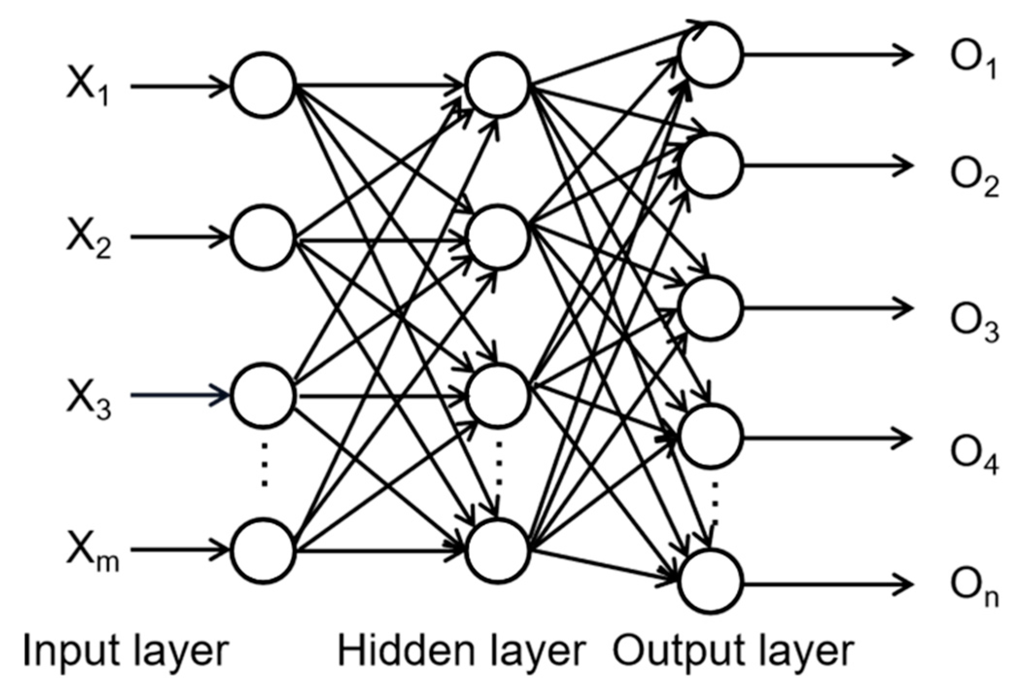
A NN is a non-linear, adaptive information processing system composed of a large number of nodes (neurons) and interconnections [39,40]. Each node represents a specific output function, called an activation function. Each connection between two nodes corresponds to a weighted value for the signal passing through the connection called a “weight”. The network output is different according to the connection mode of the network, the weight value and the excitation function. There are many NN models. Back Propagation (BP) NN is one of the most widely used NN models. It sends a series of inputs to the hidden layer after being weighted by the connection weight. After the neurons in the hidden layer summarize all the inputs, they generate some response output through a transfer function, and then connect the weights to the output layer through the next layer. Various neurons in the output layer aggregate all inputs to produce a response output. Then compare its output with the expected output, if they tend to be the same or the difference is very small, it can be considered that this network has basically learned this problem. If the difference is relatively large or unsatisfactory, the error between the network output and the expected output is returned, and repeated training is learned by adjusting the weight of each connection until it can produce an output that approximates the true answer. NN technology has been widely used in ground-based and space-based remote sensing retrieval [41,42,43,44].

2.4.1. Construction of BP Neural Network

A fully-learned three-layer feed-forward NN can approximate any function. Figure 4 shows the feed-forward NN structure. The network can implement continuous function mapping with arbitrary precision. The output of the NN model can be shown that:
O = F 2 ( Y v + b 2 )
Y = F 1 ( X w + b 1 )
where O is the output of the network; Y is the output of the hidden layer, and is also the input of the output layer; v is the matrix of the connection weight coefficients from the hidden layer to the output layer, w is the matrix of the connection weight coefficients from the input layer to the hidden layer, v and w are a group of random numbers at the initial moment; b1 and b2 are the element bias value matrix of hidden layer and output layer, respectively; F is the non-linear function of the neuron, which can be set according to each layer and can be tangent.
The BP algorithm performance index is the mean square error (MSE). For each input sample, the network output is compared with the target output, and the algorithm will adjust the network parameters to minimize the mean square error.
MSE = E [ e 2 ] = E [ ( t o ) 2 ]
where t is the expected output, o is the actual output, and e is the absolute error. In order to quantitatively analyze the advantages and disadvantages of the network, in addition to MSE, the correlation coefficient R, root mean square error (RMSE) and mean error (ME) between the inversion value and the actual value are also considered, expressed as:
R = i = 1 n ( x i x ¯ ) ( y i   y ¯ ) i = 1 n ( x i   x ¯ ) 2 i = 1 n ( y i   y ¯ ) 2 = i = 1 n x i y i n   x ¯   y ¯ ( i = 1 n x i 2 n   x ¯ 2 ) ( i = 1 n x i 2 n   x ¯ 2 )
RMSE = MSE
ME = i = 1 n x i y i n
where n represents the profiles number; xi is the atmospheric parameters retrieved from BP artificial NNs; yi is the actual atmospheric profile.

2.4.2. Network Topology

For temperature and relative humidity retrieval, 219 channels were used as an input to the NNs. Considering the radiation is also related to the zenith angle observed by the sensor, the sensor zenith angle was also used as the input of the NNs. The output layer of the NNs has 42 nodes, which represent 42 vertical atmospheric layers from 1–1000 hPa. The optimal number of hidden layer nodes determines the performance of the NNs. If the number of hidden layer nodes is too small, the network learning information processing ability will be reduced. However, too many hidden layer nodes will not only greatly increase the complexity of the network structure, but also slow down network learning speed. According to the Kolmogorov theorem and relevant literature [45], Equations (7) and (8) were used. They are as follows:
N h i d d e n = 2 N i n + 1 ,
N h i d d e n = N i n + ( N o u t , N c ) m a x 2 ,
where Nin and Nout represent the number of input and output neurons of the neural network, respectively. Nhidden represents the number of neurons in the hidden layer. NC represents the number of target classifications, and (Nout, Nc)max denotes the maximum value of Nout and NC. In the study, there is no such variable as Nc, so the value of the (Nout, Nc)max is determined as Nout. According to the above two formulas, numerous experiments were implemented in this study to optimize the NNs. Considering various factors such as calculation time and accuracy, finally 300 nodes were used for temperature and relative humidity retrieval.

2.4.3. Transfer Functions and Training Algorithms

In the NNs, the hyperbolic tangent S-type transfer function tansig was selected, as this function can express the non-linear relationship between nodes and is not affected by the size of the input value, and its output value is defined between −1 and 1. Due to the large number of training samples, more network parameters and a large amount of data storage, conjugate gradient algorithm: trainscg was used. The algorithm converges quickly and has stable performance, which is especially suitable for large-scale networks.

3. Retrieval Performance as Compared to ERA5

3.1. Inversion Results of Temperature and RH over Land

3.1.1. Validation of NNs with ERA5

Analysis of the temperature inversion results was from the bottom layer 1000 hPa to the upper layer 1 hPa (42 layers). Since water vapor is basically concentrated in the troposphere, and the relative humidity of water vapor above 100 hPa in the Arctic region decreases sharply to less than 1%. Therefore, relative humidity retrieval accuracy was only performed between 100–1000 hPa (25 layers).The performance of the NNs was evaluated on the basis of Equations (4)–(6).
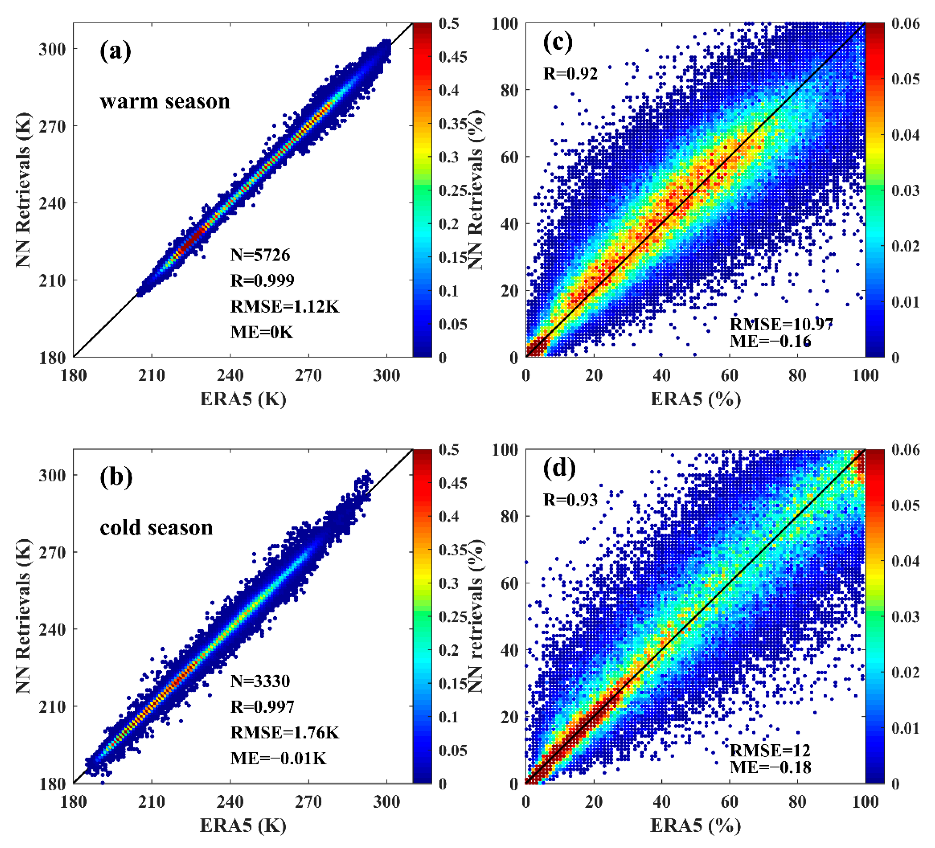
Figure 5 illustrates the density scatter diagram of retrieval results in two seasons. The high density values in red show where most of the data is located. From Figure 5a,b, it can be observed that although there are some retrieval results deviates slightly from the target temperature, these data points account for a very small proportion of all retrievals, most of the data points are concentrated on the line “Y=X”. In addition, as can be seen, correlation coefficients of retrieved temperature and target temperature in two seasons are basically above 0.99. Notably, the RMSE of retrieved temperature versus ERA5 in cold season (reported as 1.76 K) is 0.64 K larger than that of the warm season (reported as 1.12 K). The ME of temperature retrieval is basically around 0 K in two seasons. Figure 5c,d shows that, compared with the temperature validation, the results of RH are more scattered. The RMSE in warm and clod season is 10.97% and 12%, respectively. The ME of the RH inversions is basically around 0.

3.1.2. RMSE and ME Variation with Height

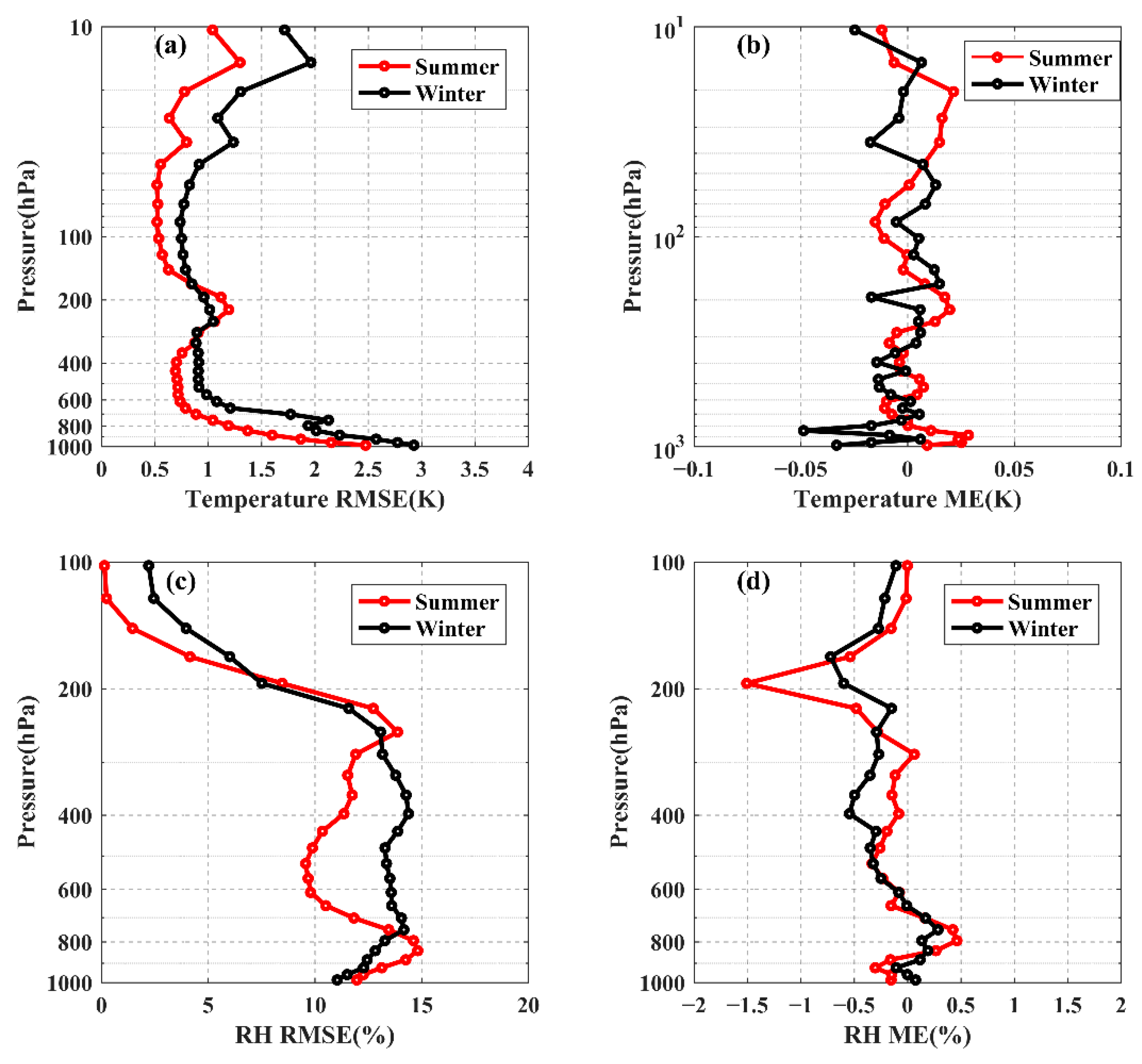
The RMSE and ME of retrieved temperature profiles between 10–1000 hPa on land is illustrated in Figure 6a,b. It can be observed that the RMSE curves in the two seasons are consistent, among which the accuracy of retrieved profiles in warm season is higher. The RMSE of temperature is generally within 1 K between 600 and 300 hPa in warm and cold season. It is worth noting that the accuracy of NNs is slightly lower in the near-surface layer than in other layers. This may be due to multiple energy exchanges between the lower atmosphere and the surface. The lower layer atmosphere will be affected by surface temperature, surface pressure, altitude and so on. Due to strong radiative cooling, there is a near-surface temperature inversion in the polar region, and the frequency is higher and the temperature inversion layer is thicker in cold season [46]. As a result, the RMSE of temperature in the lower level is greater in cold period, whose RMSE can reach 3 K near 1000 hPa. In the stratosphere, the RMSE in warm season is basically within 1.5 K, the RMSE in cold season can reach 2 K. The ME of temperature is between −0.05 and 0.05 K at each level.
As can be observed from Figure 6c, RMSE of RH is between 10% and 15% in the whole atmosphere, and the accuracy of RH is noticeably lower in cold season between 300–800 hPa. ME of RH is basically within the −0.5–0.5% range, except for the large deviation at 200 hPa (about −1.5%).

3.2. Inversion Results of Temperature and RH over Ocean

3.2.1. Validation of NNs with ERA5

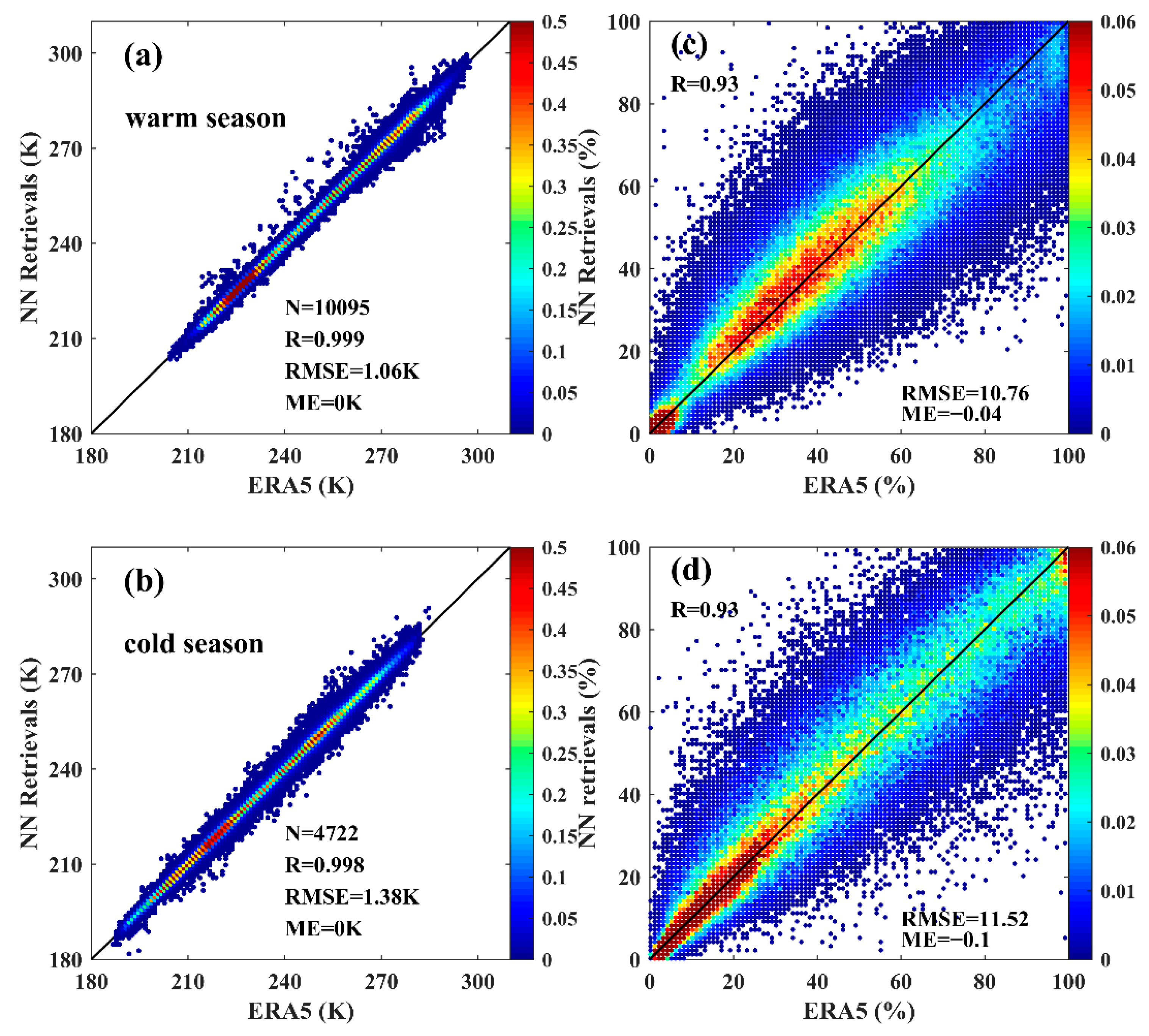
The retrieval results on ocean are summarized in Figure 7, where the left column depicts the density scatter diagram of temperature retrievals. Correlation coefficient between the temperature retrievals and ERA5 is above 0.99 in both warm and cold season. RMSE of temperature retrievals is 1.06 K and 1.38 K in the warm and clod season, respectively. The mean bias is also reasonable (0 K). In overall, temperature retrieval accuracy on ocean is higher than that on land. From the right column of Figure 7, it can be also concluded that there are more data points deviating from the line “Y=X” than temperature. Correlation coefficients of the two seasons are 0.93. The RMSE of the RH results on ocean is not significantly different from that on the land and is basically around 11%. The ME of RH retrievals is less than 0%, which suggests that RH retrieved from the NNs is slightly less than ERA5.

3.2.2. RMSE and ME Variation with Height

The RMSE and ME of retrieved peofiles between 10–1000 hPa on ocean is illustrated in Figure 8. Contrary to land cases, accuracy of temperature profiles retrieved from NNs in cold season is higher below 800 hPa. In the upper troposphere, RMSE of temperature in warm and cold season is basically within 1 K. In the stratosphere, retrieval accuracy in cold season is also lower, but RMSE can also be within 2.5 K. The absolute of ME is basically within 0.05 K. RMSE of RH in cold season is still larger than that in warm season, but their RMSE is generally maintained between 10% and 15%, whereas ME is within the −0.5–0.5% range.

4. Comparison of Retrieved Results to the Radiosonde Observation

Figure 9 shows RMSE and ME of temperature and RH profiles retrieved from NNs at different layers, with respect to RAOBs on land. Comparing the red and blue lines in Figure 9, we can draw the conclusion that the RMSE of profiles is generally slightly greater in the RAOB comparisons than in the ERA5 comparisons, but their behavior is consistent. From Figure 9a,b, it can be concluded that the RMSE of retrieved temperature profiles versus RAOBs is larger at about 1000 hPa and RMSE decreases rapidly with height. Performance of NNs versus RAOBs on land in warm season is higher than that in cold season, and RMSE can be within 1.5 K between 350–800 hPa. RMSE of temperature from 25 atmospheric vertical layers up to 50 hPa in warm season is 0.35 K lower than that in cold season in the RAOB comparisons.
As can be observed from Figure 9c,d, the RMSE of relative humidity profiles is also larger in the RAOB comparisons. RMSE of the relative humidity retrieved by the NNs is basically around 20% in the troposphere below 350 hPa. However, at 250 hPa, the inversion accuracy has decreased. It is about 30% in warm season and 22% in cold season.

5. Comparison between HIRAS Retrievals and AIRS Retrievals

5.1. Temperature

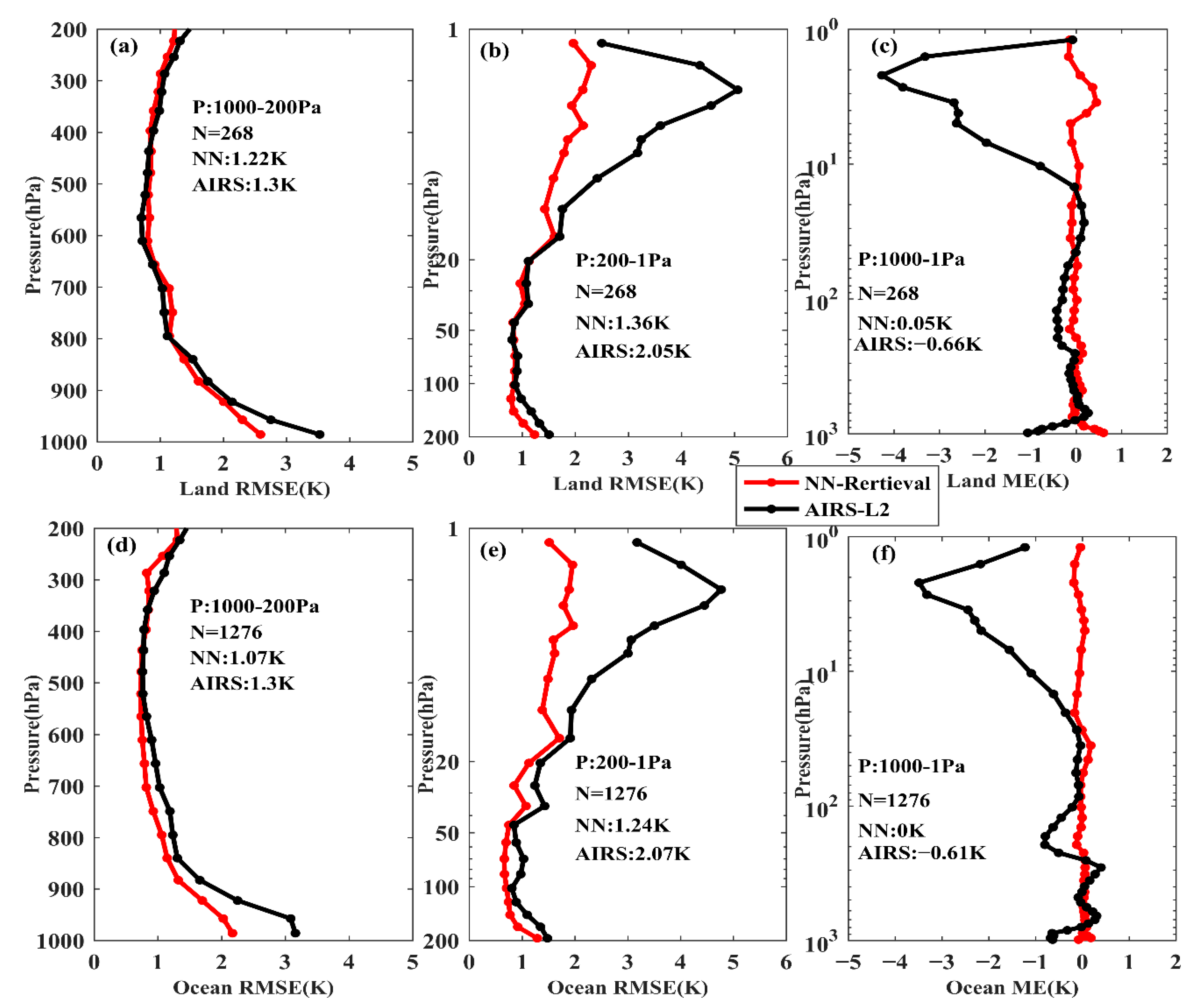
In order to further evaluate the performance of the proposed NNs in this study, we also compared the accuracy of retrievals using NN algorithm from HIRAS observations with AIRS L2 products (from May 2019 to April 2020, monthly 1, 10, 20, 30; using the same reference: ERA5). The AIRS L2 products were collected with ERA5 based on the critical of within 1 h in time and within 100 km in space. 268 samples (out of testing data) were collected on land and 1276 samples (out of testing data) were collected on ocean. AIRS products were linearly interpolated to the retrieval pressure layers and the results are illustrated in Figure 10. As shown, compared with ERA5, RMSE of retrieved temperature by NNs is consistent with that of AIRS products on land and ocean. Figure 10a,d in particular clearly show that NNs retrieval accuracy is comparable to AIRS temperature products in the upper troposphere and higher than AIRS products in the lower troposphere on land and ocean. The center column in Figure 10 clearly shows that the accuracy of temperature retrieved from HIRAS using NN algorithm is significantly better than that of AIRS products above 20 hPa. From the right column of Figure 10, we find that AIRS temperature products are significantly 4 K smaller than ERA5 above 20 hPa.

5.2. Relative Humidity

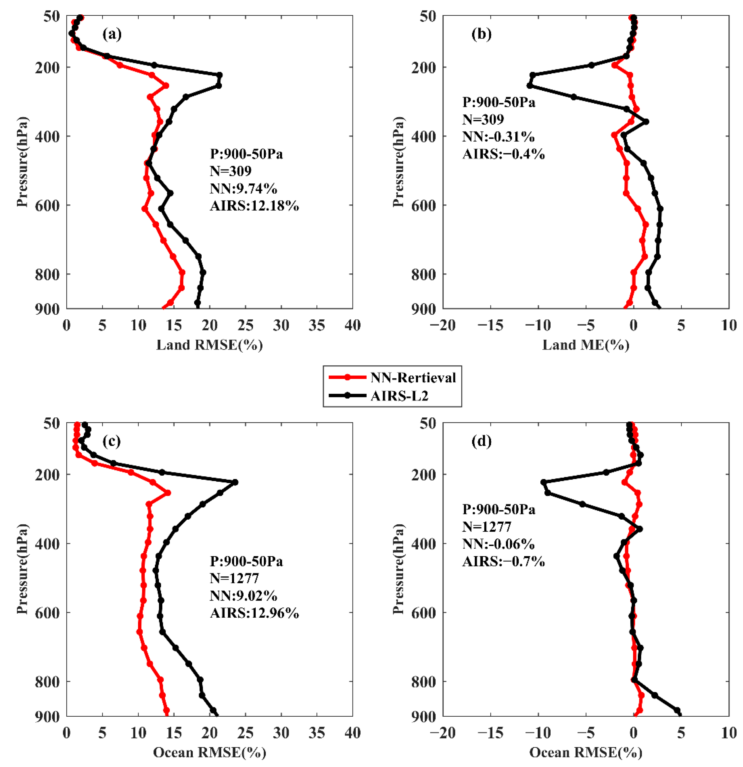
Taking ERA5 as a reference, we further compared the relative humidity retrievals obtained by NNs from HIRAS with AIRS products. Considering that most of the AIRS relative humidity products below 950 hPa are filled values, and the pressure layer is only up to 50 hPa, the results comparison was performed between 50–900 hPa. 309 and 1277 samples (out of test data) were collected on land and ocean, respectively. The results are illustrated in Figure 11. As can be observed, RMSE of RH profiles retrieved by NNs is also consistent with that of AIRS products both on land and ocean, but the RMSE of RH retrieved from NNs is lower than that of AIRS products from 50–900 hPa atmospheric vertical layers. There is a peak at about 250 hPa, but the RMSE and ME of the AIRS products is larger than that of the NNs retrievals.

6. Discussion

Our work proves the potential value of using the NN algorithm to retrieve temperature and RH profiles in the Arctic region under clear-sky condition. The NN algorithm not only avoids the complicated calculation process adopted in physically-based methods, but also obtains considerable accuracy. The proposed scheme only needs as input Fengyun-3D/HIRAS observations into the neural networks established in advance to realize the real-time retrieval of atmospheric temperature and RH profiles in the Arctic region. The dataset specially constructed from the region north of 60°Ncan better represent the climate conditions in the Arctic region, which is conducive to improving the learning ability of the neural networks and thus improving the retrieval accuracy of the NNs. The NNs were established according to the surface type and seasons, respectively. This can not only make the training samples of different models more representative, but also reduces the training difficulty of the neural networks [47]. Although we have improved the accuracy of the NN algorithm by dividing different types of samples, the errors of NNs retrievals still comes from the following aspects:
  • The algorithm parameter settings have affected our results, such as the number of hidden layer nodes. Even though we have done a lot of experiments, these parameters may not necessarily conform to the optimal parameter scheme.
  • Due to the topographic heterogeneity and elevation difference over the Arctic area, the performance of NNs established on land is slightly worse that on ocean.
  • The performance of the established NNs is also affected by the accuracy of the L2 cloud products in the polar region. Cloud-clearing is much more difficult on land than ocean, so there may be more samples polluted by cloud on land than ocean.
  • It is worth noting that the accuracy of NNs in the near-surface layer than in other layers. This may be due to multiple energy exchanges between the lower atmosphere and the surface. The lower layer atmosphere will be affected by the difference in surface temperature, surface pressure and so on.
  • As the fact that the ERA5 from ECMWF and the RAOBs exist certain deviation [48], and this deviation was also brought into retrievals, which resulting that RMSE of NN retrievals is larger than that of ERA5, when compared with RAOBs on land.

7. Conclusions

In this study, a new technique based on the NN algorithm was proposed for retrieving atmospheric parameters of the Arctic region (north of 60°N) under clear-sky from Fengyun-3D/HIRAS observations. Temperature and relative humidity profiles retrieved from the NNs were not only compared with the ERA5, but also compared with the conventional radiosonde profiles on land that can represent the true state of the atmosphere to further prove the significance of our research. Furthermore, we also compared our retrievals with AIRS L2 products. The results of our work can be summarized as follows:
  • The performance of temperature retrieval in warm season is better than that in cold season, and the accuracy of temperature retrievalon ocean is higher than that on land. Compared with ERA5 on land, RMSE of temperature from 42 vertical layers is 1.12 K in warm season, and 1.76 K in cold season. Compared with ERA5 on ocean, the RMSE of temperature retrieved on warm and cold season is 1.06 K and 1.38 K, respectively. RMSE of retrieved RH profiles during the whole period is between 10% and 15% both on land and ocean.
  • The influence of surface parameters and the existence of near-surface inversion layers in the Arctic region make the accuracy in the near-surface layer unsatisfactory. Compares with ERA5 on land, RMSE of warm season at about 1000 hPa is 2.5 K, and the RMSE in cold season can reach 3 K.
  • RMSE of retrieved profiles from NNs on land compared with collocated RAOBs is slightly higher. While direct comparison with different data sets is not available, but the errors of retrieval profiles still vary within a reasonable range.
  • NNs can achieve comparable performance in upper troposphere, and better performance below 900 hPa when compared with AIRS L2 products. This advantage is even more pronounced in the stratosphere.
All in all, the present study proposed the retrievals of temperature and relative humidity profiles in real-time from the FengYun-3D/HIRAS observation data, and the errors of the retrievals were also within a reasonable range, compared with ERA5, RAOB and AIRS L2 products. This is of great significance for the study of climate in the Arctic region, because it can not only make up for the 5 days latency of ERA5 in time, but also overcome the difficulty of obtaining profiles from radiosondes due to sparse distribution. The method we proposed has great prospects in operational implementation in the future. By analyzing the error sources of the neural networks mentioned in the Discussion section, cloud and complex surface parameters can both affect the performance of NNs, so possible directions of future work include: (1) Explore the use of multiple remote sensing fusions (such as MWTS, MWHS carried onboard FengYun-3D) to reduce the influence of cloud-clearing errors on the retrieval results, (2) Increase the surface constraint information (e.g., surface elevation data, surface temperature and surface pressure) to improve the near-surface retrieval accuracy.

Author Contributions

Conceptualization, J.H. and Y.B.; methodology, J.H., Y.B., J.L., H.L. and G.P.P.; software, J.H. and X.C.; validation, J.L., H.L. and L.Z.; formal analysis, Y.B., G.P.P. and P.K.; investigation, J.H.; resources, J.L. and H.L.; data curation, J.H.; writing—original draft preparation, J.H., Y.B. and H.L.; writing—review and editing, J.H., Y.B. and G.P.P.; visualization, L.Z.; supervision, Y.B.; project administration, J.L. and H.L.; funding acquisition, Y.B., and J.L. All authors have read and agreed to the published version of the manuscript.

Funding

This study was supported by the National Key Research and Development Program of China (2018YFC1407204, 2018YFC1407200, 2017YFB0502800, 2017YFC1501704), Graduate Research and Innovation Program in Jiangsu Province (KYCX20_0953), and National Natural Science Foundation of China (41975046). G.P.P.’s participation was supported financially by the European Union’s Horizon 2020 Marie Skłodowska-Curie Project “ENViSIoN-EO” (grant agreement No 752094).

Institutional Review Board Statement

Not applicable.

Informed Consent Statement

Not applicable.

Data Availability Statement

All data generated or analyzed during this study are included in this article.

Acknowledgments

The numerical calculations in this paper have been done on the supercomputing system in the Supercomputing Center of Nanjing University of Information Science & Technology. We thank the National Satellite Meteorological Center for providing the satellite data, which were obtained on this website (http://satellite.nsmc.org.cn/PortalSite/Data /Satellite.aspx, accessed on 1 May 2019 to 30 April 2020), and the ECMWF for providing ERA5 reanalysis data used here (https://cds.climate.copernicus.eu/#!/search?text=ERA5&type=dataset, accessed on 1 May 2019 to 30 April 2020). Last but not least, we appreciate the sounding data that provided by University of Wyoming, and this data can be archived online (http://weather.uwyo.edu/upperair/sounding.html, accessed on 1 May 2019 to 30 April 2020).

Conflicts of Interest

The authors declare no conflict of interest.

References

  1. Zhao, J.; Zhong, W.; Diao, Y.; Cao, Y. The Rapidly Changing Arctic and Its Impact on Global Climate. J. Ocean. Univ. China 2019, 18, 537–541. [Google Scholar] [CrossRef]
  2. Francis, J.A.; Vavrus, S.J. Evidence linking Arctic amplification to extreme weather in mid-latitudes. Geophys. Res. Lett. 2012, 39, 1–6. [Google Scholar] [CrossRef]
  3. Ghatak, D.; Frei, A.; Gong, G.; Stroeve, J.; Robinson, D. On the emergence of an Arctic amplification signal in terrestrial Arctic snow extent. J. Geophys. Res. Atmos. 2010, 115, 1–8. [Google Scholar] [CrossRef] [Green Version]
  4. Lei, G. Uncertainty of Temperature Variability in the Arctic of the 20th Century. J. Subtrop. Resour. Environ. 2012, 7, 34–39. [Google Scholar]
  5. Wu, B. Progresses in the Impact Study of Arctic Sea Ice Loss on Wintertime Weather and Climate Variability over East Asia and Key Academic Disputes. Chin. J. Atmos. Sci. 2018, 42, 786–805. [Google Scholar] [CrossRef]
  6. Hu, X.; Cai, M.; Yang, S.; Sejas, S.A. Air temperature feedback and its contribution to global warming. Sci. China Earth Sci. 2018, 61, 1491–1509. [Google Scholar] [CrossRef]
  7. Schneider, E.K.; Kirtman, B.P.; Lindzen, R.S. Tropospheric Water Vapor and Climate Sensitivity. J. Atmos. Sci. 1999, 56, 1649–1658. [Google Scholar] [CrossRef]
  8. Zhao, T.; Tu, K.; Yan, Z. Advances of Atmospheric Water Vapor Change and Its Feedback Effect. Progress. Inquisitiones DE Mutat. Clim. 2013, 9, 79–88. [Google Scholar] [CrossRef]
  9. Li, H.; Shu, R.; Xue, Y. Pushbroom Hyperspectral Imager And Its Potential Application To Oceanographic Remote Sensing. J. Infrared Millim. Waves 2002, 21, 429–433. [Google Scholar]
  10. Shukla, A.; Kot, R. An Overview of Hyperspectral Remote Sensing and its applications in various Disciplines. IRA Int. J. Appl. Sci. 2016, 5, 85. [Google Scholar] [CrossRef] [Green Version]
  11. Staenz, K.; Held, A. Summary of current and future terrestrial civilian hyperspectralspaceborne systems. Int. Geosci. Remote Sens. Symp. 2012, 123–126. [Google Scholar] [CrossRef]
  12. Zhang, C.; Mu, T.; Yan, T.; Chen, Z. Overview of Hyperspectral Remote Sensing Technology. Spacecr. Recover. Sens. 2018, 39, 104–114. [Google Scholar] [CrossRef]
  13. Wang, C.; Du, M.; Xie, X.; Li, X.; Li, B. Atmospheric Temperature and Hunidity Profiles Physical Rertieval Algorithm for Satellite-Borne Microwave Sensors. Aerosp. Shang Hai 2018, 35, 73–80. [Google Scholar]
  14. Guan, Y.; Ren, J.; Bao, Y.; Lu, Q.; Liu, H.; Xiao, X. Research of the infrared high spectral( IASI) satellite remote sensing at- mospheric temperature and humidity profiles based on the one- dimensional variational algorithm. Trans. Atmos. Sci. 2019, 42, 602–611. [Google Scholar]
  15. Guan, L. Retrieving Atmospheric Profiles from MODIS/AIRS Observations I.Eigenvector Regression Algorithms. J. Nanjing Inst. Meteorol. 2006, 29, 756–761. [Google Scholar]
  16. Jiang, D.; Dong, C.; Wei, W. Preliminary Study on the Capacity of High Spectral Resolution Infrared Atmospheric Sounding Instrument Using AIRS Measurements. J. Remote Sens. 2006, 10, 586–592. [Google Scholar]
  17. Liu, H.; Dong, C.; Zhang, W.; Zhang, P. Retrieval of clear-air atmospheric temperature profiles using AIRS observations. Acta Meteorol. Sin. 2008, 66, 513–519. [Google Scholar]
  18. Bao, Y.; Cai, X.; Qian, C.; Min, J.; Lu, Q.; Zuo, Q. 0–10 Km Temperature and Humidity Profiles Retrieval From Ground-Based Microwave Radiometer. J. Trop. Meteorol. 2018, 24, 223–252. [Google Scholar]
  19. Blackwell, W.J. A neural-network technique for the retrieval of atmospheric temperature and moisture profiles from high spectral resolution sounding data. IEEE Trans. Geosci. Remote Sens. 2005, 43, 2535–2546. [Google Scholar] [CrossRef]
  20. Cai, X.; Bao, Y.; Petropoulos, G.P.; Lu, F.; Lu, Q.; Zhu, L.; Wu, Y. Temperature and humidity profile retrieval from FY4-GIIRS hyperspectral data using artificial neural networks. Remote Sens. 2020, 12, 1872. [Google Scholar] [CrossRef]
  21. Guan, L.; Liu, Y.; Zhang, X. Application of Artificial Neural Network Algorithm in Retrieving Atmospheric Temperature Profiles from Hyperspectral Infrared Data. Trans. Atmos. Sci. 2010, 33, 341–346. [Google Scholar]
  22. Lerner, J.A.; Weisz, E.; Kirchengast, G. Temperature and humidity retrieval from simulated Infrared Atmospheric Sounding Interferometer (IASI ) measurements. J. Geophys. Res. Atmos. 2002, 107, ACH-4. [Google Scholar] [CrossRef] [Green Version]
  23. Milstein, A.B.; Blackwell, W.J. Neural network temperature and moisture retrieval algorithm validation for AIRS/AMSU and CrIS/ATMS. J. Geophys. Res. Atmos. 2016, 121, 1414–1430. [Google Scholar] [CrossRef] [Green Version]
  24. Zhang, X.; Guan, L.; Wang, Z.; Han, J. Retrieval Atmospheric Temperature Profiles Using Artificial Neural Network Approach. Meteorol. Mon. 2009, 35, 137–142. [Google Scholar]
  25. Huang, X.; Zhang, X.; Leng, L.; Li, F.; Fan, Y. Study on retrieval method with MonoRTM for microwave radiometer measurements. J. Meteorol. Sci. 2013, 33, 138–145. [Google Scholar]
  26. Deng, K.A.K.; Lamine, S.; Pavlides, A.; Petropoulos, G.P.; Srivastava, P.K.; Bao, Y.; Hristopulos, D.; Anagnostopoulos, V. Operational Soil Moisture from ASCAT in Support of Water Resources Management. Remote Sens. 2019, 11, 579. [Google Scholar] [CrossRef] [Green Version]
  27. Deng, K.A.K.; Lamine, S.; Pavlides, A.; Petropoulos, G.P.; Bao, Y.; Srivastava, P.K.; Guan, Y. Large scale operational soil moisture mapping from passive MW radiometry: SMOS product evaluation in Europe & USA. Int. J. Appl. Earth Obs. Geoinf. 2019, 80, 206–217. [Google Scholar] [CrossRef]
  28. Yang, J.; Zhang, P.; Lu, N.; Yang, Z.; Shi, J.; Dong, C. Improvements on global meteorological observations from the current Fengyun 3 satellites and beyond. Int. J. Digit. Earth 2012, 5, 251–265. [Google Scholar] [CrossRef]
  29. Wu, C.; Qi, C.; Hu, X.; Gu, M.; Yang, T.; Xu, H.; Lee, L.; Yang, Z.; Zhang, P. FY-3D HIRAS Radiometric Calibration and Accuracy Assessment. IEEE Trans. Geosci. Remote Sens. 2020, 58, 3965–3976. [Google Scholar] [CrossRef]
  30. Divakarla, M.G.; Barnet, C.D.; Goldberg, M.D.; McMillin, L.M.; Maddy, E.; Wolf, W.; Zhou, L.; Liu, X. Validation of Atmospheric Infrared Sounder temperature and water vapor retrievals with matched radiosonde measurements and forecasts. J. Geophys. Res. Atmos. 2006, 111, 1–20. [Google Scholar] [CrossRef] [Green Version]
  31. Zhang, J.; Wang, G.; Zhang, H.; Huang, J.; Chen, J.; Wu, L. Experiment on hyperspectral atmospheric infrared sounder channel selection based on the cumulative effect coefficient of principal component. Trans. Atmos. Sci. 2011, 34, 36–42. [Google Scholar]
  32. Liu, L.; Li, Y. The application and Research Advances of RTTOV Fast Radiative Transfer Mode. J. Anhui Agri. Sci. 2016, 44, 230–232. [Google Scholar] [CrossRef]
  33. Collard, A.D. Selection of IASI channels for use in numerical weather prediction. Q. J. R. Meteorol. Soc. 2007, 133, 177–1991. [Google Scholar] [CrossRef]
  34. Ackerman, S.A.; Strabala, K.I.; Menzel, W.P.; Frey, R.A.; Moeller, C.C.; Gumley, L.E. Discriminating clear sky from clouds with MODIS. J. Geophys. Res. Atmos. 1998, 103, 32141–32157. [Google Scholar] [CrossRef]
  35. Cho, C.; Staelin, D.H. Cloud clearing of Atmospheric Infrared Sounder hyperspectral infrared radiances using stochastic methods. J. Geophys. Res. Atmos. 2006, 111, 1–10. [Google Scholar] [CrossRef] [Green Version]
  36. Guan, L.; Wang, Z. Objective Determination of AIRS Cloud Mask Using Co-located MODIS Cloud Mask. Sci. Meteorol. 2007, 57, 516–521. [Google Scholar]
  37. Lu, Q.; Zhou, F.; Qi, C.; Hu, X.; Xu, H.; Wu, C. Spectral performance evaluation of high-spectral resolution infrared atmospheric sounder onboard FY-3D. OptisPrecis. Eng. 2019, 27, 2105–2115. [Google Scholar] [CrossRef]
  38. Wang, L.; Tremblay, D.; Zhang, B.; Han, Y. Fast and accurate collocation of the visible infrared imaging radiometer suite measurements with Cross-track Infrared Sounder. Remote Sens. 2016, 8, 76. [Google Scholar] [CrossRef] [Green Version]
  39. Hecht-Nielsen, R. Theory of the backpropagation neural network. IEEE IJCNN 1989, 593–605. [Google Scholar] [CrossRef]
  40. Krasnopolsky, V.M. Neural network emulations for complex multidimensional geophysical mappings: Applications of neural network techniques to atmospheric and oceanic satellite retrievals and numerical modeling. Rev. Geophys. 2007, 45, 1–34. [Google Scholar] [CrossRef] [Green Version]
  41. Jiang, D.; Cao, S.; Qu, Y. A Neural network application to retrieval of atmosoheric temperature profile from high speatral resolution infrared measurements. J. Trop. Meteorol. 2010, 26, 819–824. [Google Scholar]
  42. Sai Gowtam, V.; Tulasi Ram, S. An Artificial Neural Network-Based Ionospheric Model to Predict NmF2 and hmF2 Using Long-Term Data Set of FORMOSAT-3/COSMIC Radio Occultation Observations: Preliminary Results. J. Geophys. Res. Sp. Phys. 2017, 122, 743. [Google Scholar] [CrossRef]
  43. Yang, Y.; Shen, F.; Yang, Z.; Feng, X. Prediction of Solar Wind Speed at 1 AU Using an Artificial Neural Network. Sp. Weather 2018, 16, 1227–1244. [Google Scholar] [CrossRef]
  44. Zheng, G.; Yang, J.; Li, X.; Zhou, L.; Ren, L.; Chen, P.; Zhang, H.; Lou, X. Using artificial neural network ensembles with crogging resampling technique to retrieve sea surface temperature from HY-2A scanning microwave radiometer data. IEEE Trans. Geosci. Remote Sens. 2019, 57, 985–1000. [Google Scholar] [CrossRef]
  45. Jiao, B.; Ye, M. Determination of Hidden Unit Number in a BP Neural Network. J. O Shanghai Dianji Univ. 2013, 16, 113–117. [Google Scholar]
  46. Cheng, G.; Gao, Z.; Zheng, Y.; Dai, C.; Zhou, M. A Study on Low-level Jets and Temperature Inversion over the Arctic Ocean by using SHEBA Data. Clim. Environ. Res. 2013, 18, 23–31. [Google Scholar] [CrossRef]
  47. Liu, Y.; Cai, B.; Ban, X.X. Research progress of retrieving atmospheric humidity profiles from AIRS data. Adv. Earth Sci. 2013, 28, 890–896. [Google Scholar]
  48. Keernik, H.; Jakobson, E. Evaluating reanalyses performance in the Baltic Sea region by using assimilated radiosonde data. Int. J. Climatol. 2018, 38, 1820–1832. [Google Scholar] [CrossRef]
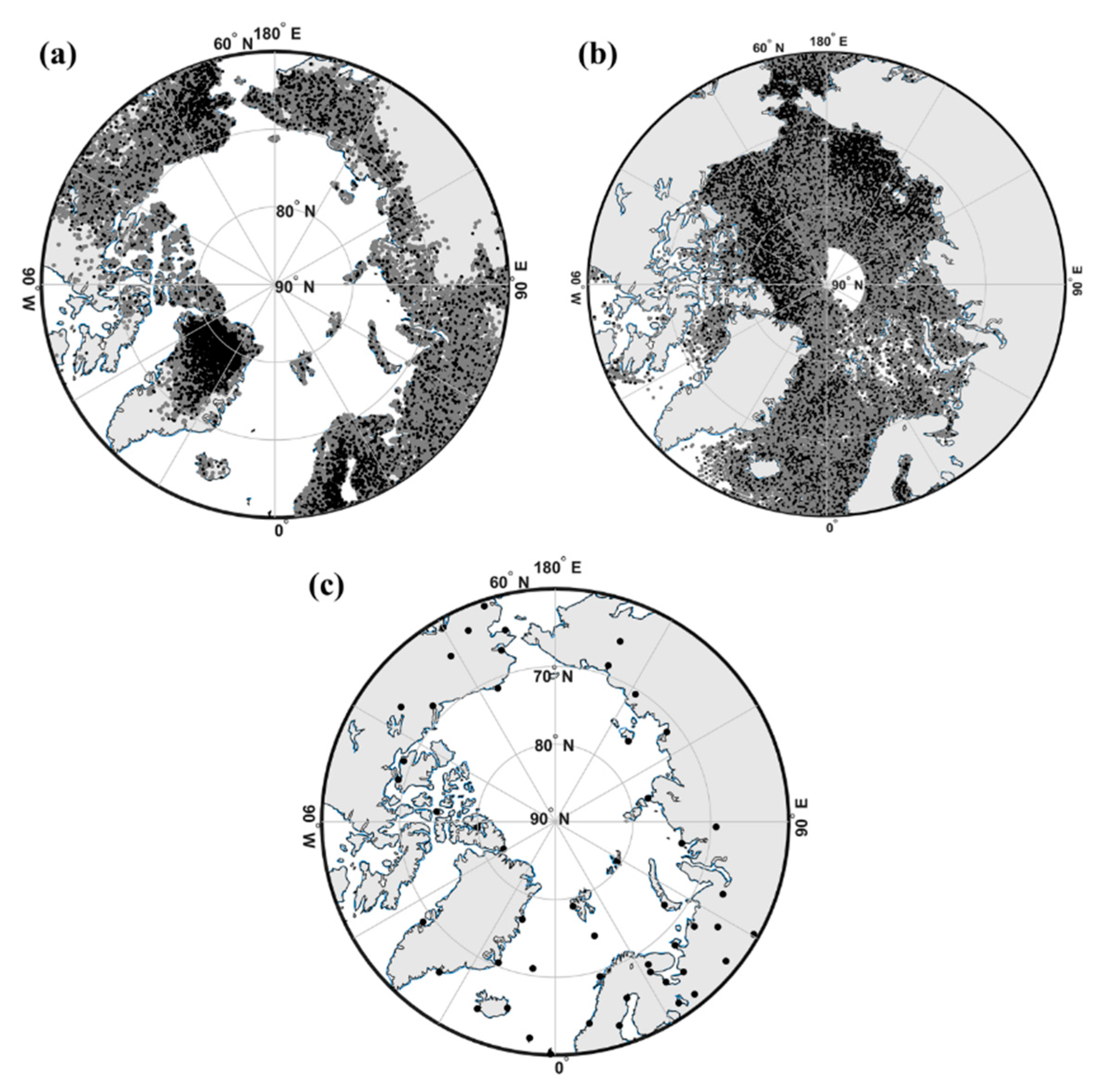
Figure 1. (a,b) Distribution of samples on land and ocean obtained under clear-sky conditions in the Arctic region, respectively. Gray solid points represent test samples; black solid points represent training samples. (c) Distribution of radiosonde stations in the arctic. The solid dots represent the radiosonde stations.
Remotesensing 13 01884 g001
Figure 2. Channels used in NNs retrieval. Red, blue and green dots represent channels selected in CO2, H2O and window band, respectively.
Remotesensing 13 01884 g002
Figure 3. (a) Clear sky pixels of HIRAS selected by matching FengYun-3D/MERSI-II 5-min granule cloud amount on 11:50 UTC, 2 August 2019. (b) An example of cloud amount distribution of L2 product from FengYun-3D/MERSI-II on 11:50 UTC, 2 August 2019.
Remotesensing 13 01884 g003
Figure 4. Three-layer Feed-forward Neural Network structure.
Remotesensing 13 01884 g004
Figure 5. Density scatter diagram of retrieval results on land; (a,b)The relationship between the temperature retrievals of all 42 atmospheric layers up to 1 hPa and ERA5. (c,d) The relationship between the RH retrievals of all the 25 atmospheric layers up to 100 hPa and ERA5 (N represents the number of validation samples; R represents the correlation coefficient).
Remotesensing 13 01884 g005
Figure 6. Profile retrieval errors for (a,b) temperature, (c,d) RH, with respect to ERA5 on land.
Remotesensing 13 01884 g006
Figure 7. Density scatter diagram of retrieval results on ocean; (a,b) The relationship between the temperature retrievals of all 42 atmospheric layers up to 1 hPa and ERA5. (c,d) The relationship between the RH retrievals of all the 25 atmospheric layers up to 100 hPa and ERA5 (N represents the number of validation samples; R represents the correlation coefficient).
Remotesensing 13 01884 g007
Figure 8. Profile retrieval errors for (a,b) temperature, (c,d) RH,with respect to ERA5 on ocean.
Remotesensing 13 01884 g008
Figure 9. Profile retrieval errors for (a,b) temperature, (c,d) RH, with respect to RAOBs. The red line represents the RMSE of NNs retrievals versus ERA5 and the blue line represents NNs retrievals versus collocated RAOBs.
Remotesensing 13 01884 g009
Figure 10. Accuracy comparisons between Aqua/AIRS-L2 temperature products and NNs retrievals versus ERA5. (ac) The RMSE and ME of the temperature on land, respectively. (df) The RMSE and ME of temperature on ocean, respectively. The red dotted line represents the comparison between the retrievals from NNs and ERA5 data, the black solid line represents the comparison between AIRS products and the ERA5 data.
Remotesensing 13 01884 g010
Figure 11. Accuracy comparisons between Aqua/AIRS-L2 RH products and NNs retrievals versus ERA5. (a,b) The RMSE and ME of RH on land, respectively; (c,d) the RMSE and ME of RH on ocean, respectively. The red dotted line represents the comparison between the retrievals from NNs and ERA5 data, the black solid line represents the comparison between AIRS products and the ERA5 data.
Remotesensing 13 01884 g011
Table 1. Spectral characteristic of Fengyun-3D/HIRAS channels.
Band NameSpectral Range (cm−1)Spectral Resolution (cm−1)Sensitivity(NE∆T@250K)
Long Wave650–1136 (15.38–8.8 μm)0.6250.15–0.4 K
Medium Wave 11210–1750 (8.26–5.71 μm)1.250.1–0.7 K
Medium Wave 22155–2550 (4.64–3.92 μm)2.50.3–1.2 K
Table 2. Data set for neural networks acquired under clear sky conditions in the Arctic.
SeasonLandOcean
warm27,39530,283
cold16,64823,607
Table 3. Number of Collocated RAOB Datasets.
SeasonT NumberRH Number
warm944938
cold353356
Table 4. Information of 51 radiosonde stations used in this study (Sta represents sounding station number, Lat represents latitude of the station, and Lon represents longitude of the station).
StaLatLonStaLatLonStaLatLon
70,20064.5−165.4371,08282.5−62.35236562.5317.45
70,13366.86−162.63422068.7−52.85102874.519
70,21960.78−161.84436065.6−37.63218565.5522.13
70,02671.28−156.79401863.96−22.622,21767.1532.35
70,23162.96−155.61433970.48−21.9522,00868.133.11
70,27361.16−150.01432076.76−18.6622,82061.8134.26
70,26164.81−147.88408965.28−14.422,52264.9534.65
71,95768.31−133.53100170.93−8.6622,84561.538.93
71,04365.28−126.75601162.01−6.7622,54364.6240.51
71,93469.03−111.93300560.13−1.1822,27167.8844.13
71,92569.13−105.06124163.719.6123,80261.6850.78
71,92474.7−94.97100478.9111.9320,74472.3652.7
71,91779.98−85.93101069.316.1323,20567.6353.03
23,41565.1257.120,04680.6158.0523,92160.6860.45
23,33066.5366.6620,67473.580.423,07869.3288.22
20,29277.71104.321,43276137.8625,42865.32160.23
21,82471.58128.9121,94670.61147.8825,12368.75161.28
Publisher’s Note: MDPI stays neutral with regard to jurisdictional claims in published maps and institutional affiliations.