Article

Analysis of the Response of Long-Term Vegetation Dynamics to Climate Variability Using the Pruned Exact Linear Time (PELT) Method and Disturbance Lag Model (DLM) Based on Remote Sensing Data: A Case Study in Guangdong Province (China)

1
School of Geography, South China Normal University, Guangzhou 510631, China
2
The Joint Laboratory of Plateau Surface Remote Sensing, Tibet University, Lhasa 850000, China
*
Author to whom correspondence should be addressed.
Remote Sens. 2021, 13(10), 1873; https://doi.org/10.3390/rs13101873
Submission received: 10 March 2021 / Revised: 14 April 2021 / Accepted: 7 May 2021 / Published: 11 May 2021
(This article belongs to the Section Environmental Remote Sensing)

Abstract

:
The dynamic change and spatial–temporal distribution of vegetation coverage are of great significance for regional ecological evolution, especially in the subtropics and tropics. Identifying the heterogeneity in vegetation activities and its response to climate factors is crucial for projecting ecosystem dynamics. We used long-term (2001–2018) satellite-derived enhanced vegetation index (EVI) datasets and climatic factors to analyze the spatiotemporal patterns of vegetation activities in an experimental area in Guangdong Province (China), as well as their links to changes in temperature (TEM), relative humidity (HUM), precipitation (PRE), sunshine duration (SUN), and surface runoff. The pruned exact linear time change point detection method (PELT) and the disturbance lag model (DLM) were used to understand the detailed ecological coverage status and time lag relationships between the EVI and climatic factors. The results indicate the following. (1) At the whole regional scale, a significant overall upward trend in the EVI variation was observed in 2001–2018. More specifically, there were two distinct periods with different trends, which were split by a turning point in 2005. PRE was the main climate-related driver of the rising EVI pre-2005, and the increase in TEM was the main climate factor influencing the forest EVI variation post-2006. (2) A three-month time lag effect was observed in the EVI response to relative humidity. The same phenomenon was found in the sunshine duration factor. (3) The EVI of farmlands (one type of land use) exhibited the largest lags between relative humidity and the sunshine duration factor, followed by grasslands and forests. (4) The comprehensive index of surface runoff could explain the time lags of vegetation activities, and the surface runoff value showed an apparently negative relationship with the vegetation coverage change.

1. Introduction

Vegetation plays an essential role in terrestrial ecosystems and is a dominant link between the atmosphere, soil, and biosphere with respect to the transfer of materials and exchange of energy [1]. Changes in vegetation differ significantly on a regional scale due to the considerable spatial and temporal heterogeneity of climate factors [2,3]. To understand the mechanisms behind the growth processes of vegetation ecosystems, it is necessary to monitor spatiotemporal changes and quantitatively assess the response of vegetation and associated feedbacks to the Earth’s climate system on regional and global scales. Consequently, many studies have been conducted in this field. For example, studies focusing on climate change have aimed to understand the relationship between vegetation growth and climate factors, such as temperature and precipitation, on inter-annual and intra-annual scales [4,5].
Climate extremes, such as drought, can also drive vegetation dynamics, and this is particularly true in regions with a widespread karst geomorphology, where the soil is not sufficiently water retentive [6]. It has been determined that climate change will cause an increase in vegetation coverage, and the growing season will be prolonged in affected regions. However, extreme climate events and human activities have degraded the vegetation cover [7,8]. Therefore, gaining an understanding of how terrestrial ecosystems respond to climate change in ecologically fragile regions would assist in developing sustainable adaptation strategies and policies for ecosystem management [9].
The most effective way to monitor and characterize land surface dynamics is to analyze long-term records of vegetation indices, such as the Enhanced Vegetation Index (EVI), which is functionally correlated with vegetation coverage derived from satellite remote sensing [10]. It can reduce the effect of the saturation problem present in the NDVI (Normalized Difference Vegetation Index), while remaining sensitive to canopy variations in high biomass conditions [11]. It has a stronger ability to reflect vegetation growth and vigor in high-coverage areas and has been used to model plant processes [12,13]. Many studies have used satellite observations to observe vegetation coverage trends and their relationships with climatic factors [8,9,14]. In this respect, previous studies have found that vegetation growth dynamics underwent a significantly positive increasing trend in Central and Southern China from 1982 to 2011 [15], and a positive correlation between temperature and vegetation was observed in the northeastern part of Guangdong Province [8]. However, studies focusing on the relationship between the variability in vegetation productivity and three climatic variables (air temperature, precipitation, and solar radiation) are scarce [3]. In this respect, Kong et al. [16] found that the length of the time lag varied between different land-cover types. Similarly, A et al. [17] found that precipitation had a monthly time-lag effect on vegetation growth in the agroecological zone. There is no doubt that the relationship between vegetation coverage and climatic factors shows a significant temporal and spatial heterogeneity. However, the study in [16] only used records of 15-day intervals of long-term vegetation indices, obtained from remote sensing and meteorological datasets, to estimate time lags, which may have introduced undesirable errors. In addition, the impact of time lags associated with cumulative climatic factors, which exhibit different lengths on the regional ecological boundary between tropical and subtropical regions, remains unclear.
The hilly ecological environment of Southern China is fragile and suffers from severe soil erosion [18]. In addition, changes in climate and surface runoff pose a severe threat to vegetation cover [19,20]. The study in [21] found that the soil erosion in South China is strongly dependent on the land use type, altitude, and slope. A recent study suggested that the daily temperature had increased substantially in Guangdong province over a recent 30-year period and that this has a positive correlation with the net primary productivity [22]. Wu et al. [23] reported that the decrease in the greenness of spring vegetation was significantly and positively affected by the temperature in Northern Guangdong from 2001 to 2013, and Yu et al. [24] reported that the summer precipitation has decreased in South China and that vegetation greening can minimize the risk of floods. The extreme drought of 2009/2010 in Southwestern China was the driest event in the past 50 years [25], and extreme rainfall and more frequent floods have shown increase trend in Southwest China [18]. All these studies show that climate variability has led to significant changes in vegetation, climate change (which is associated with an increase in precipitation), extreme floods, and extreme drought. Such changes will have an enormous impact on karst areas, and there is an extreme risk of associated desertification.
To improve the efficiency of vegetation coverage, change analysis using the trend analysis method is imperative, and several change point search algorithms have been proposed for change identification. The two-part piecewise linear regression model is widely applied in NDVI time series fitting to detect one breakpoint [26]. Furthermore, the breakpoint change detection method (BFAST) has been applied in many studies on NDVI dynamic analysis [27]. However, these measures only divide the time series into two segments, so that vegetation coverage jump-shifts from one stable state to another. Nonetheless, several multiple change point search algorithms have been developed, such as the PELT algorithm [28]. This technique is an approach based on the asymptotic distribution of the likelihood ratio test to identify multiple change points in the mean value that follows a normal distribution with a constant variance [29]. The method has a greater accuracy than other exact search methods, and this method can describe the characteristics of time series changes more clearly [30].
To assess the time lags between vegetation coverage and climatic factors, several methods have been used. The most frequently cited study only calculated the partial correlation coefficient between vegetation coverage and climate variables (temperature and precipitation) at a specific lagged time to analyze the effects of time lag [15,31]. Regression analysis has also been carried out using a distributed lag (DL) model to assess the time lag effects of the rainfall amount and mean surface temperature [32]. However, the abovementioned studies mainly focused on the impact of single climate factors and did not consider the combined influence of multiple climatic factors accumulated over several months, thus failing to fully explain the relevant characteristics of vegetation coverage and climatic factors.
The vegetation response to climate is more sensitive in ecologically fragile regions [33]. It is necessary to understand the full relationship between climate variables and vegetation activities. This study focuses on the vegetation dynamics and the contributions of climate variability, while the EVI is selected as a vegetation indicator for detecting vegetation activities. More specifically, (1) a turning point (TP) in these trends was observed, and the relationship between vegetation cover changes and climatic variables over different time scales was then analyzed; (2) the time lag effects between the EVI and climatic factors were discussed, and changes in the lag time were identified; and (3) the impacts of time-lag effects on surface runoff were also investigated, as these are highly and significantly associated with rocky desertification and losses of vegetation cover.

2. Materials and Methods

2.1. Study Area

The northern area of Nanling of Guangdong Province (China) was used as the experimental area because this area has a relatively more stable vegetation coverage and climate status, and stable data allow for a scientific test to be conducted, which would provide insights into the response of vegetation dynamics to climate variability. The climatically typical region of Naling, Shaoguan was chosen, which covers an area of 18,380 km2 and is situated at a latitude and longitude of 23°5′N–25°31′N and 112°50′E–114°45′E (Figure 1). The regional landform is mainly mountainous and hilly, and the elevation ranges from 35 m to 1826 m. The region has a subtropical monsoon climate, with average annual temperatures ranging from 18.8 °C to 22 °C. The average annual precipitation ranges between 1300 and 2400 mm and occurs mostly from March to August [21]. The study area is dominated by forest ecosystems (with a forest coverage rate of 75.05%) and is an essential ecological barrier. Most of the cultivated land is concentrated in the northwest and in the central valley. According to previous research, low-soil-retention areas are mainly distributed in the central urban part, where the land degeneration is severe, and the vegetation coverage is low.

2.2. Data Source and Data Pre-Processing

2.2.1. Moderate-Resolution Imaging Spectroradiometer (MODIS) EVI Time Series Data

Data on the Enhanced Vegetation Index (EVI) were derived from the Moderate Resolution Imaging Spectroradiometer (MODIS) synthesized vegetation dataset (MODIS13Q1) (https://lpdaac.usgs.gov/products/mod13q1v006/, accessed on 10 April 2020). The MODIS13Q1 data were preprocessed to unify the spatial resolution to 250 m and were reprojected to the WGS-84/UTM coordinate system. While the EVI time series has been pre-processed using cloud masking and radiometric correction, it can still contain low-quality values. To reduce the influence of solar elevation angles and geometry, all pixels were included through further processing using the Google Earth Engine (GEE), so long as they were given a MODIS data quality flag of ‘good’ or ‘marginal’, and their reflectance was above 0.09 in the blue band. Due to the temporal resolutions of EVI vegetation data, as well as climate data, average EVI monthly data can better describe vegetation change. The monthly averages for the period from 2001 to 2018 were calculated in the study. The EVI sequence data were reconstructed by the Savitzky–Golay filtering method to effectively remove the influence of outliers using the signal software package of the R software.

2.2.2. Climate Data

Climate datasets were used as independent variables when conducting the time series analyses. Consistent with the MODIS EVI data, monthly relative humidity, precipitation, air temperature, and sunshine duration data were obtained from the China Meteorological Forcing Dataset (http://data.cma.cn/, accessed on 7 April 2020). The original time resolution of the meteorological dataset was daily, and it was converted into monthly and yearly in this study. The archive comprises monthly and yearly raster layers between 2001 and 2018, and these were resampled to a spatial resolution of 250 m using a bilinear interpolation method. In addition, a double mass curve (DMC) was used to analyze the slope changes [34]. The results showed that the temperature and precipitation changed proportionally throughout the rectangular coordinate system, with a correlation coefficient of 0.99. Therefore, the meteorological data employed in this study can be applied to characterize the changes in climatic conditions, while ensuring that the temperature and precipitation data adopted are consistent. Furthermore, seasonal and annual composites of EVI and climatic variables were then resampled to 250 m, using the bilinear interpolation method to characterize the spatial distribution and heterogeneity [3].

2.2.3. Auxiliary Datasets

A global Digital Elevation Model (DEM) was used to model the topographic features in this study, and it was based on 30-m-resolution data from the Shuttle Radar Topographic Mission (SRTM) obtained from the Resource and Environmental Science Data Center of the Chinese Academy of Sciences (RESDC) (http://www.resdc.cn/, accessed on 5 April 2020). The original DEM was resampled and co-registered with MODIS EVI data.
In addition to the DEM data, we acquired a land-cover map (2018) from the Data Center for RESDC (http://www.resdc.cn/, accessed on 5 April 2020). To provide data support for the follow-up analysis, the existing land use types were divided into forests, farmlands, grasslands, and other land types. Furthermore, the soil database from the Data Center for RESDC (http://www.resdc.cn/, accessed on 20 January 2021) and the Land Cover Yearly L3 Global 500 m (MCD 12Q1) for Shaoguan during 2001–2018 were used to map the monthly surface runoff, which was simulated based on the soil conservation service curve number (SCS-CN) method [35].

2.3. Methodology

2.3.1. Pruned Exact Linear Time (PELT) Method

The pruned exact linear time (PELT) method was used to extract the change point of the vegetation dynamics based on the annual EVI. The PELT method has almost the same power of change detection in all locations, and the search method is highly sensitive, compared to other methods, when the change point is located at n/2 (n is the size of the change) [30]. One commonly used approach for detecting change points, optimal segmentation, aims to minimize the cost-based equation:
i = 1 m + 1 C y τ i 1 , , y τ i + β ,
where C · is the cost function and the penalty term, y is the EVI time series,   β is used to avoid fitting; τ is the vector of the change point locations; and i means the i th change point segments in the time series.
The PELT method combines Equation (1) and pruning to achieve an exact and computational cost, and the current cost is lower than the cost at the candidate change point plus an additional segment cost. The optimal segmentation is F n , as shown below:
F n = m i n τ m F τ m + C y τ m + 1 , , y n ,
where C · is the cost function and the penalty term,   β is used to avoid fitting, y is the EVI time series; τ is the vector of the change point locations; and m means the number of change points, with positions.
Here, the PELT method was applied to extract the change point. It is worth noting that the number of change points was predefined as 1, because the inter-annual EVI time series underwent a rising and falling trend from 2001 to 2018, and the change points were used to divide the time series into different segments that had similar statistical properties. Data preprocessing and change analyses were conducted using MATLAB (MathWorks, Natick, MA, USA).

2.3.2. Correlation Analysis

The Pearson correlation coefficient is a statistical measure of the direction, it provides a measure of the linear relationship between two different variables [36], and is widely used in the study of vegetation responses to climate change [36,37]. In this study, the Pearson correlation coefficients between seasonal and annual EVI and climate factors were calculated. The significance of the correlation coefficients was determined at the 90% level to indicate the relationship between the EVI and climate factors. To determine the most important climate factors that influenced the EVI change, the absolute correlation coefficient values of the four climate factors were sorted, and the factor with the maximum value was chosen as the main climatic factor.

2.3.3. Linear Trend Analysis

The slope index is a widely used and simple regression method. It analyzes the long-term trends in vegetation coverage, while indicating the direction and magnitude of trends [38]. Linear regression simulates the trends in the different seasonal and interannual time series of the EVI and climate factors from 2001–2018 as follows:
S l o p e = n × i = 1   n i × Y i   i = 1 n   i   i = 1 n   Y i n × i = 1 n   i 2 ( i = 1   n i ) 2 ,
where S l o p e represents the slope of the variations in the inter-annual changes of a given pixel, n is the time sequence (2001–2018), and Y i represents the mean vegetation coverage of the year i . A positive slope indicates an increase in vegetation coverage (greening), and a negative slope indicates a decrease in vegetation coverage (browning) [9]. F-tests were conducted to determine the trend of the significance test and to calculate the confidence levels.

2.3.4. Disturbance Lag Modeling

A disturbance lag modeling analysis was conducted to determine the effects of the different time lag lengths of climate factors on the monthly EVI time-series. In this respect, the distributed Lag Model (DLM) was used to quantify the changes in fractional contributions of factors driving the EVI [32]. As the relationship between the EVI and climate factors influences the autocorrelation structure of seasonal components, long-term seasonal effects were excluded from the monthly EVI and climate data, and standardized seasonal anomalies were addressed using a seasonal z-score transformation:
z t j = x t j x j ¯ s j ,
where x t j and x j ¯ , are the actual value and the long-term means, respectively; t and j are time indexes; and s j is the standard deviation at time j .
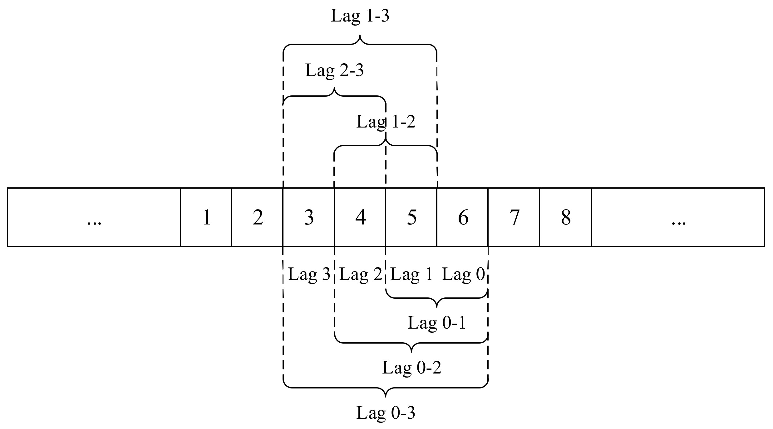
Previous studies showed that the number of lagging months of the vegetation coverage response to explain climatic factors was less than 3 months [39]. Therefore, in this study, the lagging months of the EVI response to explain climatic factors was chosen as 0–3 months, and the time lag of specific months and multiple months was accumulated to determine the response of the vegetation dynamics to the climate. We reconstructed the EVI, and the climate factors associated with time lags of 0–3 months (Figure 2). Here, lags of 0, 1, 2, and 3 months are the remote sensing single month values during the corresponding period and the mean month values during the corresponding time interval.
In this study, regression analysis was conducted to assess the relationship between the time lags of the climate variables and vegetation in each pixel as follows:
E V I x , y = a + i = 0 i = 3 α i x , y T t i + i = 0 i = 3 β i x , y P t i + i = 0 i = 3 γ i x , y H t i + i = 0 i = 3 σ i x , y S t i + ε ,
where T t i , P t i , H t i , and S t i represent the air temperature, precipitation, relative humidity, and sunshine duration for i lag months and time t of the pixel x , y , respectively; ε denotes the residual error; and a is a constant term. In addition, α i , β i , γ i , and σ i are the coefficients for air temperature, precipitation, relative humidity, and sunshine duration, respectively, and E V I represents the standardized EVI monthly average anomaly series.
To eliminate the effect of similar time-varying characteristics and multicollinearity between the climate variables, the Elastic Net (EN) was also applied within each pixel to assign the coefficients of a low influence of climatic factors with parameters of 0 [40,41]. Elastic network regression adds the standard terms to the cost function of linear regression. While the fitting variance is reduced, it has a good coefficient contraction and variable selection effect and eliminates climate factors that only have a weak influence.

2.3.5. The SCS-CN Method

The SCS-CN method calculates runoff using soil classification and rainfall. The general runoff can be expressed as follows:
Q = 0 P I a ( P I a ) 2 P I a + S P > I a
where Q represents the actual direct runoff (mm),   P is the total precipitation (mm), S is the storm rainfall (mm), and I a is initial abstraction (mm). Traditionally, the value of I a is fixed at I a = 0.2 S [42].
The parameter S was calculated according to a dimensionless runoff curve number ( C N ), which varies based on the antecedent moisture condition, land use, and soil types. The parameter S in Equation (7) is related to the value of C N by:
S = 25.4 1000 C N 10
where S is in mm, and C N represents the curve number, which can be found in the TR-55 table.

3. Results

3.1. The Turning Point Detection and the Vegetation Trends

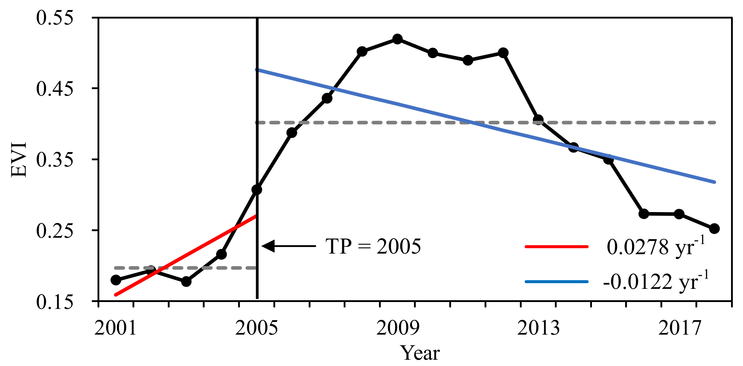
The PELT change point detection method was applied to monitor the offline change points in the annual mean EVI time-series at the regional scale, and the two-part piecewise linear regression model determined the changes in the trends within different periods (Figure 3). The results of the change detection were represented as an inverted V-shaped curve in the EVI time series. The change point occurred in 2005. This indicated that the study area experienced an increase in vegetation coverage from 2001–2005, which was followed by a subsequent decrease from 2006–2018. Based on this turning point, the EVI exhibited a sharp increase at a rate of 0.0278/yr before the turning point (BTP). However, the EVI showed a relative decrease by −0.0122/yr after the turning point (ATP).
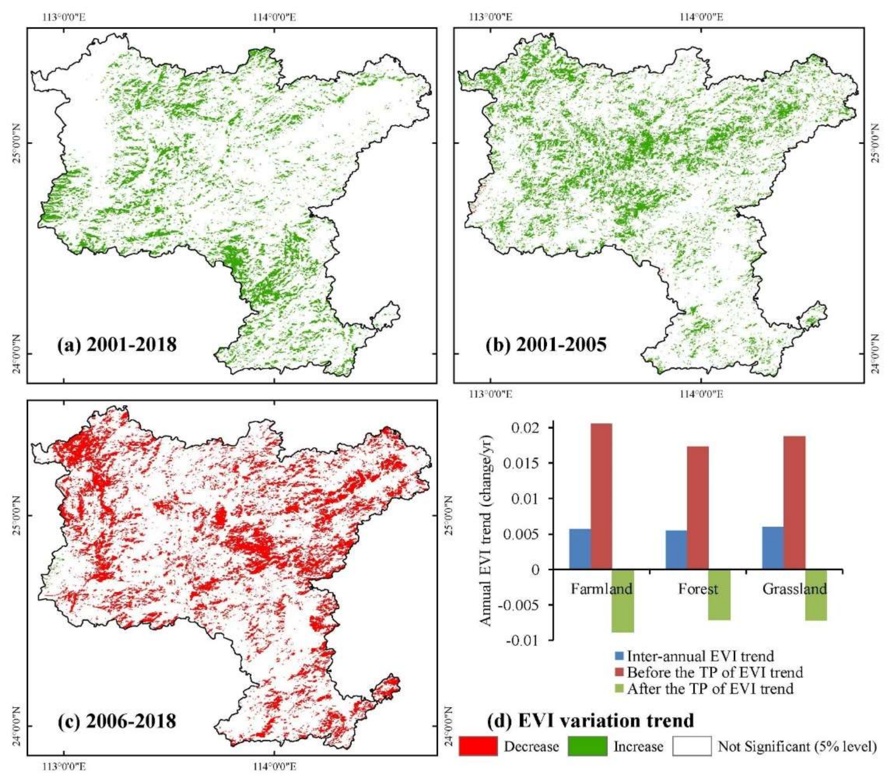
We further investigated the abrupt changes at the pixel scale, and the trends in the annual mean EVI over the last 18 years showed a distinct spatial difference (Figure 4a). While 71% of the study area had no significant trend (stable), a statistically significant upward trend was found for 15% of all pixels, which was mostly concentrated in the southwest region. In contrast, only 1% of the study area showed a significant decrease, which was mostly located in the western region. The trends in the vegetation changes varied greatly for different periods (Figure 4b,c). Before the turning point, 73% of the study area showed no significant trend, and only 25% and 2% were characterized by significant increasing and decreasing trends, respectively. After the breaking point, the vegetation significantly decreased in 33% of the area (distribution throughout the study area). Figure 4d shows the different periods of the vegetation change trends for different land cover types. The inter-annual trend of the mean EVI for different land cover types remains stable. The EVI change trend of farmland showed the quickest increase and decrease before and after the turning point, respectively. Based on the above analysis, farmlands were found to have the most drastic vegetation fluctuations, followed by grasslands and forests.

3.2. Relationships between EVI and Climate Factors

3.2.1. Annual Variations in TEM, PRE, HUM, and SUN

Before analyzing the relationships between EVI and climate factors, we investigated how the TEM, PRE, HUM, and SUN changed from 2001 to 2018. PRE was seen to increase over the 18-year study period (slope = 0.8856 mm/yr) (Table 1), and there were also positive and negative trends in the BTP (slope = 5.0638 mm/yr) and ATP (slope = −0.9869 mm/yr). Both TEM and SUN showed insignificant decreasing trends from 2001 to 2018. In summary, between 2001 and 2018, the fluctuations of the inter-annual climatic factors were concentrated in the PRE, showing a significant increasing trend, while the TEM showed a decreasing trend. These results show that the climate underwent a significant warm–wet change in the study area.

3.2.2. Relationships between EVI and Climate Factors

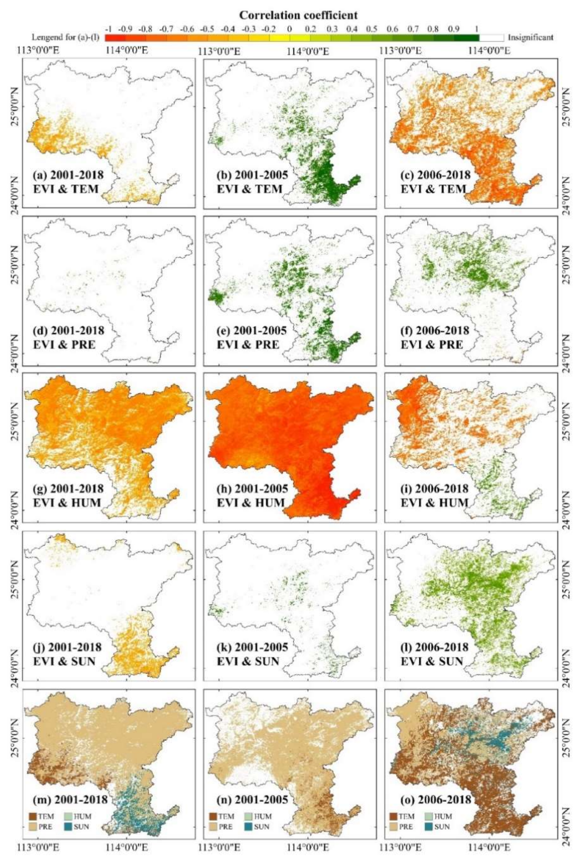
The Pearson correlation coefficients between the annual mean EVI and climate factors (TEM, PRE, HUM, and SUN) were calculated to determine the relationship between the vegetation dynamics and climate variables (Figure 5). PRE was the climate factor with the greatest impact on the EVI variations in 2001–2018 (accounting for 81% of the total study area), followed by TEM (accounting for 10% of the total) and SUN (9%), which mainly impacted the overall EVI trend in the western parts and southern parts of the region, respectively (Figure 5m). PRE (84%) was found to be the climate factor that most strongly influenced the EVI trend in the BTP period. In the ATP period, however, TEM became the main climate factor (57%), having the greatest influence in the southern forest. In BTP, the humidifying trends in the study area first enhanced the vegetation activity. In ATP, such warming trends continued, and the precipitation decrease intensified the water stress loss. In the region where the main influencing climate factors were HUM and TEM, SUN had a minor influence on the vegetation changes.

3.3. Time-Lagged Response of EVI to Climate Factors

3.3.1. Monthly EVI and Climate Factor Variation

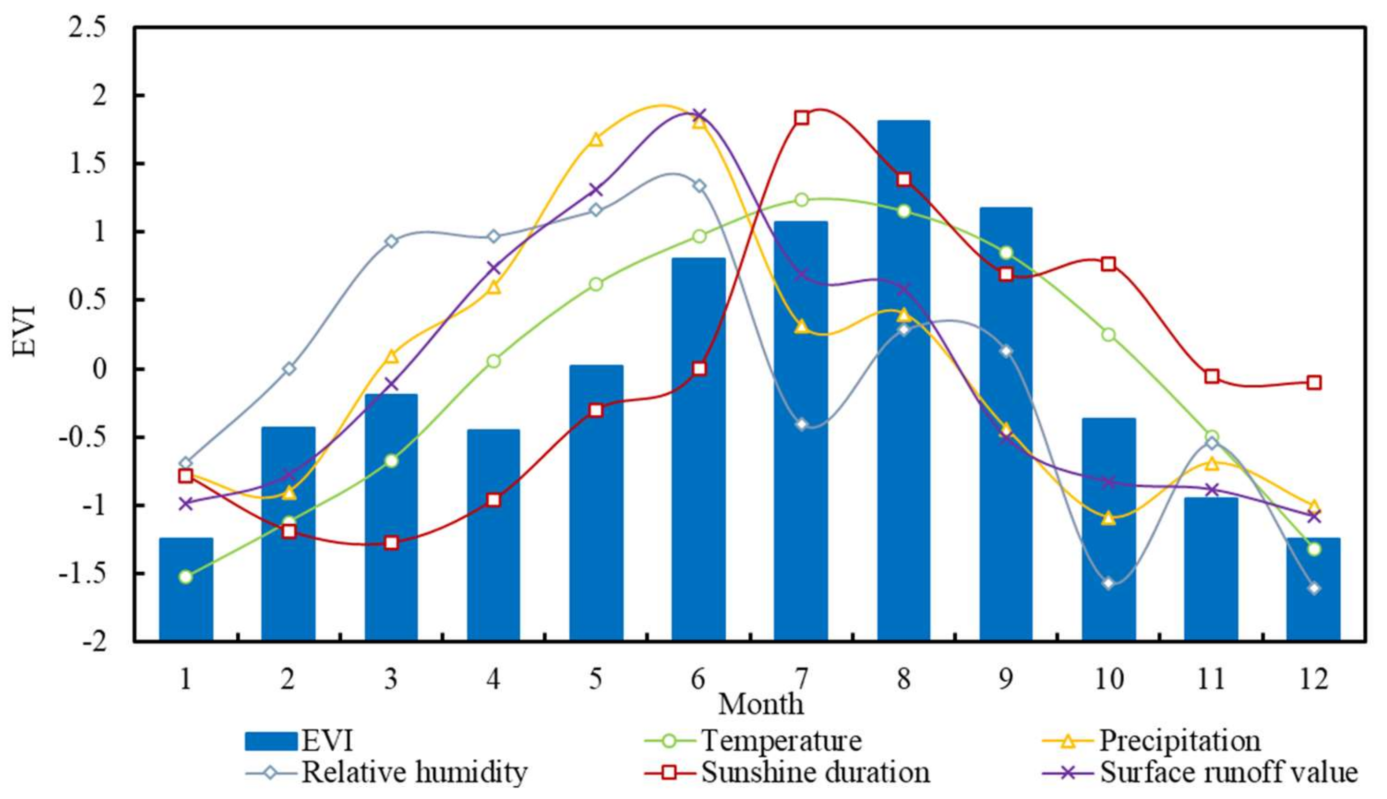
The temporal variations in the inter-annual average EVI and different climate factors from 2001 to 2008 are shown in Figure 6. All trends initially increased and then decreased. Both the EVI and climate factors showed single peaks during the year, with maximum and minimum values in summer and winter, respectively. All factors showed consistency in their changing curves, with upward trends from January to June. However, the sunshine duration, relative humidity, and temperature showed an overall downward trend, with high fluctuations from July to December.
According to the monthly average fluctuations of the EVI and climate factors, the precipitation and relative humidity were found to have increased significantly in May and reached a maximum in June. The maximum values of temperature and sunshine duration occurred in July. The monthly maximum EVI occurred in August, and it lagged behind the climate factors in most years, showing an apparent “time-lag effect” (lagging by 1–3 months in the study area). This phenomenon could be attributed to the high amounts of precipitation in South China [15].

3.3.2. Time-Lagged Effect of Climate Factors

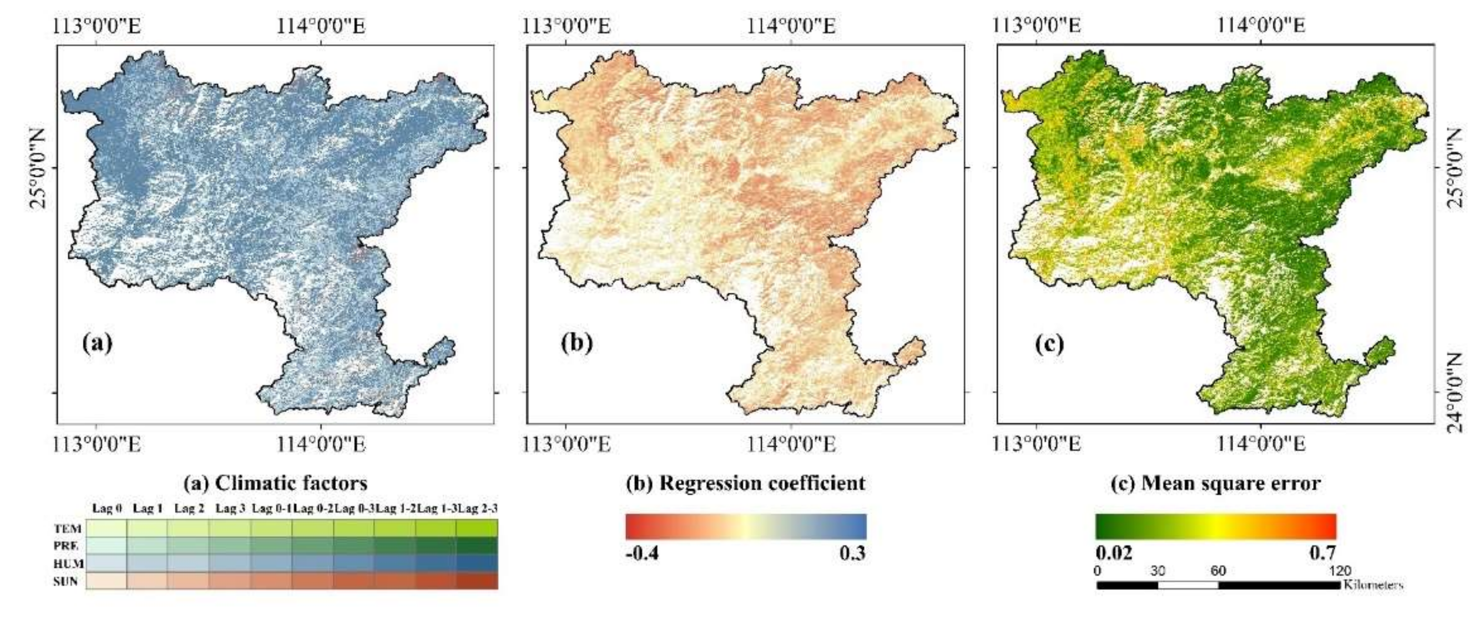
Even though the EVI dynamics result from complex interactions between different climate factors, we expected that various time-lagged climate factors could explain the long time series of the vegetation dynamics. To eliminate the dimensional influence of the different climate factors on the DLM, we normalized each meteorological factor Z-score and then solved the DLM to determine the contribution of each climatic factor to the EVI change. The elastic net solving model eliminates factors that have a low influence, compares the normalization coefficients of the different factors, and identifies the climatic factor with the most substantial influence and its coefficient at the pixel level (Figure 7).
The distribution of the main climate factors affecting changes in the vegetation cover from 2001 to 2018 is shown in Figure 7a. The EVI changes in the study area were mainly influenced by the relative humidity. The highly influenced areas were distributed throughout the region (46.77% of the entire area) and showed a lag period of 0–3 months. Areas that experienced the second-largest influence were mainly distributed in the southwest and southeast (28.16% of the entire area) and showed a lag period of 3 months. Areas dominated by lag periods of 1–3 months and 2–3 months accounted for 1.85% and 0.87% of the total area, respectively, and were scattered in the northwest. Sunshine duration had the second largest influence on the EVI changes, with a lag period of 0–3 months. These areas accounted for 0.85% of the total area and were mainly distributed in regions with a high topographic variability in the north. Areas with lag periods of 3 months accounted for 0.79% of the total area and were mainly located in the south. Areas affected by temperature were scattered across the west and south, accounting for 0.5% of the study area. Precipitation had the lowest areal influence, accounting for 0.13% of the total area. These areas were sporadically distributed across the south.
The DLM was used to calculate the influence of the coefficients of the climate factors on the EVI (Figure 7b). The climate factors had inhibitory effects in most areas (77.98%), with influential coefficients in the range of −0.2 to −0.1. Areas with positive climate impacts were mainly concentrated in the southwest. These areas had influential coefficients in the range of 0.05 to 0.15 and accounted for only 2.63% of the total area. Areas with more robust fits were mainly concentrated in regions with high vegetation EVI values, while lower fits occurred in areas with intense human activity, such as urban areas and regions with a flat topography. The mean square error of the DLM was fitted by the elastic network regression, as shown in Figure 7c. Significant spatial differences in the fitting effect were observed, with the most well-developed fits concentrated in the high EVI areas and the inferior fits concentrated in the urban and hilly areas, where there was intense human activity.
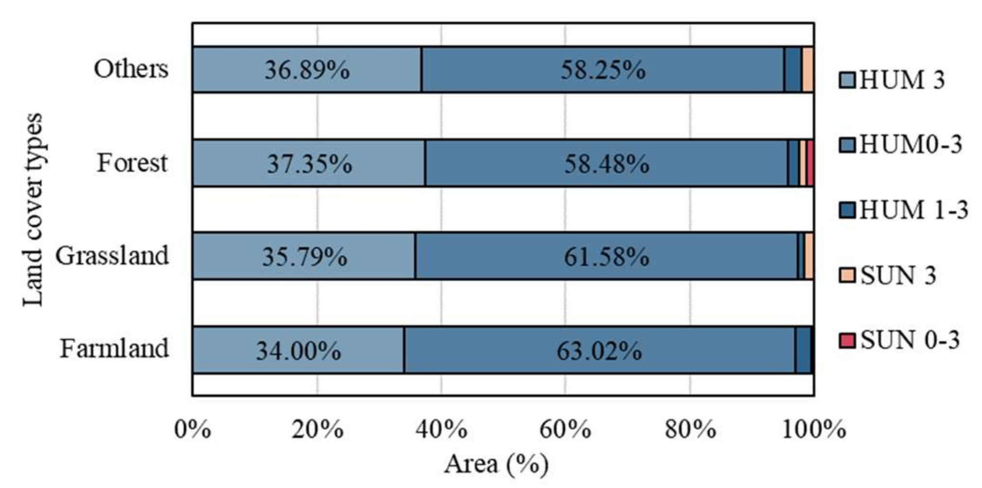
In addition to the climate variables, different time lags occurred in differing land cover categories [24]. Four land cover types were stratified, and Figure 8 shows the time lags for the EVI, relative humidity, and sunshine duration, which cover an area that exceeds 1% of the total area. Raster maps were created to show the time lags of the vegetation response to monthly weather factors for the four land cover types. Farmlands and grasslands were found to have the most considerable lags in relative humidity, and forest land had the shortest lag of three months. The forest time lag had the most significant influence on the sunshine duration, with 1.24% of the area being dominated by a lag of 0–3 months. While there were minimal differences in the time lag difference in response to the sunshine duration between these different land cover types, the total share was mostly the same. Based on the above analysis, farmlands were found to be more sensitive to the cumulative effect of climate factors, followed by grasslands and forests.

3.4. Possible Impact of Vegetation Time Lags on Surface Runoff Depths

Rocky desertification is the most severe problem in karst areas, and a higher surface runoff value can exacerbate the soil erosion effect and exacerbate land degradation. Variations in the EVI, precipitation, and surface runoff value across the year are shown in Figure 6. Almost all surface runoff occurred from March to September, and the runoff increased along with the precipitation in March. There was a rapid decrease in surface runoff when the EVI approached its peak value in August, which indicates that vegetation coverage plays an essential role in controlling soil erosion. When the runoff intensity was at its peak, the EVI values were still relatively low because of the time lag effect. It can be inferred that the increase in vegetation coverage may effectively protect against the occurrence of soil erosion associated with heavy rainfall. A significant decreasing trend (p < 0.001) was evident in the EVI change and surface runoff (Figure 9a), where the change in the EVI was calculated as the difference between the maximum and minimum values of the time series. The accumulated annual surface runoff was obtained using the cumulative runoff during the same year. The average EVI change, and average surface runoff also varied among the different land cover types (Figure 9b). Forests showed a higher average EVI change and a lower average surface runoff. In contrast to the most extended time lag of farmlands, the average EVI change, and average surface runoff are higher. The results show that an increased vegetation cover and shorter time lag can help control the soil erosion in karst areas.

4. Discussion

4.1. Determining the Response of the Vegetation Dynamics to Climate Drivers

This study used a change detection algorithm and piecewise regression models to determine the response of vegetation to climate, and an increasing trend in the EVI index was observed during the study period of 2001–2018. The before and after change points show a forward trend from 2001 to 2018 (Figure 3). These different trends in the spatiotemporal patterns of the vegetation cover indicate that the mountains and valleys provide a significant “corridor barrier” effect in the northeast and in the urban area (Figure 4). There have been no significant temperature changes in South China over the past 20 years; however, there has been an increase in summer precipitation [24], which explains the greening of the vegetation in the karst area [43]. However, extreme climate events in this region have intensified, and the recent drought disaster in Southern China adversely impacted agricultural production [44]. Liu et al. [45] studied the temporal and spatial changes in the vegetation cover within the Qinba Mountains from 2000 to 2014 and identified the turning points in the vegetation trends. Large-scale ecological protection projects have promoted an increase in vegetation cover, and its decline after 2010 may be related to droughts caused by extreme weather. This study also applied the Mann–Kendall test [46] to detect turning points in the EVI time series, and a change point was identified in 2010. Different results were obtained throughout the study area, and a significant jump change point was identified that enabled the EVI time series to be segmented into different stable change segments throughout the study period. Our results (Figure 4) indicate that the EVI time series underwent different annual scale trends, with variations in the land covers, while the inconsistencies in the change magnitude and trend of vegetation greening may indicate the effect of human activities and different change detection algorithms.
Hydrothermal conditions associated with air temperature and precipitation can also significantly impact vegetation growth. The synergistic effect of different climate factors mainly depends on the superposition and cancellation of positive and negative impacts [47]. We compared the BTP and ATP correlations between the different climate factors and the EVI (Figure 5) to determine the effects of each factor on the vegetation change. For the entire study area, a decrease in temperature and a significant increase in the EVI in spring implied the existence of a weakened inhibitory effect on the vegetation EVI in response to the reduced temperature. However, the significant increase in the relative humidity in spring did not significantly inhibit the EVI. The increased relative humidity and vegetation evapotranspiration inhibited vegetation activity, but the increase in the sunshine duration and temperature promoted vegetation growth, resulting in an insignificant increase in the vegetation EVI. An increasing number of studies have found that vegetation growth changes respond to meteorological factors in the southern subtropical monsoon region [48,49]. The negative correlation between the EVI and precipitation was mainly due to local precipitation and temperature exceeding the tree growth threshold. The increase in relative humidity had a significant inhibitory effect on the vegetation EVI. Temperature and precipitation are known to have different impacts on forest phenology, and temperature is the primary driver of spring green-up [50]. The early spring green-up period caused by warming extends the growing season, thereby promoting vegetation EVI. However, the increase in forest cover affects the surface air temperature by altering the energy distribution on the ground surface [51]; therefore, the EVI and air temperature were found to be significantly negatively correlated in the southern hilly areas. The effects of the air temperature, relative humidity, and sunshine duration on the EVI were widely distributed throughout the study area.
The response of the vegetation to the climate lag time varied for different land cover types. We found that farmlands showed the largest lags in response to the relative humidity and sunshine duration, compared to other factors (Figure 8). Kong et al. [16] found that grasslands showed the largest lags for precipitation and temperature change on the Loess Plateau, and Niu et al. [52] found a time lag of 0–96 days in the response of the vegetation to the soil moisture evolution in South China. Precipitation is the only water source for plant growth in many areas. In addition, the water conditions in the valleys are poor, and the EVI is lower than that in the nearby mountains. These factors, coupled with human activities, have resulted in significant reductions in the areas of forests and grasslands [5]. Compared with forests, the ability of other vegetation types to hold soil moisture is limited due to their smaller root systems, and there is a longer time lag in the vegetation green-up [26,53]. Hilly regions in South China are widely affected by mass deforestation in the red soil region and karst region [19]. With respect to ongoing human management, the EVI of farmlands changed drastically during the study period (Figure 9b), and the longer time lag and higher soil erosion in farmlands also relates to the changes in the climate conditions and extreme land cover changes.

4.2. Limitations and Uncertainties

Our study focused exclusively on the effects of climate on vegetation growth, and we did not consider the impacts of human activity or natural disasters. Therefore, future studies could be conducted to consider the impacts of human activities and sudden natural disasters on vegetation EVI. In addition, although the medium-resolution MODIS data used in this study have a high revisit period, it is acknowledged that they lack the ability to accurately describe local vegetation EVI changes. Furthermore, using a linear analysis to determine trends in the response mechanisms of vegetation is challenging, because vegetation change is a nonlinear process [54]; therefore, a nonlinear simulation method that combines terrain, population, and socio-economic factors could also be conducted to effectively determine the impact and response mechanisms involved in vegetation changes.

5. Conclusions

This study used MODIS-EVI and meteorological data from 2001 to 2018 to investigate the change trends and monthly-scale time lags of vegetation cover in relation to the EVI and climate factors within a karst area. Change point detection, correlation analysis, and the DLM method were employed. The influence of vegetation cover on surface runoff was also analyzed. The main findings of this study can be summarized as follows:
At the regional scale, the EVI underwent an overall upward trend during the study period. The EVI first sharply increased before 2005, then showed a relatively weak negative trend change throughout the remainder of the study period. From 2001 to 2018, the EVI change variation in different land cover types (forest, grassland, and farmland) showed a relatively stable trend. Before and after the turning point, however, the EVI trend of farmlands showed the most drastic fluctuation. PRE and TEM were likely the main climate factors. The humidifying trend first enhanced the vegetation activity before 2005, and the continuation of the warming trend likely increased the evaporation of soil water, meaning that there may be further vegetation degradation in the future.
All four climate factors (TEM, PRE, HUM, and SUN) had significant influences on the annual EVI variation. PRE was the climate factor that had the greatest influence on the EVI trends in BTP, accounting for 84%. In ATP, however, TEM was the climate factor that had the greatest influence on the EVI change trend in the southeastern forest areas (57%).
The time lag in response to both the relative humidity and sunshine duration was found to occur mainly three times and 0–3 months later. The time lags between the climatic variables and vegetation change were found to vary by land-cover type. Farmlands exhibited the largest lags, followed by grasslands and forests. These results show that an increase in vegetation cover change, including afforestation and a shorter time lag will help to control the soil erosion in the karst area of North Guangdong.

Author Contributions

Conceptualization, Methodology, Software, Writing: S.W.; methodology: F.F. All authors have read and agreed to the published version of the manuscript.

Funding

This work was supported by the Guangdong Basic and Applied Basic Research Foundation (2021A1515011411).

Institutional Review Board Statement

Not applicable.

Informed Consent Statement

Not applicable.

Data Availability Statement

Not applicable.

Conflicts of Interest

The authors declare no conflict of interest.

References

  1. Potter, C.; Boriah, S.; Steinbach, M.; Kumar, V.; Klooster, S. Terrestrial vegetation dynamics and global climate controls. Clim. Dyn. 2008, 31, 67–78. [Google Scholar] [CrossRef]
  2. Li, Y.; Xie, Z.; Qin, Y.; Zheng, Z. Estimating relations of vegetation, climate change, and human activity: A case study in the 400 mm annual precipitation fluctuation zone, China. Remote Sens. 2019, 11, 1159. [Google Scholar] [CrossRef] [Green Version]
  3. Li, L.; Zhang, Y.; Wu, J.; Li, S.; Zhang, B.; Zu, J.; Zhang, H.; Ding, M.; Paudel, B. Increasing sensitivity of alpine grasslands to climate variability along an elevational gradient on the Qinghai-Tibet Plateau. Sci. Total. Environ. 2019, 678, 21–29. [Google Scholar] [CrossRef] [PubMed]
  4. Tang, J.; Cao, H.; Chen, J. Effects of ecological conservation projects and climate variations on vegetation changes in the source region of the Yangtze River. Acta Geogr. Sin. 2019, 74, 76–86. [Google Scholar]
  5. Gu, Z.; Duan, X.; Shi, Y.; Li, Y.; Pan, X. Spatiotemporal variation in vegetation coverage and its response to climatic factors in the Red River Basin, China. Ecol. Indic. 2018, 93, 54–64. [Google Scholar] [CrossRef]
  6. Li, X.; Li, Y.; Chen, A.; Gao, M.; Slette, I.J.; Piao, S. The impact of the 2009/2010 drought on vegetation growth and terrestrial carbon balance in Southwest China. Agric. For. Meteorol. 2019, 269–270, 239–248. [Google Scholar] [CrossRef]
  7. Li, Z.S.; Liu, G.H.; Fu, B.J.; Zhang, J.L. The potential influence of seasonal climate variables on the net primary production of forests in Eastern China. Environ. Manag. 2011, 48, 1173–1181. [Google Scholar] [CrossRef]
  8. Wang, J.; Wang, K.; Zhang, M.; Zhang, C. Impacts of climate change and human activities on vegetation cover in hilly Southern China. Ecol. Eng. 2015, 81, 451–461. [Google Scholar] [CrossRef]
  9. Li, L.; Zhang, Y.; Liu, L.; Wu, J.; Wang, Z.; Li, S.; Zhang, H.; Zu, J.; Ding, M.; Paudel, B. spatiotemporal patterns of vegetation greenness change and associated climatic and anthropogenic drivers on the Tibetan Plateau during 2000–2015. Remote Sens. 2018, 10, 1525. [Google Scholar] [CrossRef] [Green Version]
  10. Shen, M.; Zhang, G.; Cong, N.; Wang, S.; Kong, W.; Piao, S. Increasing altitudinal gradient of spring vegetation phenology during the last decade on the Qinghai-Tibetan Plateau. Agric. For. Meteorol. 2014, 189, 71–80. [Google Scholar] [CrossRef]
  11. Huete, A.; Liu, H.; Van Leeuwen, W. The use of vegetation indices in forested regions: Issues of linearity and saturation. In Proceedings of the IGARSS 1997 IEEE International Geoscience and Remote Sensing Symposium, Singapore, 3–8 August 1997; Volume 4, pp. 1966–1968. [Google Scholar]
  12. Qu, S.; Wang, L.; Lin, A.; Yu, D.; Yuan, M.; Li, C. Distinguishing the impacts of climate change and anthropogenic factors on vegetation dynamics in the Yangtze River Basin, China. Ecol. Indic. 2020, 108, 105724. [Google Scholar] [CrossRef]
  13. Gurung, R.B.; Breidt, F.J.; Dutin, A.; Ogle, S.M. Predicting Enhanced Vegetation Index (EVI) curves for ecosystem modeling applications. Remote Sens. Environ. 2009, 113, 2186–2193. [Google Scholar] [CrossRef]
  14. Zou, F.; Li, H.; Hu, Q. Responses of vegetation greening and land surface temperature variations to global warming on the Qinghai-Tibetan Plateau, 2001–2016. Ecol. Indic. 2020, 119, 106867. [Google Scholar] [CrossRef]
  15. Xu, G.; Zhang, H.; Chen, B.; Zhang, H.; Innes, J.L.; Wang, G.; Yan, J.; Zheng, Y.; Zhu, Z.; Myneni, R.B. Changes in vegetation growth dynamics and relations with climate over China’s landmass from 1982 to 2011. Remote Sens. 2014, 6, 3263–3283. [Google Scholar] [CrossRef] [Green Version]
  16. Kong, D.; Miao, C.; Wu, J.; Zheng, H.; Wu, S. Time lag of vegetation growth on the Loess Plateau in response to climate factors: Estimation, distribution, and influence. Sci. Total. Environ. 2020, 744, 140726. [Google Scholar] [CrossRef]
  17. Zhao, W.; Qu, X.; Jing, R.; Xiong, K. Spatio-temporal variation of vegetation coverage and its response to climate change in North China plain in the last 33 years. Int. J. Appl. Earth Obs. Geoinf. 2016, 53, 103–117. [Google Scholar] [CrossRef]
  18. Jiang, Z.; Lian, Y.; Qin, X. Rocky desertification in Southwest China: Impacts, causes, and restoration. Earth-Sci. Rev. 2014, 132, 1–12. [Google Scholar] [CrossRef]
  19. Wang, X.; Zhao, X.; Zhang, Z.; Yi, L.; Zuo, L.; Wen, Q.; Liu, F.; Xu, J.; Hu, S.; Liu, B. Assessment of soil erosion change and its relationships with land use/cover change in China from the end of the 1980s to 2010. Catena 2016, 137, 256–268. [Google Scholar] [CrossRef]
  20. Chen, X. Land use change and its impact on water resources in East River Basin, South China. In Watershed Management 2010: Innovations in Watershed Management under Land Use and Climate Change; ASCE: Reston, VA, USA, 2010; pp. 978–989. [Google Scholar]
  21. Wang, X.; Liu, X.; Long, Y.; Liang, W.; Zhou, J.; Zhang, Y. Analysis of Soil retention service function in the North Area of Guangdong based on the InVEST model. In Proceedings of the IOP Conference Series: Earth and Environmental Science; IOP Publishing: Bristol, UK, 2020; Volume 510, p. 032011. [Google Scholar]
  22. Xu, X.; Jiang, H.; Guan, M.; Wang, L.; Huang, Y.; Jiang, Y.; Wang, A. Vegetation responses to extreme climatic indices in coastal China from 1986 to 2015. Sci. Total. Environ. 2020, 744, 140784. [Google Scholar] [CrossRef]
  23. Wu, Y.; Tang, G.; Gu, H.; Liu, Y.; Yang, M.; Sun, L. The variation of vegetation greenness and underlying mechanisms in Guangdong province of China during 2001–2013 based on MODIS data. Sci. Total. Environ. 2019, 653, 536–546. [Google Scholar] [CrossRef]
  24. Yu, L.; Liu, Y.; Liu, T.; Yan, F. Impact of recent vegetation greening on temperature and precipitation over China. Agric. For. Meteorol. 2020, 295, 108197. [Google Scholar] [CrossRef]
  25. Huang, K.; Zhou, T.; Zhao, X. Extreme drought-induced trend changes in MODIS EVI time series in Yunnan, China. In Proceedings of the IOP Conference Series: Earth and Environmental Science; IOP Publishing: Bristol, UK, 2014; Volume 17, p. 12070. [Google Scholar]
  26. Xu, H.J.; Wang, X.P.; Yang, T.B. Trend shifts in satellite-derived vegetation growth in Central Eurasia, 1982–2013. Sci. Total Environ. 2017, 579, 1658–1674. [Google Scholar] [CrossRef]
  27. Wen, Z.; Wu, S.; Chen, J.; Lu, M. NDVI indicated long-term interannual changes in vegetation activities and their responses to climatic and anthropogenic factors in the Three Gorges Reservoir Region, China. Sci. Total. Environ. 2017, 574, 947–959. [Google Scholar] [CrossRef]
  28. Khapalova, E.A.; Jandhyala, V.K.; Fotopoulos, S.B.; Overland, J.E. Assessing change-points in surface air temperature over Alaska. Front. Environ. Sci. 2018, 6, 121. [Google Scholar] [CrossRef]
  29. Rocha, R.V.; de Souza Filho, F.D. Mapping abrupt streamflow shift in an abrupt climate shift through multiple change point methodologies: Brazil case study. Hydrol. Sci. J. 2020, 65, 2783–2796. [Google Scholar] [CrossRef]
  30. Wambui, G.D.; Waititu, G.A.; Wanjoya, A. The power of the pruned exact linear time (PELT) test in multiple changepoint detection. Am. J. Theor. Appl. Stat. 2015, 4, 581. [Google Scholar] [CrossRef] [Green Version]
  31. Wen, Y.; Liu, X.; Pei, F.; Li, X.; Du, G. Non-uniform time-lag effects of terrestrial vegetation responses to asymmetric warming. Agric. For. Meteorol. 2018, 252, 130–143. [Google Scholar] [CrossRef]
  32. Udelhoven, T.; Stellmes, M.; del Barrio, G.; Hill, J. Assessment of rainfall and NDVI anomalies in Spain (1989–1999) using dis-tributed lag models. Int. J. Remote Sens. 2009, 30, 1961–1976. [Google Scholar] [CrossRef]
  33. Ye, Z.-X.; Cheng, W.-M.; Zhao, Z.-Q.; Guo, J.-Y.; Ding, H.; Wang, N. Interannual and seasonal vegetation changes and influencing factors in the extra-high mountainous areas of Southern Tibet. Remote Sens. 2019, 11, 1392. [Google Scholar] [CrossRef] [Green Version]
  34. Merriam, C.F. A comprehensive study of the rainfall on the Susquehanna Valley. Trans. Am. Geophys. Union 1937, 18, 471–476. [Google Scholar] [CrossRef]
  35. Fan, F.; Deng, Y.; Hu, X.; Weng, Q. Estimating composite curve number using an improved SCS-CN method with remotely sensed variables in Guangzhou, China. Remote Sens. 2013, 5, 1425–1438. [Google Scholar] [CrossRef] [Green Version]
  36. Vicente-Serrano, S.M.; Gouveia, C.; Camarero, J.J.; Beguería, S.; Trigo, R.; López-Moreno, J.I.; Azorín-Molina, C.; Pasho, E.; Lorenzo-Lacruz, J.; Revuelto, J.; et al. Response of vegetation to drought time-scales across global land biomes. Proc. Natl. Acad. Sci. USA 2013, 110, 52–57. [Google Scholar] [CrossRef] [PubMed] [Green Version]
  37. Zhang, Q.; Wu, Z.; Yu, H.; Zhu, X.; Shen, Z. Variable urbanization warming effects across metropolitans of China and relevant driving factors. Remote Sens. 2020, 12, 1500. [Google Scholar] [CrossRef]
  38. Li, P.; He, Z.; He, D.; Xue, D.; Wang, Y.; Cao, S. Fractional vegetation coverage response to climatic factors based on grey relational analysis during the 2000–2017 growing season in Sichuan Province, China. Int. J. Remote Sens. 2020, 41, 1170–1190. [Google Scholar] [CrossRef]
  39. Zhao, J.; Huang, S.; Huang, Q.; Wang, H.; Leng, G.; Fang, W. Time-lagged response of vegetation dynamics to climatic and teleconnection factors. Catena 2020, 189, 104474. [Google Scholar] [CrossRef]
  40. Bian, X.; Chen, C.; Xu, Y.; Du, Q. Robust hyperspectral image classification by multi-layer spatial-spectral sparse representations. Remote Sens. 2016, 8, 985. [Google Scholar] [CrossRef] [Green Version]
  41. Lines, J.; Bagnall, A. Time series classification with ensembles of elastic distance measures. Data Min. Knowl. Discov. 2015, 29, 565–592. [Google Scholar] [CrossRef]
  42. Xiao, B.; Wang, Q.-H.; Fan, J.; Han, F.-P.; Dai, Q.-H. Application of the SCS-CN model to runoff estimation in a small watershed with high spatial heterogeneity. Pedosphere 2011, 21, 738–749. [Google Scholar] [CrossRef]
  43. Cai, H.; Yang, X.; Wang, K.; Xiao, L. Is Forest restoration in the Southwest China Karst promoted mainly by climate change or human-induced factors? Remote Sens. 2014, 6, 9895–9910. [Google Scholar] [CrossRef] [Green Version]
  44. Wang, S.; Han, L.; Wang, X.; Zhang, Q.; Lin, J. The affected characteristic of key period’s climate factor on the agricultural disaster loss caused by drought in the South China. Chin. Sci. Bull. 2018, 63, 2378–2392. [Google Scholar] [CrossRef]
  45. Liu, X.; Pan, Y.; Zhu, X.; Li, S. Spatiotemporal variation of vegetation coverage in Qinling-Daba Mountains in relation to envi-ronmental factors. Acta Geogr. Sin. 2015, 70, 705–716. [Google Scholar]
  46. Tong, X.; Wang, K.; Yue, Y.; Brandt, M.; Liu, B.; Zhang, C.; Liao, C.; Fensholt, R. Quantifying the effectiveness of ecological res-toration projects on long-term vegetation dynamics in the Karst regions of Southwest China. Int. J. Appl. Earth Obs. Geoinf. 2017, 54, 105–113. [Google Scholar] [CrossRef] [Green Version]
  47. Lynn, B.H.; Healy, R.; Druyan, L.M. Quantifying the sensitivity of simulated climate change to model configuration. Clim. Chang. 2009, 92, 275–298. [Google Scholar] [CrossRef]
  48. Zhang, X.; Friedl, M.A.; Schaaf, C.B.; Strahler, A.H.; Liu, Z. Monitoring the response of vegetation phenology to precipitation in Africa by coupling MODIS and TRMM instruments. J. Geophys. Res. Space Phys. 2005, 110, 1–14. [Google Scholar] [CrossRef]
  49. Hatfield, J.L.; Prueger, J.H. Temperature extremes: Effect on plant growth and development. Weather Clim. Extrem. 2015, 10, 4–10. [Google Scholar] [CrossRef] [Green Version]
  50. Zhuo, L.; Zhang, Z.; Lei, X.; Li, Q.; Tao, H. Monte Carlo survival analysis on the influencing factors of forest phenology in Northeast China. Acta Geogr. Sin. 2019, 74, 490–503. [Google Scholar]
  51. Ma, D.; Liu, Z.; Lü, S.; Michael, N.; Rong, X.; Cheng, G.; Wang, F. Short-term climatic impacts of afforestation in the East Asian monsoon region. Chin. Sci. Bull. 2013, 58, 2073–2081. [Google Scholar] [CrossRef] [Green Version]
  52. Niu, J.; Chen, J.; Sun, L.; Sivakumar, B. Time-lag effects of vegetation responses to soil moisture evolution: A case study in the Xijiang Basin in South China. Stoch. Environ. Res. Risk Assess. 2017, 32, 2423–2432. [Google Scholar] [CrossRef]
  53. Zhang, J.-T.; Ru, W.; Li, B. Relationships between vegetation and climate on the Loess Plateau in China. Folia Geobot. Phytotaxon. 2006, 41, 151–163. [Google Scholar] [CrossRef]
  54. Leroux, L.; Bégué, A.; Seen, D.L.; Jolivot, A.; Kayitakire, F. Driving forces of recent vegetation changes in the Sahel: Lessons learned from regional and local level analyses. Remote Sens. Environ. 2017, 191, 38–54. [Google Scholar] [CrossRef] [Green Version]
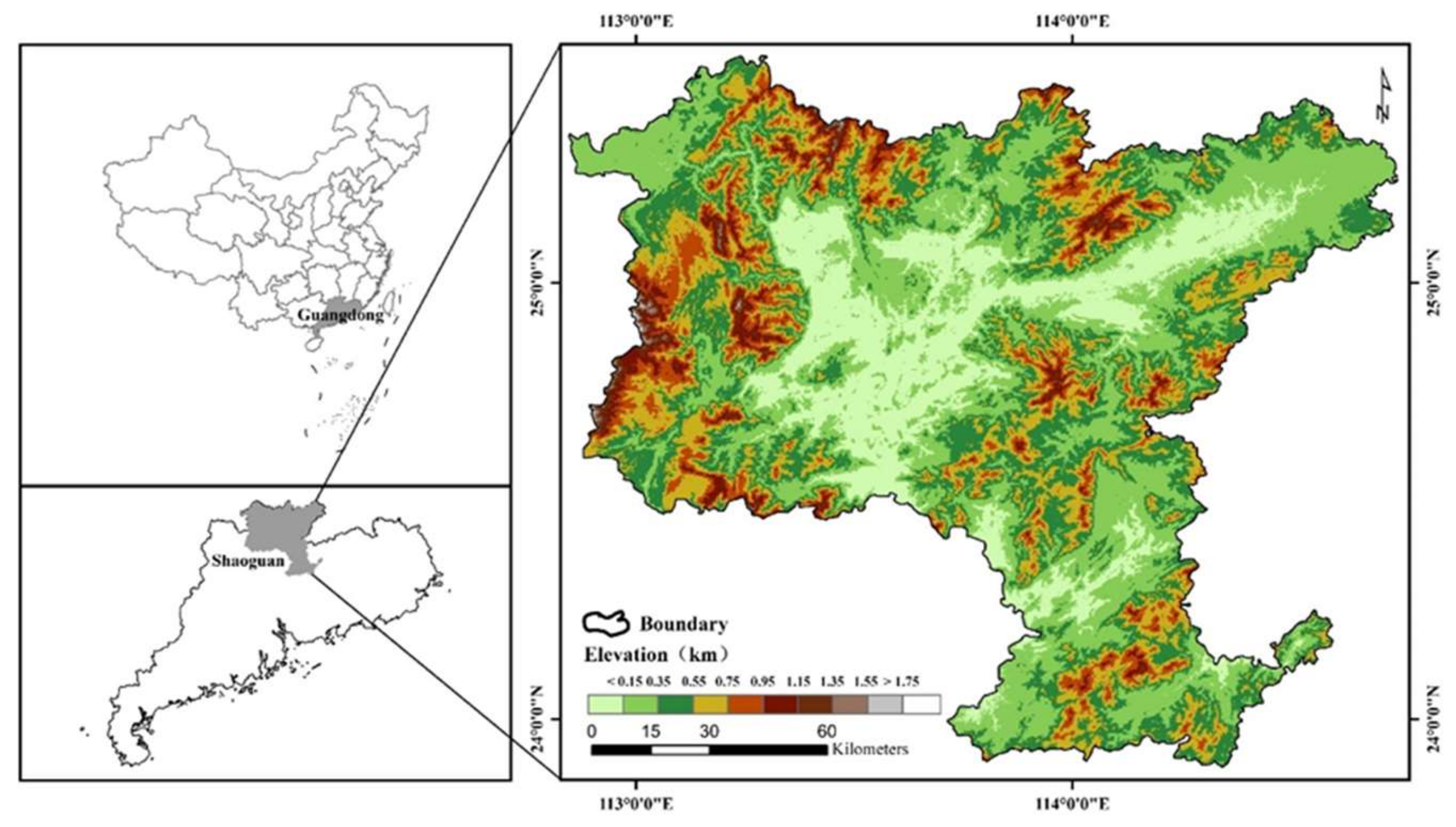
Figure 1. The geographical location of the northern area of Guangdong (China) and digital elevation model.
Remotesensing 13 01873 g001
Figure 2. Sketch illustrating how different periods of lag data were reconstructed using the average calculated over various time windows.
Remotesensing 13 01873 g002
Figure 3. EVI inter-annual variations and linear trends for two periods (2001–2005 and 2006–2018).
Remotesensing 13 01873 g003
Figure 4. (ac) Vegetation trend for different periods: (a) 2001–2018, (b) 2001–2005, and (c) 2006–2018) based on the annual mean EVI. (d) Vegetation trend in different periods for different land cover types.
Remotesensing 13 01873 g004
Figure 5. Spatial distribution of the correlation coefficients between the climate factors and EVI and the main climatic factor in different periods: study period from 2001 to 2018 (a,d,g,j,m), BTP (b,e,h,k,n), and ATP (c,f,i,l,o).
Remotesensing 13 01873 g005
Figure 6. Multi-year monthly mean EVI, temperature, precipitation, relative humidity, sunshine duration, and surface runoff depth during 2001–2018.
Remotesensing 13 01873 g006
Figure 7. Climate-driving forces behind the EVI changes (a), DLM coefficients of the climate factors (b), and the mean square error (c).
Remotesensing 13 01873 g007
Figure 8. Time lags for different land cover types.
Remotesensing 13 01873 g008
Figure 9. (a) Relationship between the change in EVI and annual surface runoff; (b) the EVI change and corresponding average surface runoff for different land cover types.
Remotesensing 13 01873 g009
Table 1. Regression slope, including the overall trend, BTP trend, ATP trend, TEM, PRE, HUM, and SUN at the regional scale for the whole study area.
VariableRegression Slope
Overall TrendBTP TrendATP Trend
TEM−0.00370.0530.0191
PRE0.88565.0638−0.9869
HUM0.1377−1.6385−0.531
SUN−0.69190.2191−0.6632
Publisher’s Note: MDPI stays neutral with regard to jurisdictional claims in published maps and institutional affiliations.