Article

Classifying Forest Type in the National Forest Inventory Context with Airborne Hyperspectral and Lidar Data

1
Remote Sensing and Geospatial Analysis Laboratory, University of Washington, Seattle, WA 98195, USA
2
USDA Forest Service Pacific Northwest Research Station, University of Washington, Seattle, WA 98195, USA
3
Department of Forest Resources, University of Minnesota, Cleveland, MN 55108, USA
4
NASA Goddard Space Flight Center, Greenbelt, MD 20771, USA
*
Author to whom correspondence should be addressed.
Remote Sens. 2021, 13(10), 1863; https://doi.org/10.3390/rs13101863
Submission received: 12 March 2021 / Revised: 16 April 2021 / Accepted: 30 April 2021 / Published: 11 May 2021
(This article belongs to the Section Forest Remote Sensing)

Abstract

:
Forest structure and composition regulate a range of ecosystem services, including biodiversity, water and nutrient cycling, and wood volume for resource extraction. Forest type is an important metric measured in the US Forest Service Forest Inventory and Analysis (FIA) program, the national forest inventory of the USA. Forest type information can be used to quantify carbon and other forest resources within specific domains to support ecological analysis and forest management decisions, such as managing for disease and pests. In this study, we developed a methodology that uses a combination of airborne hyperspectral and lidar data to map FIA-defined forest type between sparsely sampled FIA plot data collected in interior Alaska. To determine the best classification algorithm and remote sensing data for this task, five classification algorithms were tested with six different combinations of raw hyperspectral data, hyperspectral vegetation indices, and lidar-derived canopy and topography metrics. Models were trained using forest type information from 632 FIA subplots collected in interior Alaska. Of the thirty model and input combinations tested, the random forest classification algorithm with hyperspectral vegetation indices and lidar-derived topography and canopy height metrics had the highest accuracy (78% overall accuracy). This study supports random forest as a powerful classifier for natural resource data. It also demonstrates the benefits from combining both structural (lidar) and spectral (imagery) data for forest type classification.

Graphical Abstract

1. Introduction

Forests play an important role in the global carbon cycle, thus forest monitoring is critical to understanding and quantifying forest dynamics and the impact of climate change on forest ecosystems [1,2]. Alaska is the largest state in the USA and the boreal forests within the interior region of the state account for approximately 17% (520,000 km2) of the nation’s forestland. [3]. Interior Alaska is also warming faster than many places on Earth, with a mean annual temperature increase of 2.06 degrees Celsius between 1949–2016 [4,5]. Climate projections indicate continued increases in average annual temperature and precipitation in the coming years, with some models predicting up to five degrees Celsius increase in annual temperature and 50% increase in precipitation by 2080 [6]. These projected changes have potential impacts on livelihoods and resource management. Although much of interior Alaska’s forests are remote and inaccessible, many households within the rural communities of interior Alaska are dependent on the nearby forest resources for heat/energy, building materials, and wildlife habitat [7]. As a result, interior Alaska’s communities are interested in assessing the available supply of forest biomass in Alaska’s forests for use in the production of bioenergy [8]. In addition, understanding biomass and how it is distributed within different forest types in Alaska helps us to quantify and measure changes in boreal forests under climate change [9].
The USDA Forest Service Forest Inventory and Analysis (FIA) program provides vital information for assessing the status of forests in the United States. Prior to 2014, interior Alaska was not included in the FIA program due to the extreme remoteness and inaccessibility of the region. In 2014, a pilot project was established to begin the work of surveying interior Alaska, starting with the Tanana valley region of the state. This area included the Tanana Valley State Forest and Tetlin National Wildlife Refuge, which were sampled at a 1:4 intensity (or one plot per 97.12 km2, or 24,000 acres) on a hexagonal grid [10].
While these new FIA plots were being established for the 2014 Tanana pilot project, high-resolution airborne remote sensing data were acquired by NASA Goddard’s Lidar, Hyperspectral and Thermal (G-LiHT) Airborne Imager to augment the relatively sparse sample of FIA field plots. This new suite of sensors developed by scientists at NASA maps the composition, structure, and function of terrestrial ecosystems with coincident, high (~1 m2) spatial resolution hyperspectral, thermal, and lidar data. [11]. Together, these multi-sensor data provide a novel opportunity to assess forest conditions in the areas covered by the G-LiHT swaths at the scale of individual tree crowns.
One of the standard measures in the FIA plot protocol is the condition class within each plot. Forest type is a primary condition class attribute recorded at each plot and is defined as the species of tree with the dominant stocking of live trees that are not overtopped [12]. In Alaska this essentially records the dominant canopy tree species present at a given plot. If there are no trees present or if the trees do not meet a specific tree canopy cover threshold (10%), then the plot is considered non-forest [13]. These data provide a field reference for the distribution of different species throughout the forests. For species that frequently occur in mixed stands, the dominant species information is a categorical indicator of condition class, not a continuous measure of canopy cover by species. In combination with the G-LiHT data, condition class data for each plot location can be used to classify forest type throughout that Tanana valley of interior Alaska.
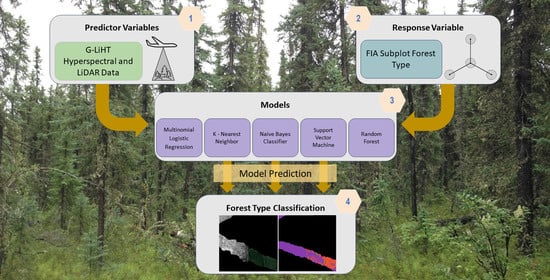
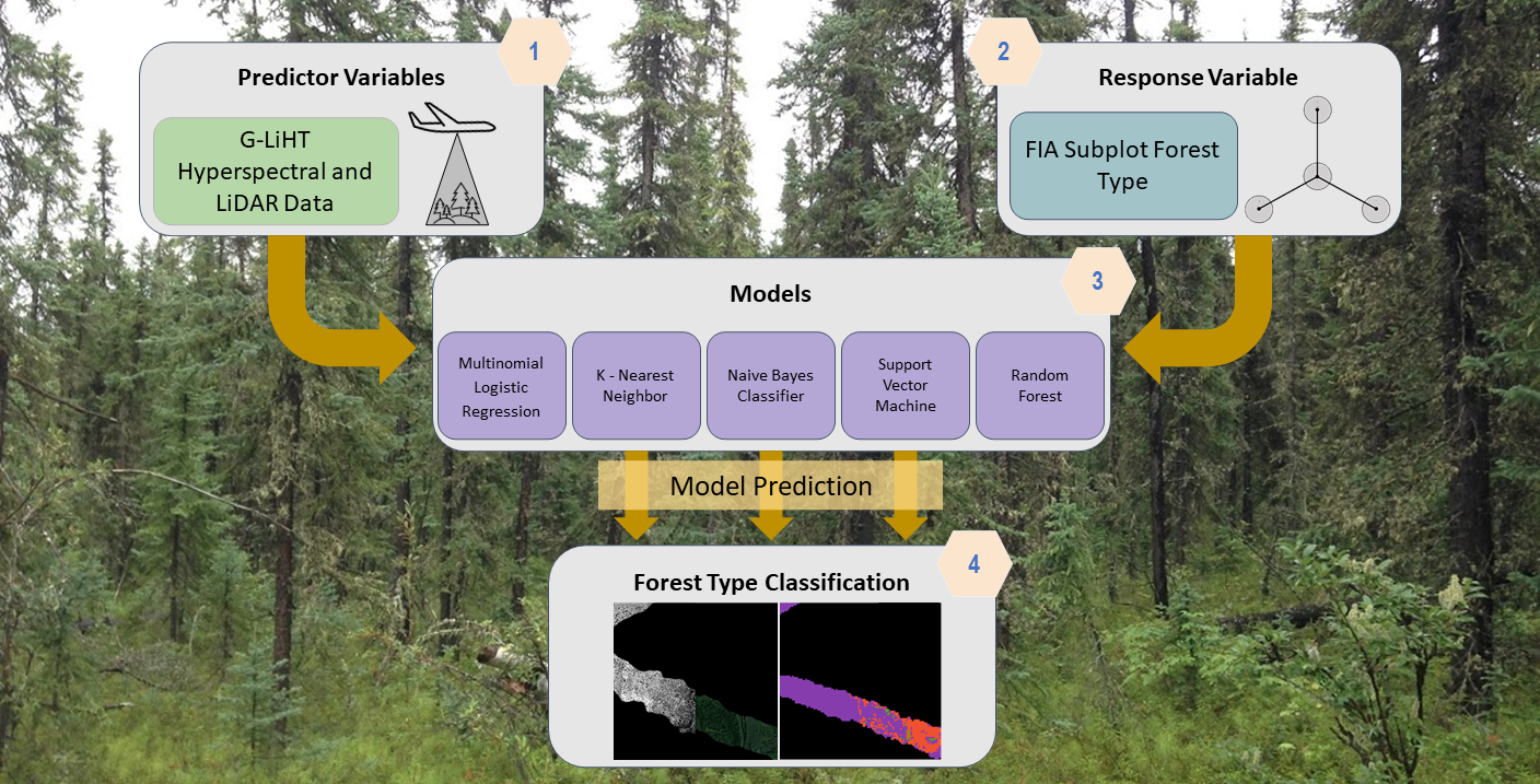
In this study, we developed and applied a methodology for classifying FIA-defined forest type across the Tanana Inventory Unit (TIU) of interior Alaska using the fusion of G-LiHT hyperspectral and lidar data [10,11]. These structural and spectral data from G-LiHT, and the field data from the newly installed FIA plots, provide the information necessary to predict forest type within the TIU. We evaluated different classification algorithms and combinations of hyperspectral and lidar data to identify the model with the highest classification accuracy, and then applied the best model to G-LiHT data across the TIU to compare modeled versus observed forest type information from FIA forest inventory plots. Although interior Alaska has only six main canopy tree species, the combination of small crown sizes, open canopy structure, and mixed stands creates challenges for classifying forest type, even with high-resolution multi-sensor airborne data. Similar studies have used hyperspectral and lidar data to classify tree species with machine learning models [14,15], but none have used the combination to classify forest type, a unique metric in the USDA Forest Service FIA inventory. The potential to accurately classify forest type using airborne remote sensing data is important to support multi-level forest inventories as well as broader assessments in regions where FIA plots were not installed but hyperspectral and lidar data are available.

2. Materials and Methods

2.1. Study Location

This study was conducted within the Tanana Inventory Unit (TIU) located within the Tanana Valley of Interior Alaska (Figure 1).
The TIU covers 136,482 km2 and is dominated by six tree species: black spruce (Picea mariana), white spruce (Picea glauca), tamarack (also referred to as larch, Larix laricina), Alaska paper birch (Betula papyrifera var. neoalaskana), quaking aspen (Populus tremuloides), and balsam poplar (Populus balsamifera). Forests in the TIU often have open canopy structures that promote the establishment and growth of understory and ground cover vegetation, including shrubs such as dwarf birch (Betula spp.) and willow (Salix spp.) [16,17,18,19,20] (Figure 2).

2.2. FIA Field Data

The modern FIA program implements a multi-phase sampling design. The first phase uses ancillary data, such as satellite or aerial imaging, to stratify the land area by cover type. The second phase is the installation and measurement of permanent ground plots, so long as any portion of the plots contain forest land. In the standard FIA inventory implemented in the lower 48 states, the plots are typically established based on a hexagonal tessellation of the landscape, with one ground plot randomly located in each 24.28 km2 (or 6000-acre) hexagon. The plots are laid out such that there is one central subplot, and 3 outer subplots that are each 36.576 m (120 ft) from center-to-center (Figure 3). The 2014 pilot project in the Tanana Valley of Interior Alaska implemented the same plot design within a sparser 97.12 km2 (24,000 acre) regular hexagon grid, due to the cost and accessibility issues associated with these plots [10]. At each subplot, forest type was measured by field crews who determined the dominant species present within each condition and recorded this as forest type. Only one forest type is assigned for each measured condition. This method is standard for all USDA FIA plots collected on public lands throughout the United States and thus could not be modified for the purposes of this study.

2.3. G-LiHT Data

G-LiHT data were acquired in July–August 2014, coincident with the establishment of FIA plots. Airborne data were acquired as a systematic sample of strips, spaced every 9.2 km (Figure 1); additional flight lines were designed to acquire data over other research study sites.
Lidar point clouds were processed to obtain digital terrain models (DTM) from the ground-classified points and canopy height models (CHM) from the highest point in each grid cell, each at 1-m resolution [21]. The DTM was processed to obtain topography metrics using the gdaldem function within the gdalUtils package in R [22], including slope, aspect, topographic roughness index (TRI), topographic position index (TPI), and roughness [23]. The CHM was processed to obtain canopy metrics using the GridSurfaceStats command line utility in FUSION [21]. This resulted in metrics for max height, potential volume, surface area ratio, surface volume, and surface volume ratio. All DTM and CHM metrics were averaged over each circular subplot (7.3 m radius) (Figure 3).
The G-LiHT hyperspectral data were radiometrically calibrated [11] and converted to at-sensor reflectance for 114 bands approximately equally spaced between 418 and 918 nm at 1 m spatial resolution. The hyperspectral data were further processed in R to obtain a variety of hyperspectral vegetation indices, each of which describe a different and unique spectral characteristic of vegetation. In total, 27 metrics were tested to capture the unique characteristics of each forest type. When aggregating the hyperspectral indices, shadow pixels were eliminated by removing pixels that fell into the lower 10% quantile in three indices: Normalized Difference Vegetation Index (NDVI), photochemical reflectance index (PRI), or Red Edge normalized difference vegetation index (RENDVI) [24,25]. These shadow pixels were removed in all vegetation indices before averaging over each circular subplot.
Nine hyperspectral vegetation indices were calculated to estimate vegetation structure (Table 1): Enhanced Vegetation Index (EVI), NDVI Inverse Simple Ratio (ISR NDVI), NDRE Inverse Simple Ratio (ISR NDRE), Normalized Difference in Red Edge (NDRE), Normalized Difference Vegetation Index (NDVI), Simple Ratio (SR), Simple Ratio Red Edge (SR Red Edge), Visible Atmospheric Resistant Index (VARI), and the Green Vegetation Index (VI green).
Six hyperspectral indices were calculated to characterize biochemical pigments in vegetation (Table 2): Pigment Specific Normalized Difference (PSND a and b), Plant Senescence Reflectance Index (PSRI), Pigment Specific Simple Ratio (PSSR a and b), and Structure Insensitive Pigment Index (SIPI).
In addition, six chlorophyll-specific indices were calculated from the 1 m hyperspectral data (Table 3): Chlorophyll Absorption Ratio (CARI), Chlorophyll Index Red-Edge (CI Red Edge), Carter and Miller index (CSM), Carter and Miller red-edge index (CSM Red Edge), Datt Index (Datt), and Modified Chlorophyll Absorption Ratio (MCARI).
Finally, six indices were calculated to evaluate anthocyanin (Table 4) and carotenoid (Table 5) pigment content: Anthocyanin Content Index (ACI), Anthocynanin Reflectance Index (ARI), Modified Anthocynanin Reflectance Index (mARI), Red/Green Ratio Index (RGRI), and two Carotenoid Reflectance Indices (CRI1, CRI2).
Carotenoid Reflectance Index (CRI 1 and 2) describe carotenoid content (Table 5).

2.4. Data Sub-Setting

In total, 632 FIA subplots were covered by the G-LiHT data used in this study. The nested subplot design of FIA plots leads to an issue of pseudo replication. Subplots that lie within the same plot are only 36.576 m (120 ft) from one another, and thus are more likely to be spectrally and texturally similar to each other when compared to plots in different parts of the forest, based on spatial autocorrelation in both forest and topographic characteristics (Figure 3). Consequently, the models are more likely to classify the forest types of these subplots correctly, even if they trained on a different subplot within the same plot. Despite issues of pseudo replication, all subplots were retained in to provide more complete coverage of forest types in the TIU (Table 6), given the small tree sizes and high degree of spatial heterogeneity in vegetation structure, topography, and moisture conditions in the TIU. The dataset itself is small because it was collected using the USDA Forest Service’s FIA methodology that was adapted for use in remote regions of Alaska. This methodology led to a relatively small dataset, making this an ideal case study for evaluating the feasibility of using remote sensing to fill in the gaps where field data could not.
Most studies that focus on the FIA subplots overcome this issue of pseudoreplication by selecting only one subplot per plot and eliminating the remaining plots from the analysis [46,47]. Subsetting to a single subplot per plot in this study would result in an insufficiently representative sample of subplots for both training and validation (Table 6). Thus, all subplots were used in this analysis, but it must be recognized that pseudo replication is present. Until there are enough subplots of each forest type, this issue cannot be addressed further. This is an important tradeoff that comes with using a “real world” dataset rather than experimental study data collected specifically for use with remote sensing. Bootstrap aggregating, or bagging, was tested, but did not improve model performance [48].

2.5. Model Development

We tested five classification algorithms: Random Forest, Support Vector Machine (SVM), K-Nearest Neighbor (KNN), Naive Bayes Classifier (NBC), and Multinomial Logistic Regression. These five algorithms were chosen because they are commonly used in ecological classification studies but have not been simultaneously compared in any other known ecological study. These were also readily available through packages in R, which is a widely used programming language in USDA Forest Service Research and Development. It should be noted that other languages such as MatLab and Python also offer packages to simultaneously compare Machine Learning algorithms.
Random forest is a machine learning algorithm commonly used in ecological studies as it frequently outperforms other algorithms. Random Forest uses an ensemble of decision trees that are split at each node using a random subset of input predictors. This is repeated a set number of times and used to create models for prediction of classes [49,50]. Random forest is unique when compared to other classification algorithms because it estimates the importance of a predictor variable by determining how much the out of bag (OOB) error increases when data for that variable are permuted while others are left unchanged [49]. Of the multiple ways of measuring variable importance, we used mean decrease in accuracy to measure variable importance rather than mean decrease in Gini [51]. Support vector machines use hyperplanes in an n-dimensional space to separate and distinguish distinct classes in a dataset [52,53]. K-Nearest Neighbor classifiers find the k closest training vectors in Euclidean space to the validation set, and determine the class based on a majority vote of the k training vectors [54,55]. A naive Bayes classifier is a probability-based classifier that uses Bayes’ theorem and assumes conditional independence and a Gaussian distribution in the predictor metrics. The model computes the conditional posterior probability of the response and uses that to perform classifications [56,57,58,59]. Multinomial logistic regressions use a logistic regression to predict the probability of different classes given a set of independent predictor variables. In this study, all Multinomial Logistic Regression models were fit using neural networks [60].
These five classification algorithms were tested to determine the best algorithm for classifying forest type from hyperspectral and lidar data. The overall and kappa prediction accuracies for each model were compared among models. Overall prediction accuracy is defined as the rate at which the model correctly predicts a given class, or forest type in this case. It is calculated by taking the sum of the total number of correct predictions divided by the total number of predictions made. Kappa accuracy, or the kappa coefficient of agreement, is a commonly used metric in remote sensing that accounts for the expected error rate. Kappa is calculated by subtracting the expected accuracy (E) from the observed accuracy (O), and dividing that by 1 minus the expected accuracy [61]:
(O − E)/(1 − E)
Though commonly used, the kappa statistic remains controversial in the field of remote sensing, which is why it was used in combination with overall accuracy in this study [62].
When necessary, parameters within the models were tuned to improve accuracy (Table 7). In the case of Random Forest models, 5000 trees were used instead of the default 500 to boost model performance and obtain a more consistent estimation of variable importance between different model runs [51]. The final Random Forest model used 15,000 trees to ensure extremely stable estimates of variable importance [49,51]. When tuning the Support Vector Machine, a variety of tuning parameters were tested (cost values between 10−1 and 102 and gamma values of 0.5, 1, 2). The best parameters were selected from the tuning function and used in the final models with a radial kernel. In the K-Nearest Neighbor models, k values between 0 and 100 were tested to determine the k value that resulted in the highest prediction accuracy. This “best” k value was selected for each model using an optimization script. In the case of the Naive Bayes Classifier and Multinomial Logistic Regression models, all default parameters were used.
We tested six combinations of predictor data with each classification algorithm to investigate the contributions from structural and spectral metrics to overall model accuracy. The predictor inputs can be summarized as four data types: raw hyperspectral bands, hyperspectral vegetation indices, DTM metrics, and CHM metrics. In the first predictor input group, all available data for the subplots were input into the model. This group was not tested in the Multinomial Logistic Regression models as there were too many predictor inputs. In the second predictor group, most of the raw hyperspectral bands (excluding one band each for red, green, blue, near infrared, and red edge) were removed and only the hyperspectral vegetation indices and the DTM and CHM metrics were included. The other four predictor groups consisted of inputs from a single predictor data group: all 114 raw hyperspectral bands, hyperspectral vegetation indices and 5 raw bands (one band each for red, green, blue, near infrared, and red edge; Table 8), DTM metrics, and CHM metrics.
All available subplot data were used in a 3-fold cross validation to ensure that all data were included in both validation and training. K-fold cross validation is a common practice in machine learning [63]. The 3-fold cross validation used in this study held ~33% of the data for validation and ~66% for training, and then was rotated so that different thirds of the data were used in 3 different “folds” for each modeling algorithm tested. Within each of the 3 cross validation sets, the distribution of each forest type remained consistent to ensure that forest type distribution in the validation sets did not impact results when comparing between sets. These models were used to make predictions over the validation data and compared with the known values for each of the 3 models. This ensures that a prediction was made on every data point within the model and reduces the likelihood of overfitting the model by validating and training on the same data. In total, there were 15 separate models (3 models for each of the 5 classification algorithms) which were compared for each response input.

2.6. Model Application

The two best performing models (Random Forest and Multinomial Logistic Regression) were applied over a portion of the TIU to assess model performance over the G-LiHT data swaths. The model predictions were compared with FIA plot designations for forest type where available by overlaying the model prediction raster and the FIA plot locations at a 13 m2 resolution. A 13 m2 resolution was used to compensate for the 1 to 3 m misalignment between the hyperspectral and lidar data. The raster cell that intersected with the plot center was used in comparing the model classification to the FIA plot designation of forest type for that location (Figure 4).

3. Results

3.1. Model Validation

3.1.1. Random Forest

Random forest with hyperspectral vegetation indices, DTM metrics, and CHM metrics as model inputs had the highest accuracy and kappa of all the classification algorithms and model inputs tested, at an overall accuracy of 78% and a kappa of 0.66 (Table 9). The kappa value of 0.66 indicates substantial agreement (0.61 < kappa < 0.8 [64]) between the known and predicted forest types for each subplot. Table 9 shows the combined accuracy of the three validation “folds” tested for the random forest model. Each of these three validation folds consisted of a unique subset of the data, thus by combining the three we were able to get the overall accuracy of the entire dataset.
The kappa value of 0.66 indicates substantial agreement (0.61 < kappa < 0.8 [64]) between the known and predicted forest types for each subplot [64].
When all available data were included in the model (hyperspectral bands and vegetation indices, with DTM and CHM metrics), the results were also promising, with accuracy reaching 75%. In this model, the kappa value, 0.62, also indicated substantial agreement between known and predicted forest type [64]. The other model inputs tested were the individual model inputs: CHM Metrics, Hyperspectral Vegetation Indices, Hyperspectral Bands, and DTM Metrics. These models all resulted in moderate accuracies, with CHM metrics resulting in the highest accuracy at 69% overall and a kappa value of 0.54, indicating just moderate agreement (0.41 < kappa < 0.6 [64]) between known and predicted forest type. The lowest accuracy and kappa were obtained when inputting only hyperspectral bands, with an accuracy of 45% and a kappa of just 0.23. The raw hyperspectral band data was significantly less predictive than the band-derived hyperspectral vegetation indices.

3.1.2. Support Vector Machine

The SVM model had a relatively high accuracy in the “best” model with 74% accuracy and a kappa of 0.60 (Table 10). Once again, the highest accuracy model resulted from the inclusion of three data types, the hyperspectral vegetation indices with DTM and CHM metrics. The second most accurate SVM model was the model with hyperspectral vegetation indices as inputs at 65%, with a kappa value indicating moderate agreement.

3.1.3. K-Nearest Neighbor

The K-Nearest Neighbor (KNN) models had moderate overall accuracy at ~64% overall with almost all model inputs (Table 11). DTM metrics had the lowest accuracy of any KNN model, at just 48% accuracy. The most accurate model included only hyperspectral vegetation indices, but there was not a significant difference in accuracy between this model input and other data combinations (excluding DTM metrics).

3.1.4. Naive Bayes Classifier

Although maximum likelihood models like the Naive Bayes Classifier (NBC) are standard in classification-focused studies, in this case the NBC model performed the worst overall. Of all NBC model inputs tested, the model that included three data types (hyperspectral vegetation indices with DTM and CHM metrics) was the most accurate at 54% overall accuracy and a kappa of 0.38 (Table 12). The worst performing model included only hyperspectral bands and had an overall accuracy of just 20% and a kappa of 0.08.

3.1.5. Multinomial Logistic Regression

The Multinomial Logistic Regression model (MLR) had the third highest overall accuracy at 71% (Table 13). The highest accuracy models were obtained with hyperspectral vegetation indices, with DTM and CHM metrics as model inputs. This is consistent with most other classification algorithms tested in this study. The second most accurate model input was hyperspectral vegetation indices, which was also commonly observed as the second most accurate input in other models.

3.2. Random Forest Model Variable Importance

Random forest with hyperspectral vegetation indices and DTM and CHM metrics as model inputs had the highest overall and kappa accuracy of all the classification algorithms and model inputs tested. Thus, a single model was produced using all subplots. This model was used to assess variable importance. The metric used to assess variable importance was mean decrease in accuracy, a common metric used in Random Forest studies [65,66].
The canopy height model (CHM) values were shown to be the most important predictor, followed by roughness, surface volume ratio, and elevation (DTM). Canopy height is often the single most important lidar variability in forest studies, indicating that different forest types in this region have different canopy heights on average. The roughness and surface volume ratio capture differences in canopy texture between different forest types, and elevation is well known in ecology as a key attribute of site conditions that influences forest type. These predictor variables were followed by the Datt hyperspectral vegetation index [40] and topographic roughness index (TRI). Datt is sensitive to chlorophyll content, an important factor that helps discriminate among forest types. TRI is a topographic index that indicates the texture of the terrain. It is well known that topography is an important predictor of species distribution in plants [67,68]. It should be noted that many of these predictor variables are highly correlated, thus this may not be truly representative of which predictors are most important.

3.3. Forest Type Class Prediction Accuracies

The three most accurate models were the Random Forest, SVM, and MLR models which included hyperspectral vegetation indices and DTM and CHM metrics. For random forest, the confusion matrix shows the model predicted black spruce and paper birch forest types most accurately, and balsam poplar least accurately. The random forest model also frequently confused white spruce with black spruce and paper birch. Black spruce and paper birch are the most common forest types in the TIU, followed by white spruce (Table 14).
Both Random Forest and SVM achieved high accuracies in the two most common classes, paper birch and black spruce, but had lackluster results in the less common classes, tamarack, cottonwood, aspen, and balsam poplar. The MLR model had very different results—it excelled in predicting the least common species and achieved moderate accuracies in the more common species Table 15). None of the three models had high accuracy for cover types with intermediate abundance (white spruce, non-forest). Overall, MLR had more consistently accurate performance when predicting forest type, despite having a slightly lower overall accuracy when compared to the equivalent Random Forest and SVM models.

3.4. Model Application

The models were applied to predict forest type over a portion of the raw G-LiHT collected over the TIU and predictions were compared with FIA plot designations for forest type where available. Random Forest performed well when predicting Non-Forest, Black Spruce, Cottonwood, and Paper Birch. MLR only had high accuracies in predicting paper birch and mid-range accuracies with Non-Forest (Table 16).

4. Discussion

This study aimed to provide an exploratory comparison of techniques for classifying forest type using well known accuracy statistics and widely available FIA data. Previous studies have worked to answer similar questions and achieved promising results. One study compared the accuracies of Support Vector Machines (SVM), K-Nearest Neighbor, and Gaussian maximum likelihood with leave-one-out-covariance algorithms for the classifications of tree species using both hyperspectral and lidar data [14]. They found that the SVM classifier was the most accurate, yielding just over 89% kappa accuracy.
This study also found SVM yielded higher accuracy than the K-Nearest Neighbor classifier, but the Gaussian maximum likelihood (GML) with leave-one-out-covariance algorithm was not tested. Instead, a naive Bayes classifier which is based on GML assumptions was tested and found to perform the worst of any model. This contradicts the findings with the GML model in [14] which found their GML algorithm outperformed the K-Nearest Neighbor algorithm. This difference is likely due to differences in GML and KNN algorithm and model parameters used in each study.
A second study compared the results of classifying seven tree species and a non-forest class in the Southern Alps of Italy using hyperspectral and lidar data with Support Vector Machines and Random Forest [15]. They found that SVM consistently outperformed Random Forest, achieving 95% overall accuracy. This differs from our findings which revealed that Random Forest outperformed SVM models, no matter the model input, achieving 77.53% overall accuracy with the best Random Forest model, and 73.89% with the best SVM model. This is likely due to differences in data pre-processing, especially in the case of hyperspectral data wherein [15] performed a minimum noise fraction transformation to reduce the data dimensionality. Both minimum noise fraction transformations and principal component analyses (PCA) are common data reduction steps when working with hyperspectral data [69]. Neither were performed in this study as it would impact the interpretability of the results and make it challenging to compare across the different algorithms.
A second factor that may have influenced the difference in results between both [14,15] and this study are the model parameters used. In both SVM and KNN models, users must supply parameters to build the models. In this study, optimization scripts were used to test different model parameters and choose those that resulted in the highest accuracy. In the case of the KNN model, 100 different k-values were tested. For the SVM, multiple cost and gamma values were tested. Additionally, this study used a radial kernel for the SVM, while studies [14,15] used different kernels (a Gaussian kernel was used in the 2008 paper [14], and the kernel used in the 2012 paper [15] was not specified). All these differences in parameters used makes for difference in the final results.
Within the training data there could be a significant difference between forest type as defined by the FIA protocol at the scale of a mapped condition (which must meet certain minimum size criteria, >1 acre, etc.) and the tree species present at a given location, or even subplot scale. In the FIA inventory, forest type (on conditions with >10% tree canopy cover) is based on the tree species with the dominant stocking. This means that on any given subplot, the actual forest composition may be much more mixed than is captured by a single forest type class. A subplot with 51% stocking (or tree cover) of white spruce is spectrally very different from a plot that is 100% white spruce, but the methods here treat both examples as the same class. Though this is the method for forest type classification used by the USDA Forest Service throughout the US, it can create challenges when using this data as ground truth for multispectral classification algorithms, and likely contributed to lower accuracies for white spruce and other species that commonly form mixed stands. Future studies may consider using different field validation data and carrying out a hypothesis test to determine if differences in accuracies between models are statistically significant. Additionally, future studies should consider reporting precision and recall, as opposed to overall accuracy, to compare between models [70]. Each of these steps would allow for better reporting of the uncertainty associated with each measure of accuracy and make for better comparison between classification algorithms.
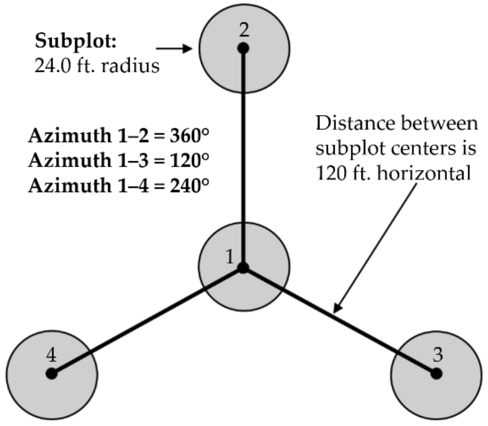
Unlike the potential loss of accuracy due to the spectral mixing within subplots, the nested plot design in this study likely inflated overall accuracy. The FIA protocol is designed such that, for each plot, there are four subplots on which forest type information is collected. There are just 36.576 m (120 ft) between the center subplot and the surrounding three subplots. This leads to an issue of pseudo replication and spatial autocorrelation as the outer three subplots are so close together that they are likely to include similar vegetation. In this study, each subplot was treated as if it was unique and independent of others. This likely led to an inflation in accuracy which cannot be overcome until a more balanced dataset with more equal representation of all forest types within the TIU is available.
Imbalanced datasets are common in ecological studies using natural datasets. While we hope that more data will become available for future research to improve the imbalanced nature of the data in this dataset, we identified multiple ways to overcome the impacts of imbalanced datasets. One common method is to sample the dataset so that there is an equal number of samples in each class that is equal to or less than the size of the smallest class. For example, in this case the smallest forest type class (Tamarack) has four subplots of that class. This methodology would require that for every other forest type class, just four subplots are sampled and used in model training and validation to ensure that the number of samples of each class is the same. This was not feasible in this study because only four samples per class is not enough to train and validate a representative model, so this type of down sampling was not performed.
A second method of overcoming this issue is to oversample the dataset so that each class is sampled with replacement until it reaches a quantity that is typically greater than or equal to the largest class in the dataset. This same methodology can be performed in an ensemble called bootstrap aggregating, or bagging. Bagging is the process by which one samples a dataset D of length n with replacement, to generate a new dataset D1 of length m wherein each class is equally represented [48].
In this case, bagging was implemented in all models to test its impact overall and kappa accuracy. Each class was sampled with replacement until we reached a set equal in length to the largest class within the dataset (280 data points). In most cases, bagging did not improve overall or kappa accuracy. In the cases where accuracy was improved, most models were already performing so poorly that the improved accuracy still did not make the algorithm or model inputs a contender for the best algorithm and inputs. Thus, bagging was not included as a part of this study.
The primary objective of the study was to assess the potential for classifying forest type in the context of a national forest inventory program using high-resolution airborne data. While pseudo replication caused by the nested plot design used in this study, and overfitting of the model in the less common forest types, such as tamarack and poplar, are issues that should be addressed in future studies to provide a full accounting of the classification uncertainty, the results of this study indicate the potential for application of machine learning algorithms to classify forest types in the forest inventory context using a combination of field measurements and high-resolution airborne remote sensing data. As this FIA effort in Alaska continues, leading to more FIA plots and G-LiHT data collected throughout the state, the sample size for every forest type will increase significantly, possibly allowing pseudoreplication to be dealt with by using just one subplot from each plot to represent the entire plot. Alternatively, training and validation datasets could be selected using independent datasets distinct from the FIA field plot sample (at representative sites such as experimental forests, etc.) and then the resulting model could be applied to the FIA field data and G-LiHT data, which would allow for a straightforward assessment of accuracy across the FIA plot sample (although obviously also requiring the collection of an additional, expensive data set).
Future studies could use alternative methods for reducing correlation, and dimensionality, of the input data through PCAs or other techniques. It is also important to note that the variables used in this study are not the only lidar and hyperspectral data-derived metrics that can be used to describe forest composition. There are a multitude of other metrics, from lidar grid metrics to other hyperspectral vegetation indices that have been used in previous studies and may increase model performance [71,72]. Additionally, when aggregating the hyperspectral and lidar metrics over each subplot, using a standard deviation of the metrics instead of or in addition to the average of the metrics may also improve model performance.

5. Conclusions

Overall, the Random Forest classification algorithm resulted in the highest overall and kappa accuracy. There are many factors that make ecological data complex and difficult to model [73,74]. Many studies use Random Forests to overcome these complexities and still yield high prediction accuracies [75,76]. This was likely also the case in this study, resulting in the highest overall accuracy coming from Random Forest.
The MLR model with hyperspectral vegetation indices, DTM metrics, and CHM metrics had the best performance when predicting individual classes, especially rarer classes. This may indicate that the MLR model would be a more suitable model in cases where the objective is to accurately predict rare classes. It also indicates that it may be more suitable to use multiple models when predicting forest type. One could use Random Forest for predicting the more common forest types, and MLR for predicting the less common forest types.
This study also tested a multitude of model inputs and found that including hyperspectral vegetation indices, DTM metrics, and CHM metrics as model inputs yielded the highest overall and kappa accuracy with almost all classification algorithms. Each of these model input groups describe different ecological factors that are essential for distinguishing forest types.
Topography plays an important role in the distribution of vegetation across the landscape, and the topographic variables that can be derived from a DTM can in predicting vegetation distribution [67,77,78]. Unsurprisingly, when these model inputs were tested with all subplots in one Random Forest model, roughness, topographic roughness index, and elevation were found to be extremely important in predicting forest type.
The canopy height model describes the over story structure and can be used to describe species composition when used alongside optical sensors [79,80,81]. In this study, we used both the raw canopy height model and a multitude of CHM-derived metrics to describe the over story. Canopy height was found to be the most important predictor for forest type, with surface volume ratio following close behind.
When it comes to hyperspectral model inputs, including the raw hyperspectral band data with the hyperspectral vegetation indices and CHM and DTM metrics in the Random Forest model decreased accuracy. While it is unclear exactly why this is, we hypothesize that the 114 hyperspectral bands are so highly correlated that they had a negative impact on prediction accuracies. Additionally, transforming the raw hyperspectral data into vegetation indices allows for the data to be relativized, which can boost model performance in many cases.
In summary, this study concluded that:
  • Of all classification algorithms tested, Random Forest resulted in the highest overall and kappa accuracy.
  • A combination of structural and spectral metrics resulted in the highest overall accuracy, including Canopy Height and Digital Terrain model metrics with hyperspectral vegetation indices and five raw hyperspectral bands.

Author Contributions

Conceptualization, L.M.M., H.-E.A. and C.S.; methodology, L.M.M., H.-E.A., C.B. and C.S.; software, C.S., C.B. and H.-E.A.; validation, L.M.M., H.-E.A. and C.S.; formal analysis, C.S.; investigation, C.S., B.D.C. and D.C.M.; resources, L.M.M., H.-E.A., B.D.C. and D.C.M.; data curation, D.C.M. and B.D.C.; writing—original draft preparation, C.S.; writing—review and editing, C.S., L.M.M., H.-E.A., C.B., B.D.C. and D.C.M.; visualization, C.S.; supervision, L.M.M. and H.-E.A.; project administration, C.S., H.-E.A. and L.M.M.; funding acquisition, L.M.M. and H.-E.A. All authors have read and agreed to the published version of the manuscript.

Funding

This study was generously supported by: The USDA Forest Service Pacific Northwest Research Station, The University of Washington Precision Forestry Cooperative, NASA Goddard Space Flight Center, NASA Arctic Boreal Vulnerability Experiment (ABoVE), The University of Washington School of Environmental and Forest Sciences David Briggs Memorial Fellowship.

Institutional Review Board Statement

Not applicable.

Informed Consent Statement

Not applicable.

Data Availability Statement

The FIA data for interior Alaska is publicly available at: https://apps.fs.usda.gov/fia/datamart/datamart_sqlite.html. G-LiHT data products may be viewed and downloaded from the G-LiHT Data Center at https://glihtdata.gsfc.nasa.gov. NASA’s Earth Science Program and promotes the full and open sharing of data with all users, in accordance with NASA’s Data and Information Policy (https://science.nasa.gov/earth-science/earth-science-data/data-information-policy).

Acknowledgments

Thank you to the staff in the University of Washington Precision Forestry Cooperative, USDA Forest Service Pacific Northwest Research Station, University of Washington School of Environmental and Forest Sciences, NASA Goddard Space Flight Center, and NASA Arctic Boreal Vulnerability Experiment (ABoVE). Your advice, assistance, and teaching allowed this research to happen.

Conflicts of Interest

The authors declare no conflict of interest.

References

  1. Andersen, H.-E.; Jacob, S.; Temesgen, H.; Atwood, D.; Winterberger, K. Using multi-level remote sensing and ground data to estimate forest biomass resources in remote regions: A case study in the boreal forests of interior Alaska. Can. J. Remote Sens. 2012, 37, 596–611. [Google Scholar] [CrossRef]
  2. Le Quéré, C.; Raupach, M.R.; Canadell, J.G.; Marland, G.; Bopp, L.; Ciais, P.; Conway, T.J.; Doney, S.C.; Feely, R.A.; Foster, P.; et al. Trends in the sources and sinks of carbon dioxide. Nat. Geosci. 2009, 2, 831–836. [Google Scholar] [CrossRef]
  3. Oswalt, S.N.; Smith, W.B.; Miles, P.D.; Pugh, S.A. Forest Resources of the United States, 2017: A Technical Document Supporting the Forest Service 2020 RPA Assessment; Gen. Tech. Rep. WO-97; U.S. Department of Agriculture, Forest Service, Washington Office: Washington, DC, USA, 2019; Volume 97, p. 223. [CrossRef] [Green Version]
  4. Temperature Changes in Alaska | Alaska Climate Research Center. Available online: http://climate.gi.alaska.edu/ClimTrends/Change/TempChange.html (accessed on 5 May 2019).
  5. McNeeley, S.M.; Shulski, M.D. Anatomy of a closing window: Vulnerability to changing seasonality in Interior Alaska. Glob. Environ. Chang. 2011, 21, 464–473. [Google Scholar] [CrossRef]
  6. Maurer, E.P.; Adam, J.C.; Wood, A.W. Climate model based consensus on the hydrologic impacts of climate change to the Rio Lempa basin of Central America. Hydrol. Earth Syst. Sci. 2009, 13, 183–194. [Google Scholar] [CrossRef] [Green Version]
  7. Wurtz, T.L.; Ott, R.A. Timber Harvest in Interior Alaska; Oxford University Press (OUP): New York, NY, USA, 2006; pp. 302–308. [Google Scholar]
  8. Andersen, H.-E.; Strunk, J.; Temesgen, H. Using Airborne Light Detection and Ranging as a Sampling Tool for Estimating Forest Biomass Resources in the Upper Tanana Valley of Interior Alaska. West. J. Appl. For. 2011, 26, 157–164. [Google Scholar] [CrossRef] [Green Version]
  9. Keith, H.; Mackey, B.G.; Lindenmayer, D.B. Re-evaluation of forest biomass carbon stocks and lessons from the world’s most carbon-dense forests. Proc. Natl. Acad. Sci. USA 2009, 106, 11635–11640. [Google Scholar] [CrossRef] [Green Version]
  10. Andersen, H.-E.; Babcock, C.; Pattison, R.; Cook, B.; Morton, D.; Finley, A. The 2014 Tanana Inventory Pilot: A USFS-NASA Partnership To Leverage Advanced Remote Sensing Technologies for Forest Inventory. In Proceedings of the New Dir. Invent, Techniques and Applications: Forest Inventory and Analysis (FIA) Symposium 2015, Portland, OR, USA, 8–10 December 2015; pp. 40–41. [Google Scholar]
  11. Cook, B.D.; Corp, L.A.; Nelson, R.F.; Middleton, E.M.; Morton, D.C.; McCorkel, J.T.; Masek, J.G.; Ranson, K.J.; Ly, V.; Montesano, P.M. NASA Goddard’s LiDAR, Hyperspectral and Thermal (G-LiHT) Airborne Imager. Remote Sens. 2013, 5, 4045–4066. [Google Scholar] [CrossRef] [Green Version]
  12. Bechtold, W.A.; Patterson, P.L. The Enhanced Forest Inventory and Analysis Program-National Sampling Design and Estimation Procedures; Department of Agriculture, Forest Service, Southern Research Station: Asheville, NC, USA, 2005. [Google Scholar]
  13. Field Instructions for the Annual Inventory of Alaska 2018 Supplement for: Interior Alaska; Department of Agriculture, Forest Service, Pacific Northwest Research Station: Portland, OR, USA, 2018.
  14. Dalponte, M.; Bruzzone, L.; Gianelle, D. Fusion of Hyperspectral and LIDAR Remote Sensing Data for Classification of Complex Forest Areas. IEEE Trans. Geosci. Remote Sens. 2008, 46, 1416–1427. [Google Scholar] [CrossRef] [Green Version]
  15. Dalponte, M.; Bruzzone, L.; Gianelle, D. Tree species classification in the Southern Alps based on the fusion of very high geometrical resolution multispectral/hyperspectral images and LiDAR data. Remote Sens. Environ. 2012, 123, 258–270. [Google Scholar] [CrossRef]
  16. Burns, R.M.; Honkala, B.H. Silvics of North America: Volume 1. Conifers; For. Serv. Agric. Handb. 654; United States Dep. Agric. (USDA): Washington, DC, USA, 1990.
  17. Burns, R.M.; Honkala, B.H. Silvics of North America: Volume 2. Hardwoods; For. Serv. Agric. Handb. 654; United States Dep. Agric. (USDA): Washington, DC, USA, 1990.
  18. Viereck, L.A.; Dyrness, C.T.; Batten, A.R.; Wenzlick, K.J. The Alaska Vegetation Classification; Department of Agriculture, Forest Service, Pacific Northwest Research Station: Portland, OR, USA, 1992; p. 286. [Google Scholar]
  19. Roland, C.A.; Schmidt, J.H.; Nicklen, E.F. Landscape-scale patterns in tree occupancy and abundance in subarctic Alaska. Ecol. Monogr. 2013, 83, 19–48. [Google Scholar] [CrossRef]
  20. Ene, L.T.; Gobakken, T.; Andersen, H.-E.; Næsset, E.; Cook, B.D.; Morton, D.C.; Babcock, C.; Nelson, R. Large-area hybrid estimation of aboveground biomass in interior Alaska using airborne laser scanning data. Remote Sens. Environ. 2018, 204, 741–755. [Google Scholar] [CrossRef]
  21. Mcgaughey, R.J. FUSION/LDV: Software for LIDAR Data Analysis and Visualization; Department of Agriculture, Forest Service, Pacific Northwest Research Station: Seattle, WA, USA, 2018. [Google Scholar]
  22. Greenberg, J.A.; Mattiuzzi, M. gdalUtils: Wrappers for the Geospatial Data Abstraction Library (GDAL) Utilities. CRAN. 2018. Available online: https://CRAN.R-project.org/package=gdalUtils (accessed on 6 May 2021).
  23. Wilson, M.F.J.; O’Connell, B.; Brown, C.; Guinan, J.C.; Grehan, A.J. Multiscale Terrain Analysis of Multibeam Bathymetry Data for Habitat Mapping on the Continental Slope. Mar. Geodesy 2007, 30, 3–35. [Google Scholar] [CrossRef] [Green Version]
  24. Azevedo, S.C.; Silva, E.A.; Pedrosa, M.M. Shadow detection improvement using spectral indices and morphological operators in high resolution images from urban areas. ISPRS Int. Arch. Photogramm. Remote Sens. Spat. Inf. Sci. 2015, XL-7/W3, 587–592. [Google Scholar] [CrossRef] [Green Version]
  25. Liu, X.; Hou, Z.; Shi, Z.; Bo, Y.; Cheng, J. A shadow identification method using vegetation indices derived from hyperspectral data. Int. J. Remote Sens. 2017, 38, 5357–5373. [Google Scholar] [CrossRef]
  26. Huete, A.R.; Liu, H.Q.; Batchily, K.; van Leeuwen, W. A comparison of vegetation indices over a global set of TM images for EOS-MODIS. Remote Sens. Environ. 1997, 59, 440–451. [Google Scholar] [CrossRef]
  27. Gong, P.; Pu, R.; Biging, G.; Larrieu, M. Estimation of forest leaf area index using vegetation indices derived from hyperion hyperspectral data. IEEE Trans. Geosci. Remote Sens. 2003, 41, 1355–1362. [Google Scholar] [CrossRef] [Green Version]
  28. Torino, M.S.; Ortiz, B.V.; Fulton, J.P.; Balkcom, K. Evaluation of Differences In Corn Biomass and Nitrogen Uptake at Various Growth Stages Using Spectral Vegetation Indices. ispag. org. Available online: https://www.ispag.org/abstract_papers/papers/abstract_1251.pdf (accessed on 4 May 2021).
  29. Gitelson, A.; Merzlyak, M.N. Spectral Reflectance Changes Associated with Autumn Senescence of Aesculus hippocastanum L. and Acer platanoides L. Leaves. Spectral Features and Relation to Chlorophyll Estimation. J. Plant Physiol. 1994, 143, 286–292. [Google Scholar] [CrossRef]
  30. Rouse, J.W.J.; Haas, R.H.; Schell, J.A.; Deering, D.W. Monitoring Vegetation Systems in the Great Plains with ERTS; Remote Sensing Center, Texas A&M University: College Station, TX, USA, 1974. [Google Scholar]
  31. Jordan, C.F. Derivation of Leaf-Area Index from Quality of Light on the Forest Floor. Ecology 1969, 50, 663–666. [Google Scholar] [CrossRef]
  32. Gitelson, A.A.; Kaufman, Y.J.; Stark, R.; Rundquist, D. Novel algorithms for remote estimation of vegetation fraction. Remote Sens. Environ. 2002, 80, 76–87. [Google Scholar] [CrossRef] [Green Version]
  33. Blackburn, G.A. Quantifying Chlorophylls and Caroteniods at Leaf and Canopy Scales: An Evaluation of Some Hyperspectral Approaches. Remote Sens. Environ. 1998, 66, 273–285. [Google Scholar] [CrossRef]
  34. Merzlyak, M.N.; Gitelson, A.A.; Chivkunova, O.B.; Rakitin, V.Y. Non-destructive optical detection of pigment changes during leaf senescence and fruit ripening. Physiol. Plant. 1999, 106, 135–141. [Google Scholar] [CrossRef] [Green Version]
  35. Blackburn, G.A. Spectral indices for estimating photosynthetic pigment concentrations: A test using senescent tree leaves. Int. J. Remote Sens. 1998, 19, 657–675. [Google Scholar] [CrossRef]
  36. Firelella, I.; Baret, F.; Peñuelas, J. Semi-empirical indices to asses carotenoids/clorophila a ratio from leaf spectral reflectance. Photosynth 1995, 31, 10. [Google Scholar]
  37. Kim, M.S.; Daughtry, C.S.T.; Chappelle, E.W.; Mcmurtrey, J.E.; Walthall, C.L. The use of high spectral resolution bands for estimating absorbed photosynthetically active radiation (A par). In Proceedings of the 6th Symp. on Physical Measurements and Signatures in Remote Sensing, Val D’Isere, France, 17–21 January 1994; pp. 299–306. [Google Scholar]
  38. Gitelson, A.A.; Keydan, G.P.; Merzlyak, M.N. Three-band model for noninvasive estimation of chlorophyll, carotenoids, and anthocyanin contents in higher plant leaves. Geophys. Res. Lett. 2006, 33, L11402. [Google Scholar] [CrossRef] [Green Version]
  39. Carter, G.A.; Miller, R.L. Early detection of plant stress by digital imaging within narrow stress-sensitive wavebands. Remote Sens. Environ. 1994, 50, 295–302. [Google Scholar] [CrossRef]
  40. Datt, B. Visible/near infrared reflectance and chlorophyll content in Eucalyptus leaves. Int. J. Remote Sens. 1999, 20, 2741–2759. [Google Scholar] [CrossRef]
  41. Daughtry, C. Estimating Corn Leaf Chlorophyll Concentration from Leaf and Canopy Reflectance. Remote Sens. Environ. 2000, 74, 229–239. [Google Scholar] [CrossRef]
  42. Berg, A.K.V.D.; Perkins, T.D. Nondestructive Estimation of Anthocyanin Content in Autumn Sugar Maple Leaves. HortScience 2005, 40, 685–686. [Google Scholar] [CrossRef] [Green Version]
  43. Gitelson, A.A.; Merzlyak, M.N.; Chivkunova, O.B. Optical Properties and Nondestructive Estimation of Anthocyanin Content in Plant Leaves. Photochem. Photobiol. 2007, 74, 38–45. [Google Scholar] [CrossRef]
  44. Gamon, J.A.; Surfus, J.S. Assessing leaf pigment content and activity with a reflectometer. New Phytol. 1999, 143, 105–117. [Google Scholar] [CrossRef]
  45. Gitelson, A.A.; Zur, Y.; Chivkunova, O.B.; Merzlyak, M.N. Assessing Carotenoid Content in Plant Leaves with Reflectance Spectroscopy. Photochem. Photobiol. 2002, 75, 272–281. [Google Scholar] [CrossRef]
  46. Hurlbert, S.H. Pseudoreplication and the Design of Ecological Field Experiments. Ecol. Monogr. 1984, 54, 187–211. [Google Scholar] [CrossRef] [Green Version]
  47. Weishampel, P.; Kolka, R.; King, J.Y. Carbon pools and productivity in a 1-km2 heterogeneous forest and peatland mosaic in Minnesota, USA. For. Ecol. Manag. 2009, 257, 747–754. [Google Scholar] [CrossRef]
  48. Breiman, L. Bagging Predictors. Mach. Learn. 1996, 24, 123–140. [Google Scholar] [CrossRef] [Green Version]
  49. Liaw, A.; Wiener, M. Classification and Regression by randomForest; R Project: Vienna, Austria, 2002; Volume 2/3. [Google Scholar]
  50. Breiman, L. Random Forests. Mach. Learn. 2001, 45, 5–32. [Google Scholar] [CrossRef] [Green Version]
  51. Breiman, L. Manual on Setting Up, Using, and Understanding Random Forests V3.1; UC Berkeley Statistics Department: Berkeley, CA, USA, 2002. [Google Scholar]
  52. Chang, C.-C.; Lin, C.-J. LIBSVM: A Library for Support Vector Machines; Taiwan University Department of Computer Science and Information Engineering: Taipei, Taiwan, 2001; Available online: https://www.csie.ntu.edu.tw/~cjlin/libsvm/ (accessed on 4 May 2021).
  53. Cheriet, M.; Adankon, M.M. Support Vector Machine. In Encyclopedia of Biometrics; Springer: Boston, MA, USA, 2009; pp. 1303–1308. [Google Scholar]
  54. Ripley, B.D. Pattern Recognition and Neural Networks; Cambridge University Press: Cambridge, UK, 2007; ISBN 0521717701. [Google Scholar]
  55. Peterson, L.E. K-nearest neighbor. Scholarpedia 2009, 4, 1883. [Google Scholar] [CrossRef]
  56. Hand, D.J.; Yu, K. Idiot’s Bayes: Not so Stupid after All? Int. Stat. Rev. 2001, 69, 385. [Google Scholar] [CrossRef]
  57. Zhang, H. The Optimality of Naïve Bayes. In Proceedings of the Seventeenth International Florida Artificial Intelligence Research Society Conference, Miami Beach, FL, USA, 12–14 May 2004. [Google Scholar]
  58. Murphy, K.P. Naive Bayes Classifiers; University of British Columbia: Vancouver, BC, Canada, 2006. [Google Scholar]
  59. Leung, K.M. Naive Bayesian Classifier; Polytechnic University Department of Computer Science/Finance and Risk Engineering: Hong Kong, China, 2007. [Google Scholar]
  60. Kwak, C.; Clayton-Matthews, A. Multinomial Logistic Regression. Nurs. Res. 2002, 51, 404–410. [Google Scholar] [CrossRef] [PubMed]
  61. Kuhn, M. Building Predictive Models inRUsing thecaretPackage. J. Stat. Softw. 2008, 28, 1–26. [Google Scholar] [CrossRef] [Green Version]
  62. Pontius, R.G., Jr.; Millones, M. Death to Kappa: Birth of quantity disagreement and allocation disagreement for accuracy assessment. Int. J. Remote Sens. 2011, 32, 4407–4429. [Google Scholar] [CrossRef]
  63. Jung, Y. Multiple predictingK-fold cross-validation for model selection. J. Nonparametr. Stat. 2018, 30, 197–215. [Google Scholar] [CrossRef]
  64. Landis, J.R.; Koch, G.G. The Measurement of Observer Agreement for Categorical Data. Biometrics 1977, 33, 159–174. [Google Scholar] [CrossRef] [PubMed] [Green Version]
  65. Schroeder, T.A.; Schleeweis, K.G.; Moisen, G.G.; Toney, C.; Cohen, W.B.; Freeman, E.A.; Yang, Z.; Huang, C. Testing a Landsat-based approach for mapping disturbance causality in U.S. forests. Remote Sens. Environ. 2017, 195, 230–243. [Google Scholar] [CrossRef] [Green Version]
  66. Derwin, J.M.; Thomas, V.A.; Wynne, R.H.; Coulston, J.W.; Liknes, G.C.; Bender, S.; Blinn, C.E.; Brooks, E.B.; Ruefenacht, B.; Benton, R.; et al. Estimating tree canopy cover using harmonic regression coefficients derived from multitemporal Landsat data. Int. J. Appl. Earth Obs. Geoinf. 2020, 86, 101985. [Google Scholar] [CrossRef]
  67. Florinsky, I.V.; Kuryakova, G.A. Influence of topography on some vegetation cover properties. Catena 1996, 27, 123–141. [Google Scholar] [CrossRef]
  68. Gracia, M.; Montané, F.; Piqué, J.; Retana, J. Overstory structure and topographic gradients determining diversity and abundance of understory shrub species in temperate forests in central Pyrenees (NE Spain). For. Ecol. Manag. 2007, 242, 391–397. [Google Scholar] [CrossRef]
  69. Zhang, Z.; Kazakova, A.; Moskal, L.M.; Styers, D.M. Object-Based Tree Species Classification in Urban Ecosystems Using LiDAR and Hyperspectral Data. Forests 2016, 7, 122. [Google Scholar] [CrossRef] [Green Version]
  70. Davis, J.; Goadrich, M. The relationship between Precision-Recall and ROC curves. In Proceedings of the 23rd International Conference on Machine Learning, Pittsburgh, PA, USA, 25–29 June 2006; pp. 233–240. [Google Scholar]
  71. Cao, Q.; Miao, Y.; Wang, H.; Huang, S.; Cheng, S.; Khosla, R.; Jiang, R. Non-destructive estimation of rice plant nitrogen status with Crop Circle multispectral active canopy sensor. Field Crop. Res. 2013, 154, 133–144. [Google Scholar] [CrossRef]
  72. Hunt, E.R.; Doraiswamy, P.C.; McMurtrey, J.E.; Daughtry, C.S.; Perry, E.M.; Akhmedov, B. A visible band index for remote sensing leaf chlorophyll content at the canopy scale. Int. J. Appl. Earth Obs. Geoinf. 2013, 21, 103–112. [Google Scholar] [CrossRef] [Green Version]
  73. Breiman, L. Statistical Modeling: The Two Cultures (with comments and a rejoinder by the author). Stat. Sci. 2001, 16, 199–231. [Google Scholar] [CrossRef]
  74. Olden, J.D.; Lawler, J.J.; Poff, N.L. Machine Learning Methods Without Tears: A Primer for Ecologists. Q. Rev. Biol. 2008, 83, 171–193. [Google Scholar] [CrossRef] [Green Version]
  75. Rodriguez-Galiano, V.; Ghimire, B.; Rogan, J.; Chica-Olmo, M.; Rigol-Sanchez, J. An assessment of the effectiveness of a random forest classifier for land-cover classification. ISPRS J. Photogramm. Remote Sens. 2012, 67, 93–104. [Google Scholar] [CrossRef]
  76. Cutler, D.R.; Edwards, T.C., Jr.; Beard, K.H.; Cutler, A.; Hess, K.T.; Gibson, J.; Lawler, J.J. Random forests for classification in ecology. Source Ecol. UTC Ecol. 2007, 88, 2783–2792. [Google Scholar] [CrossRef] [PubMed]
  77. Brown, D.G. Predicting vegetation types at treeline using topography and biophysical disturbance variables. J. Veg. Sci. 1994, 5, 641–656. [Google Scholar] [CrossRef] [Green Version]
  78. Wang, B.; Zhang, G.; Duan, J. Relationship between topography and the distribution of understory vegetation in a Pinus massoniana forest in Southern China. Int. Soil Water Conserv. Res. 2015, 3, 291–304. [Google Scholar] [CrossRef] [Green Version]
  79. Dubayah, R.O.; Drake, J.B. Lidar Remote Sensing for Forestry. J. For. 2000, 98, 44–46. [Google Scholar] [CrossRef]
  80. Dubayah, R.; Blair, J.B.; Bufton, J.L.; Clark, D.; Jaja, J.; Knox, R.; Luthcke, S.B.; Prince, S.; Weishampel, J.F. The vegetation canopy lidar mission. L. Satell. Inf. Next Decad. II Sources Appl. 1997, 100–112. [Google Scholar]
  81. Hudak, A.T.; Bright, B.C.; Pokswinski, S.M.; Loudermilk, E.L.; O’Brien, J.J.; Hornsby, B.S.; Klauberg, C.; Silva, C.A. Mapping Forest Structure and Composition from Low-Density LiDAR for Informed Forest, Fuel, and Fire Management at Eglin Air Force Base, Florida, USA. Can. J. Remote Sens. 2016, 42, 411–427. [Google Scholar] [CrossRef]
Figure 1. Tanana Inventory Unit Boundary (orange) and 2014 G-LiHT Flight lines (black) with Google Streets as basemap.
Remotesensing 13 01863 g001
Figure 2. Example of black spruce forest structure in the Tanana Inventory Unit with significant understory component in the form of small shrubs, lichen, and mosses.
Remotesensing 13 01863 g002
Figure 3. FIA plot layout. From the center subplot (subplot 1), the other subplots are located at azimuths of 360° (subplot 2), 120° (subplot 3), and 240° (subplot 4). There is 36.576 m (120 ft) horizontal distance between the center of subplot 1 and the other subplot centers.
Remotesensing 13 01863 g003
Figure 4. Example of G-LiHT data swaths displaying: (a) canopy height model and RGB composite; (b) and Multinomial Logistic Regression forest type predictions for the same area.
Remotesensing 13 01863 g004
Table 1. Metrics describing vegetation structure.
IndexEquationReference
Enhanced Vegetation Index (EVI)(2.5 × (−R_Red))/((R_NIR + (6 × R_Red) − (7.5 × R_Blue) + 1))[26]
NDVI Inverse Simple Ratio (ISRNDVI)(1 − NDVI)/(1 + NDVI)[27,28]
NDRE Inverse Simple Ratio (ISRNDRE)(1 − NDRE)/(1 + NDRE)[28]
Normalized Difference in Red Edge (NDRE)(R_NIR − R_(Red Edge))/(R_NIR + R_(Red Edge))[29]
Normalized Difference Vegetation Index (NDVI)(R_NIR − R_Red)/(R_NIR + R_Red)[30]
Simple Ratio (SR)R_NIR/R_Red[31]
Simple Ratio Red Edge (SRRed Edge)R_NIR/R_(Red Edge)
Visible Atmospheric Resistant Index (VARI)(R_Green − R_Red)/(R_Green + R_Red-R_Blue)[32]
Green Vegetation Index (VIgreen)(R_Green − R_Red)/(R_Green + R_Red)[32]
Table 2. Metrics describing biochemical pigments in vegetation.
IndexEquationReference
Pigment Specific Normalized Difference (PSND a)(R_(Red Edge) − R_675)/(R_(Red Edge) + R_675)[33]
Pigment Specific Normalized Difference (PSND b)(R_(Red Edge) − R_Red)/(R_(Red Edge) + R_Red)[33]
Plant Senescence Reflectance Index (PSRI)(R_680 − R_500)/R_750[34]
Pigment Specific Simple Ratio (PSSR a)R_(Red Edge)/R_675[35]
Pigment Specific Simple Ratio (PSSR b)R_(Red Edge)/R_Red[35]
Structure Insensitive Pigment Index (SIPI)(R_(Red Edge) − R_445)/(R_(Red Edge) − R_680)[36]
Table 3. Metrics describing chlorophyll content in plants.
IndexEquationReference
Chlorophyll Absorption Ratio (CARI)(R_700 − R_670) − 0.2 × (R_700 − R_550)[37]
Chlorophyll Index Red-Edge (CI Red Edge)R_NIR/R_(Red Edge) − 1[38]
Carter and Miller index (CSM)R_Red/R_NIR[39]
Carter and Miller red-edge index (CSM Red Edge)R_(Red Edge)/R_NIR[39]
Datt Index (Datt)(R_NIR − R_(Red Edge))/(R_NIR − R_Red)[40]
Modified Chlorophyll Absorption Ratio (MCARI)((R_700 − R_670) − 0.2 × (R_700 − R_550)) × R_700/R_670[41]
Table 4. Metrics describing anthocyanin content in plants.
IndexEquationReference
Anthocyanin Content Index (ACI)R_Green/R_NIR[42]
Anthocynanin Reflectance Index (ARI)1/R_Green − 1/R_(Red Edge)[43]
Modified Anthocynanin Reflectance Index (mARI)(1/R_Green − 1/R_(Red Edge)) × R_NIR[38]
Red/Green Ratio Index (RGRI)R_Red/R_Green[44]
Table 5. Metrics describing carotenoid content in plants.
IndexEquationReference
Carotenoid Reflectance Index (CRI1)1/R_510 − 1/R_550[45]
Carotenoid Reflectance Index (CRI2)1/R_510 − 1/R_700[45]
Table 6. Number of subplots for each forest type class.
Forest TypeNumber of Subplots
Aspen23
Balsam Poplar7
Black Spruce280
Cottonwood12
Paper Birch175
Tamarack4
White Spruce93
Non-Forest38
Table 7. Classification algorithms in this study and their associated R functions and packages, as well as the run specifications for each model.
Classification AlgorithmR FunctionR PackageModel Run Specifications
Random ForestrandomForestrandomForestntrees = 5000
Support Vector Machine (both Tuned and Untuned)svme1071Tuning parameters were set to values between: cost = 10(−1:2) and gamma = c (0.5, 1, 2)
The best parameters were selected and used in the final models.
K-Nearest NeighborknnclassK values between 0 and 100 were tested, the value that resulted in the most accurate predictions was used in the final models.
Naive Bayes ClassifiernaiveBayese1071Default
Multinomial Logistic RegressionmultinomnnetDefault
Table 8. Raw hyperspectral bands used in predictor data groups.
IndexEquation
Red (R_Red)R_650
Green (R_Green)R_550
Blue (R_Blue)R_475
NIR (R_NIR)R_710
Red Edge (R_(Red Edge))R_800
Table 9. Combined validation set accuracy and Kappa values for Random Forest models.
Model Inputs IncludedAccuracyKappa
Hyperspectral Bands and Vegetation Indices, with DTM and CHM Metrics75%0.62
Hyperspectral Vegetation Indices, with DTM and CHM Metrics78%0.66
CHM Metrics69%0.54
Hyperspectral Vegetation Indices67%0.5
Hyperspectral Bands45%0.23
DTM Metrics 65% 0.47
Table 10. Combined validation set accuracy and Kappa values for Support Vector Machine models.
Model Inputs IncludedAccuracyKappa
Hyperspectral Bands and Vegetation Indices, with DTM and CHM Metrics46%0.1
Hyperspectral Vegetation Indices, with DTM and CHM Metrics74%0.6
CHM Metrics48%0.26
Hyperspectral Vegetation Indices65%0.47
Hyperspectral Bands44%0.2
DTM Metrics48%0.27
Table 11. Combined validation set accuracy and Kappa values for K-Nearest Neighbor models.
Model Inputs IncludedAccuracyKappa
Hyperspectral Bands and Vegetation Indices, with DTM and CHM Metrics65%0.49
Hyperspectral Vegetation Indices, with DTM and CHM Metrics64%0.45
CHM Metrics64%0.47
Hyperspectral Vegetation Indices66%0.49
Hyperspectral Bands65%0.47
DTM Metrics48%0.28
Table 12. Combined validation set accuracy and Kappa values for Naive Bayes Classifier models.
Model Inputs IncludedAccuracyKappa
Hyperspectral Bands and Vegetation Indices, with DTM and CHM Metrics45%0.28
Hyperspectral Vegetation Indices, with DTM and CHM Metrics54%0.38
CHM Metrics22%0.13
Hyperspectral Vegetation Indices49%0.31
Hyperspectral Bands20%0.08
DTM Metrics38%0.18
Table 13. Combined validation set accuracy and Kappa values for Multinomial Logistic Regression models.
Model Inputs IncludedAccuracyKappa
Hyperspectral Vegetation Indices, with DTM and CHM Metrics71%0.58
CHM Metrics48%0.27
Hyperspectral Vegetation Indices68%0.52
Hyperspectral Bands45%0.25
DTM Metrics58%0.32
Table 14. Confusion matrix for Random Forest model. Bolded values represent correct predictions.
Reference
Non-ForestWhite SpruceBlack SpruceTamarackCottonwoodAspenPaper BirchBalsam Poplar
#%#%#%#%#%#%#%#%
PredictionNon-Forest2052.63%22.15%20.71%125%00%00%10.57%114.29%
White Spruce12.63%4851.61%41.43%00%325%313.04%63.43%228.57%
Black Spruce923.68%1920.43%26293.57%250%18.33%834.78%2112%114.29%
Tamarack00%11.08%00%125%00%00%00%00%
Cottonwood00%00%00%00%758.33%00%00%00%
Aspen00%00%00%00%00%626.09%10.57%00%
Paper Birch718.42%2324.73%124.29%00%18.33%626.09%14683.43%342.86%
Balsam Poplar12.63%00%00%00%00%00%00%00%
Table 15. Comparison of class and overall accuracy for Random Forest, SVM, and Multinomial Logistic Regression. Bold text indicates the highest accuracy for each forest type and most acute model overall.
Forest TypeRandom ForestSupport Vector MachineMultinomial Logistic RegressionTotal # of Plots
Non-Forest52%13%51%38
White Spruce51%33%50%93
Black Spruce94%93%66%280
Tamarack25%25%84%4
Cottonwood58%16%75%12
Aspen26%52%83%23
Paper Birch83%87%67%175
Balsam Poplar0%0%70%7
Overall Accuracy78%73%71%
Table 16. Models were applied over a subset of the G-LiHT swaths in the TIU and compared with FIA plot values. This table describes the accuracies of those FIA plot forest type vs. model prediction.
Forest TypeRF Model Predicted ClassMLR Model Predicted Class
Non-Forest88%65%
White Spruce23%0%
Black Spruce94%45%
Tamarack0%0%
Cottonwood100%0%
Aspen0%36%
Paper Birch85%84%
Balsam Poplar0%0%
Publisher’s Note: MDPI stays neutral with regard to jurisdictional claims in published maps and institutional affiliations.

