Article

Improved Zenith Tropospheric Delay Modeling Using the Piecewise Model of Atmospheric Refractivity

School of Environment Science and Spatial Informatics, China University of Mining and Technology, Xuzhou 221116, China
*
Author to whom correspondence should be addressed.
Remote Sens. 2020, 12(23), 3876; https://doi.org/10.3390/rs12233876
Submission received: 19 October 2020 / Revised: 14 November 2020 / Accepted: 24 November 2020 / Published: 26 November 2020
(This article belongs to the Special Issue Satellite Observation for Atmospheric Modeling)

Abstract

:
As one of the atmosphere propagation delays, the tropospheric delay is a significant error source that should be properly handled in high-precision global navigation satellite system (GNSS) applications. We propose an improved zenith tropospheric delay (ZTD) modeling method whereby the piecewise model of the atmospheric refractivity is introduced. Compared with using the exponential model to fit ZTD in vertical direction, the ZTD piecewise model has a better performance. Based on ERA5 2.5° × 2.5° reanalysis data produced by the European Centre for Medium-Range Weather Forecasting (ECMWF) from 2013 to 2017, we establish the regional gridded ZTD model (RGZTD) using a trigonometric function for China and the surrounding areas, which ranges from 70° E to 135° E in longitude and from 15° N to 55° N in latitude. To verify the performance of RGZTD model, the ERA5 ZTD data in 2017–2018, the radiosonde ZTD data from 86 radiosonde stations over China in 2017–2018, and the tropospheric delay products on 251 GNSS stations from Crustal Movement Observation Network of China (CMONOC) in 2016–2017 are used as external compliance check data. The results show that the overall accuracy of RGZTD model is better than that of exponential model, UNB3m model, and GPT3 model. Moreover, the accuracy can be improved by about 13.4%, 7.1%, and 6.2% when ERA5 reanalysis data, radiosonde data, and CMONOC data are used as reference values, respectively. High-accuracy ZTD data can be provided because the RGZTD model takes into account the vertical variation of ZTD through the new piecewise model.

Graphical Abstract

1. Introduction

In the process of radio signals passing through the Earth’s atmosphere, the atmosphere propagation delay is caused due to the time delay and bending effect. It is a significant error source that should be properly handled in high-precision global navigation satellite system (GNSS) applications. As one of atmosphere propagation delays, tropospheric delay can vary from 2 to 20 m depending on the elevation angle of the satellite [1]. Usually, the slant tropospheric delay is converted to zenith direction with the mapping function in GNSS navigation and positioning, which is called the zenith tropospheric delay (ZTD). In precise point positioning (PPP) technology, an initial value of ZTD is obtained from the empirical ZTD model and the remaining is estimated together with other unknown parameters. Thus, more accurate prior values of ZTD can improve PPP convergence time [2]. In addition, ZTD is a crucial parameter in the process of obtaining precipitable water vapor (PWV). High-accuracy ZTD data are also important to water vapor retrieval using GPS signals.
By inputting accurate measured meteorological observations and position parameters, some tropospheric delay models such as the Hopfield model, Saastamoinen model, and Black model can achieve ZTD values with centimeter-level accuracy [3,4,5]. However, many GNSS stations are not equipped with collocated meteorological sensors, or cannot provide accurate meteorological parameters. Thus, an empirical model without any meteorological parameters is feasible to provide ZTD data for accurate GNSS applications.
In recent years, many empirical models have been built, such as the UNB series models [6,7], the EGNOS model [1,8], the IGGtrop series models [9,10], the GZTD series models [11,12], the TropGrid2 model [13], the improved model for calculating tropospheric wet delay [14], the GZTDS model [15]; the R_GZTD model [16]; the GRNN model [17]; the CPT model [18]; the SHAtropE model [19]. In addition, the GPT2w model [20] and the GPT3 model [21] also provide precise ZTD products. These models are largely based on data from GNSS ZTD products, or radiosondes, or atmospheric reanalysis products, or a numerical weather prediction (NWP) model’s output. Most of these models model the ZTD data in temporal domain and spatial domain, respectively. In temporal domain, the temporal variation of ZTD time series is analyzed by the spectral analysis, where the time is the argument of the Fourier series. With some constant parameters such as annual amplitude, the ZTD data can be obtained at any time in this position. In the spatial domain, the exponential model is used to describe the relationship between the ZTD data and the height, where the height is the argument of this function. Finally, the parameters of the Fourier series that is used to fit the model coefficients of the exponential model are obtained at the position of the data source. In global ZTD models, the spherical harmonic model is used to fit these parameters. When it comes to the regional ZTD model, a parameter gridded product is often provided to user.
In fact, ZTD is derived by integrating the atmospheric refractivity. In this study, we propose a new modeling method for the ZTD empirical model, which is based on the piecewise model of atmospheric refractivity. Compared with the traditional exponential model, it can better describe the variation trend of ZTD in vertical direction. Based on this modeling method, a new regional gridded ZTD model called RGZTD is developed for China and the surrounding areas based on the 2013–2017 ERA5 reanalysis data [22,23]. Further, the spectrum analysis is adopted to fit estimated parameters of the ZTD piecewise model in the temporal domain. Experimental results show that RGZTD model can further improve the tropospheric delay correction effect of the model in vertical direction and can estimate the zenith delay at the centimeter level without real-time meteorological measurements.
This paper presents the details of the new ZTD modeling method and the proposed empirical RGZTD model. Section 2 introduces ZTD data sources and the methodology for calculating ZTD. Section 3 describes the process of establishing the RGZTD model. Section 4 validates the RGZTD model. Section 5 summarizes the main conclusions.

2. Data and Methodology for Calculating ZTD

Three data sets with various temporal and spatial resolutions are used to calculate ZTD: ERA5 reanalysis data, radiosonde data, and Crustal Movement Observation Network of China (CMONOC) GNSS tropospheric products. In these data sets, the ERA5 reanalysis data during the period of 2013–2017 are used to develop the new regional gridded ZTD model. Moreover, the ERA5 reanalysis data in 2017–2018, the radiosonde data in 2017–2018, and the CMONOC tropospheric products in 2016–2017 are used as external compliance check data. In addition, the performance of the new ZTD model was assessed by a series comparison with other three selected empirical ZTD models (Exponential model, GPT3 model and UNB3M model).

2.1. ERA5 Reanalysis Data

In this study, the hourly ERA5 pressure level data with a temporal resolution of 2.5° × 2.5° over China and the surrounding areas, i.e. ranging from 70° E to 135° E in longitude and from 15° N to 55° N in latitude, were used to calculate the time series of ZTD during the period of 2013–2018. The geopotential, temperature, relative humidity and specific humidity data on 37 pressure levels from ERA5 hourly reanalysis products are necessary. To obtain the ZTD value above 37 pressure levels, we adopt the Saastamoinen model method with the meteorological parameters at the highest level. The formulas are shown as follows:
ZTD = 0.0022768 × [ P + ( 0.05 + 1255 T c + 273.15 ) e ] f ( φ , h )
e = r h × 6.11 × 10 7.5 T c T c + 237.3
f ( φ , H ) = 1 0.00266 cos 2 φ 0.00028 h
where P is the pressure (hPa), Tc is the temperature (°C), e is the vapor pressure (hPa), rh is the relative humidity (%), φ is the latitude (rad), and h is the altitude above ellipsoid surface (km). For the pressure level data, the integration method is mainly used and the atmospheric refractivity can be calculated by:
N = k 1 ( P e ) / T k + k 2 × e / T k + k 3 × e / T k 2
e = q × P / 0.622
where k1 = 77.604 K/hPa, k2 = 64.79 K/hPa, and k3 = 377600.0 K2/hPa, N is the total atmospheric refractivity, P is the atmospheric pressure (hPa), e is the vapor pressure (hPa), and q is the specific humidity (kg/kg), Tk is the temperature (K). After calculating the atmospheric refractivity, the ZTD can be derived by using the formula:
ZTD = 10 6 s N d h = 10 6 i N i Δ h i
note that the height used in ERA5 reanalysis data is the geopotential height, while the height used in the Equation (3) is an ellipsoidal height. The equations for the conversion from a geopotential height to an ellipsoidal height are [24]:
h = R e ( φ ) · H g ( φ ) g 0 R e ( φ ) H
g ( φ ) = 9.80620 × ( 1 2.6442 × 10 3 cos 2 φ + 5.8 × 10 6 cos 2 2 φ )
R e ( φ ) = a 1 + f + m 2 f sin 2 φ
where φ is the latitude, h is the ellipsoidal height (km), and H is the geopotential height (km); the constant g 0 is assigned to 9.80665 m s−2; g ( φ ) is the gravity on the geoid; R e ( φ ) is the radius of curvature of the Earth at the latitude of φ ; and the parameters a = 6378.137 km, f = 1/298.257223563, m = 0.00344978650684.

2.2. Radiosonde Data

ZTD derived from radiosonde data at 86 China’s stations in 2017–2018 are regarded as reference values to validate the proposed RGZTD model. The distribution of radiosonde stations is shown in Figure 1. The radiosonde data, with a resolution of 12 h (at UTC 00:00 and 12:00), can be obtained in the websites of the University of Wyoming (http://weather.uwyo.edu/upperair/sounding.html). To calculate the time series of ZTD, the geopotential height, atmospheric pressure, temperature, and relative humidity data on each pressure level from radiosonde data are needed. The calculation steps are shown in Equations (1)–(9).

2.3. CMONOC Data

The website of the China Earthquake Administration freely provides troposphere products of CMONOC GNSS stations (http://www.cgps.ac.cn). The products mainly include ZTD estimates with a temporal resolution of 1 h. In this study, the hourly ZTD estimates on 251 CMONOC GNSS stations in 2016–2017 are also regarded as reference values to validate the proposed RGZTD model. The distribution of CMONOC GNSS stations is shown in Figure 2. We can find that the stations have a good coverage over China’s areas, except for the Tibetan Plateau.

3. RGZTD Model Establishment

Previous studies have established many empirical ZTD models according to the spectral analysis method in temporal domain and the exponential model in vertical direction [11,16,19]. In fact, ZTD can be derived by integrating the atmospheric refractivity, as shown in Equation (6). Thus, a proper model of atmospheric refractivity can be adopted to improve the traditional ZTD modeling method. In the engineering field, the atmospheric refractivity often refers to the linear model, exponential model, double exponential model and piecewise model [4,25,26]. Since the better performance of the piecewise model on representing the atmosphere profiles, we integrate the piecewise model to establish the new ZTD model. The piecewise model of atmospheric refractivity is shown as follows:
N ( h ) = { N s + l ( h h s ) , h s h h s + 1   km N 1 exp [ c 1 ( h h s 1 ) ] , h s + 1 < h 9   km N 9 exp [ c 9 ( h 9 ) ] , 9 < h < 60   km
where N is the atmospheric refractivity, h is the height (km), Ns is the atmospheric refractivity at surface height hs, N1 is the atmospheric refractivity at the height of (hs +1) km, N9 is the atmospheric refractivity at the height of 9 km. l is the vertical gradient of atmospheric refractivity during the ground to the height of 1 km, c1 is the exponential attenuation coefficient from 1 km to 9 km above the ground, c9 is the exponential attenuation coefficient when the height is greater than 9 km.
Substitute Equation (10) into Equation (6), we can deduce the following relationship between ZTD and height:
ZTD ( h ) = { ZTD s + α 1 ( h h s ) 2 + α 2 ( h h s ) , h s h h s + 1   km ZTD 1 exp [ β 1 ( h h s 1 ) ] , h s + 1 < h 9   km ZTD 9 exp [ β 9 ( h 9 ) ] , 9 < h < 60   km
where ZTDs, ZTD1, and ZTD9 is the ZTD value at the height of the ground, 1 km, and 9 km, respectively. α1, α2, β1, and β9 are unknown parameters, which can be calculated using the least-squares method. As it is known from analysis of the aerological data at different points, in the layers of the atmosphere from the ground to the height of 3 km (lower layer), the temperature inversion is observed in 73–97% of atmospheric soundings. In 20–40% of soundings, the second inversion layer is observed at an altitude of 8–18 km (upper layer). Moreover, 90% of water vapor is contained in the lower atmosphere (from 0 to 8–10 km). Thus, ZTDs can be replaced by ZTD0, and the proposed ZTD piecewise model can be shown as:
ZTD ( h ) = { ZTD 0 + α 1 h 2 + α 2 h ,   0 h 3   km ZTD 3 exp [ β 3 ( h 3 ) ] ,   3 < h 8   km ZTD 8 exp [ β 8 ( h 8 ) ] ,   8 < h < 18   km
where ZTD0, ZTD3, ZTD8, α1, α2, β3, and β8 are unknown parameters of the proposed ZTD piecewise model; h is the altitude (km). In this study, these unknown parameters are described in the form of Fourier series with annual, semiannual and diurnal periodic terms. The trigonometric function is shown as:
f i ( t , h o d ) = a i 0 + a i 1 cos 2 π t 365.25 + b i 1 sin 2 π t 365.25 + a i 2 cos 4 π t 365.25 + b i 2 sin 4 π t 365.25 + a i 3 cos 2 π h o d 24 + b i 3 sin 2 π h o d 24 + ε
where fi(t, hod) is the unknown estimated parameters, i.e., ZTD0, ZTD3, ZTD8, α1, α2, β3 and β8, in Equation (12); i is the index of those parameters; [ a i 0 , a i 1 , a i 2 , a i 3 , b i 1 , b i 2 , b i 3 ] are the unknown model coefficients of trigonometric function; t is the time variable in days; hod is the time variable in hours; ε is the residual.
For a comparison with the piecewise model, the traditional exponential model is shown in Equation (14):
ZTD = ZTD e 0 exp [ β h ]
where ZTDe0 is the total delay on the surface of the ellipsoid; β is the exponential attenuation coefficient and h is the ellipsoidal height (km). The estimated parameters ZTDe0 and β are also described with the trigonometric function:
f e i ( t ) = a e i 0 + a e i 1 cos 2 π t 365.25 + b e i 1 sin 2 π t 365.25 + a e i 2 cos 4 π t 365.25 + b e i 2 sin 4 π t 365.25 + a e i 3 cos 2 π h o d 24 + b e i 3 sin 2 π h o d 24 + ε e
where [ a e i 0 , a e i 1 , a e i 2 , a e i 3 , b e i 1 , b e i 2 , b e i 3 ] are unknown model coefficients of the trigonometric function.
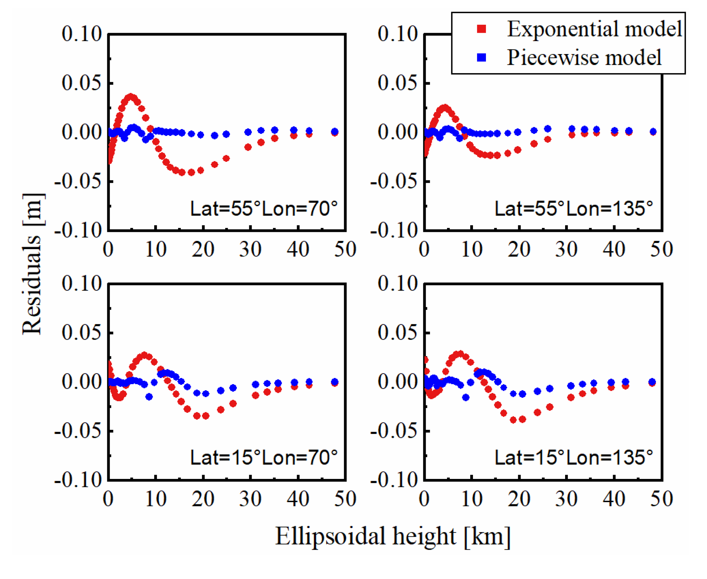
Figure 3 shows the comparison between residuals of the exponential model and the piecewise model on fitting the ERA5 ZTD atmospheric profile of four different grid points at UTC 0:00 on 1 January 2013. From Figure 3, we can know that the piecewise model has a better performance on fitting. For better comparison, the fitting residuals of ERA5 ZTD atmospheric profile at all grids during the period of 2013–2018 are also computed. The mean root-mean-square (RMS) of residuals of the exponential model and the piecewise model is 1.64 cm and 0.32 cm, respectively. Compared to the exponential model, the mean RMS of residuals can be improved by about 80.5% with the piecewise model.
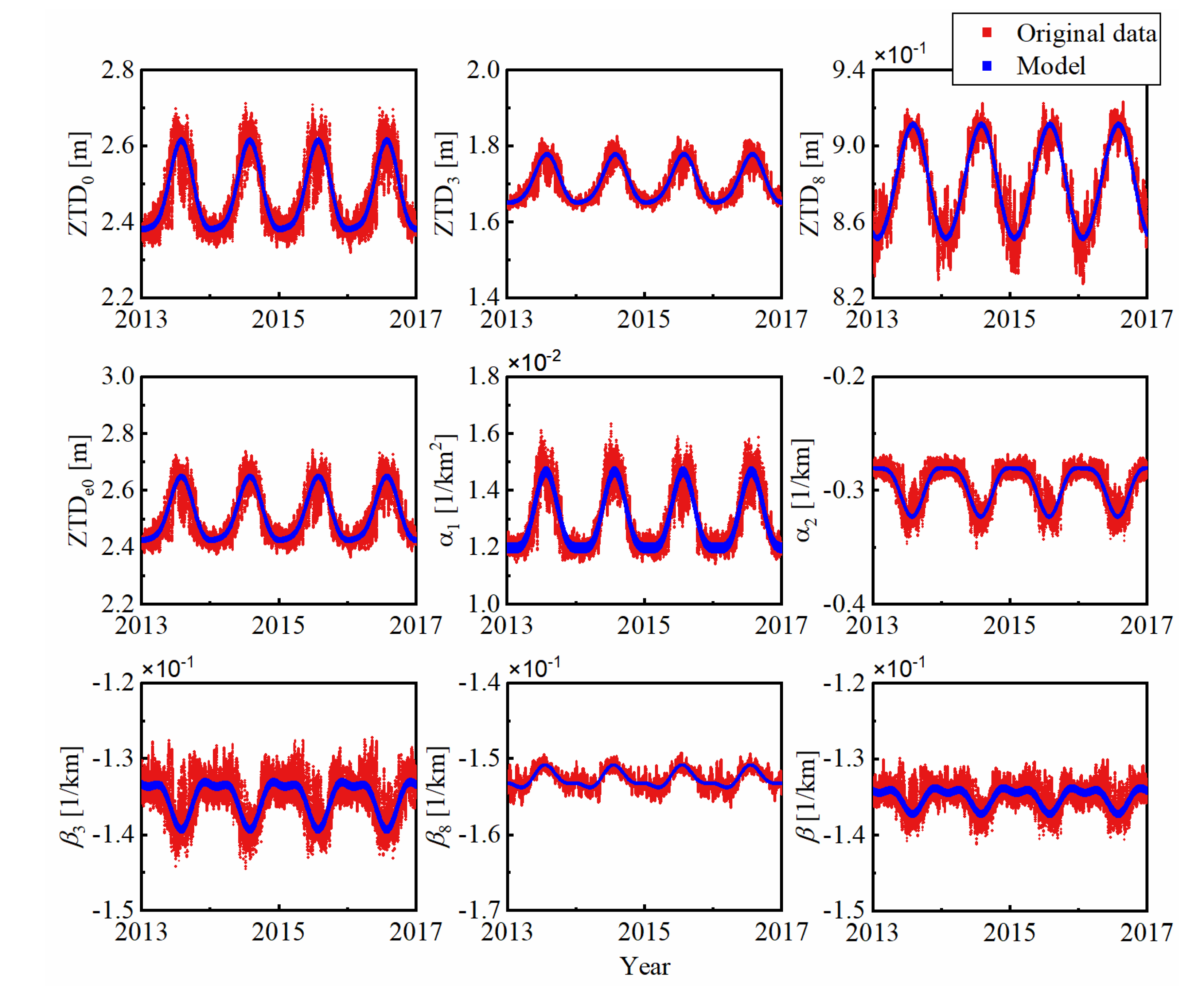
Based on the time series of ZTD derived from the aforementioned ERA5 regional reanalysis data in 2013–2017, we can calculate the unknown model coefficients in Equations (13) and (15) at each grid point using the least-square method. Figure 4 shows the performance of the trigonometric function on fitting the unknown parameters of the exponential model and the piecewise model. From Figure 4, we know that the parameters obtained by Equations (13) and (15) are close to the original data estimated by Equations (12) and (14), which indicates that the trigonometric function can better reflect the periodic variation of the estimated parameters.
These model coefficients estimated by Equation (13) are stored as grids with a resolution of 2.5° × 2.5° on longitude and latitude, respectively. If a station is not on the grid point, the corresponding model coefficients can be obtained using the surrounding grid points with the bilinear interpolation scheme. With the model coefficients of trigonometric function stored at each grid point, the RGZTD model (using the piecewise model) is established. For comparison, we use the same strategy as the RGZTD model to establish the exponential model (using the exponential model).

4. Model Validation

To verify the performance of RGZTD model, the ZTD data derived from ERA5 reanalysis data, radiosonde data and CMONOC data were used as well as the other three empirical ZTD models: Exponential model, UNB3M model and GPT3 model (1° × 1°) were compared. In this study, the output pressure, water vapor pressure, weighted mean temperature and water vapor decrease factor by the GPT3 model at a certain time and ellipsoidal height are used to calculate the ZTD data of GPT3 model. With these output values, the zenith hydrostatic delay (ZHD) can be determined with the Saastamoinen model, which is shown as follows:
ZHD = 0.0022768 × P 1 0.00266 cos 2 φ 0.00028 h
and the zenith wet delay (ZWD) is calculated using the formula by [27]:
ZWD = 10 6 ( k 2 + k 3 T m ) R d e g 0 ( λ + 1 )
where k 2 = 16.52 K/hPa, Tm is the weighted mean temperature (K), Rd = 287.0464 JK−1 kg−1, which is the specific gas constant for dry constituents.
We use the mean bias and RMS to evaluate the model performance of the proposed new method. They are calculated by:
B i a s = 1 n i = 1 n ( X i X t r u e )
R M S = 1 n i = 1 n ( X i X t r u e ) 2
where Xi is the model-derived ZTD value and Xtrue is the ZTD value from ERA5 reanalysis data, or radiosonde data, or CMONOC data.

4.1. Accuracy Analysis Based on ERA5 ZTD Data

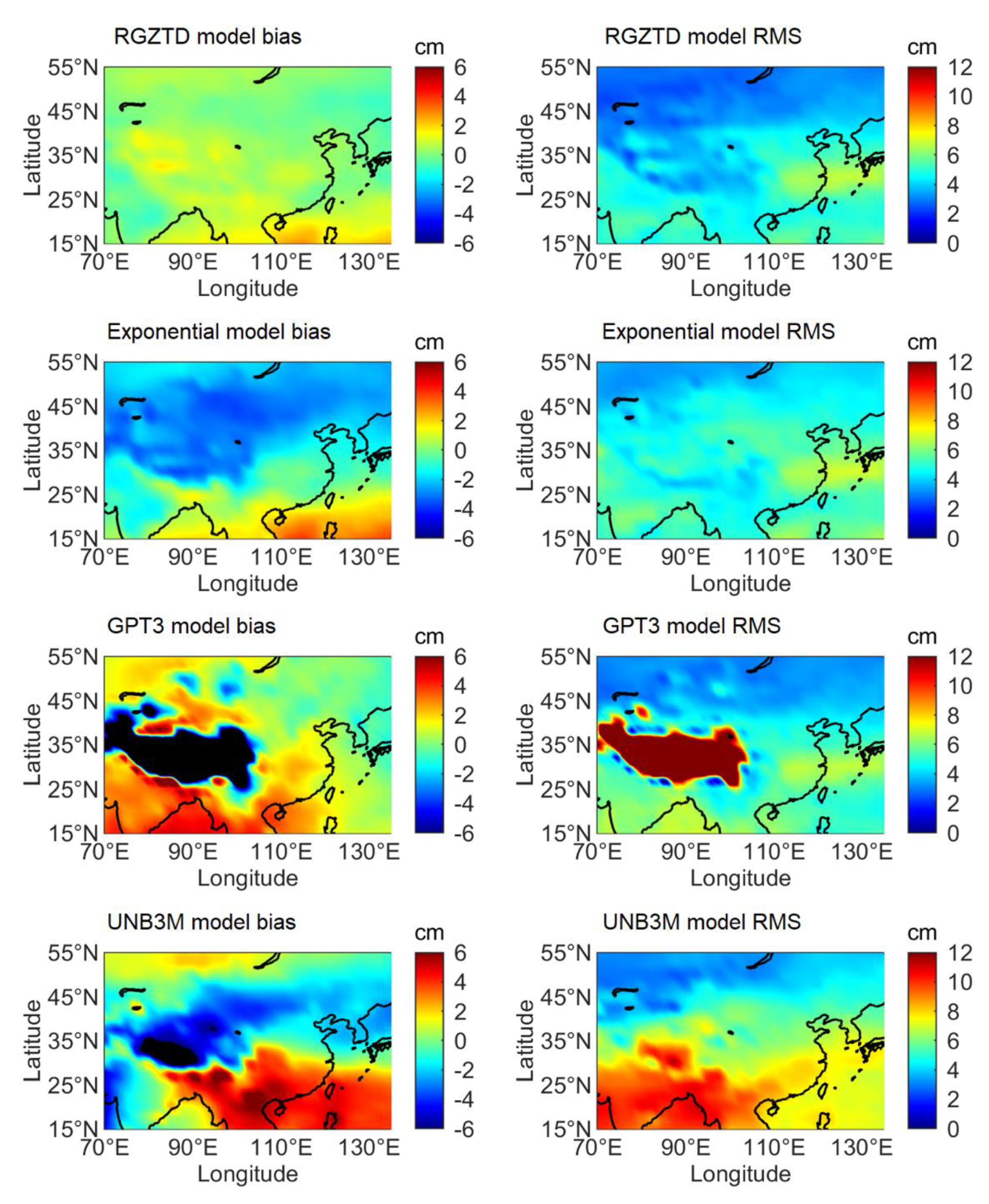
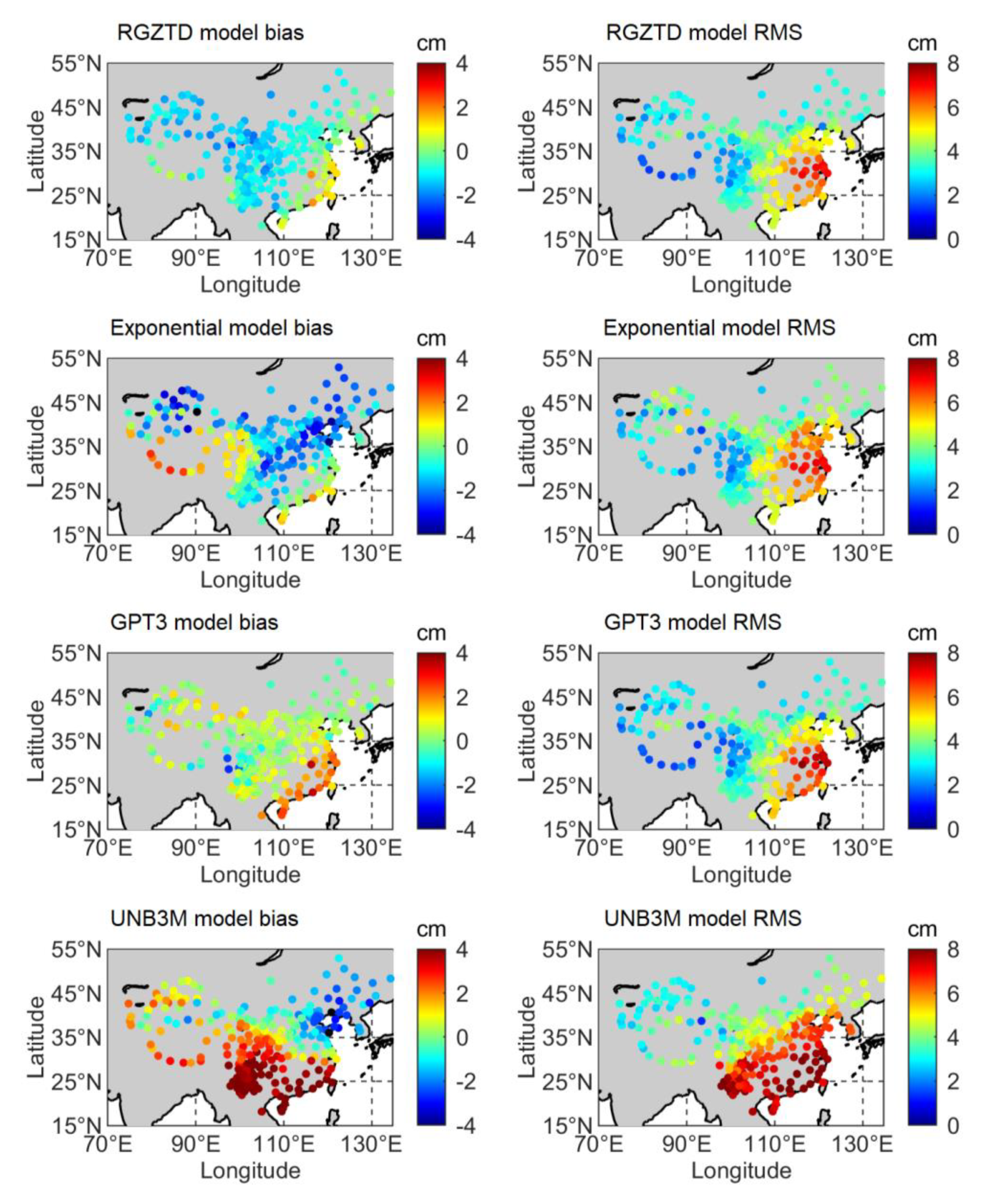
The ERA5 ZTD data at the height corresponding to bottom pressure level (1000 hPa) during the period of 2017–2018 is considered as reference for verifying the accuracy of the RGZTD model. Figure 5 shows the bias and RMS values of RGZTD model, Exponential model, UNB3M model and GPT3 model adopting the ERA5 ZTD data as reference. Figure 5 illustrates that the bias of RZTD model is more uniform and closer to zero comparing with that of other models. The RMS distribution of RGZTD model is similar with that of Exponential model. Moreover, the overall RMS of RGZTD model is less than that of Exponential model. Except for Tibet Plateau, the RMS distribution of GPT3 model is relatively uniform. The reason may be that the height corresponding to ERA5 bottom pressure level is far from the surface in the Tibet Plateau and the altitude variation of ZTD cannot be well described by GPT3 model. For UNB3M model, the overall RMS is larger than that of RZTD model or Exponential mode. Further, the UNB3M model has a poor accuracy at low latitude and coastal areas, which may be affected by land-sea distribution, temperature variation and the defects of the model itself [16].
Validation results from the four models are given in Table 1. In Table 1, we calculate the mean bias and RMS over China and the surrounding areas. The mean biases of RGZTD model, Exponential model, GPT3 model and UNB3M model are 0.38 cm, −1.24 cm, −1.52 cm and 0.04 cm, respectively. Moreover the mean RMSs of RGZTD model, exponential model, GPT3 model and UNB3M model are 4.18 cm, 4.83 cm, 7.11 cm, and 6.39 cm, respectively. The mean biases of RGZTD model and UNB3M model are close to zero and the overall estimates are larger than reference values. The mean biases of the exponential model and GPT3 model are within 2 cm and the overall estimates are less than reference values. Because of the poor-fitting effect in vertical direction in Tibet Plateau, the accuracy of the GPT3 model is worse than other models. The accuracy of the GZTD model is the third. Compared with that of Exponential model, the accuracy of calculated ZTD can be improved by about 13.4% with RGZTD model. The difference shows itself as the better accuracy results of RGZTD model than that of the exponential model.

4.2. Accuracy Analysis Based on Radiosonde ZTD Data

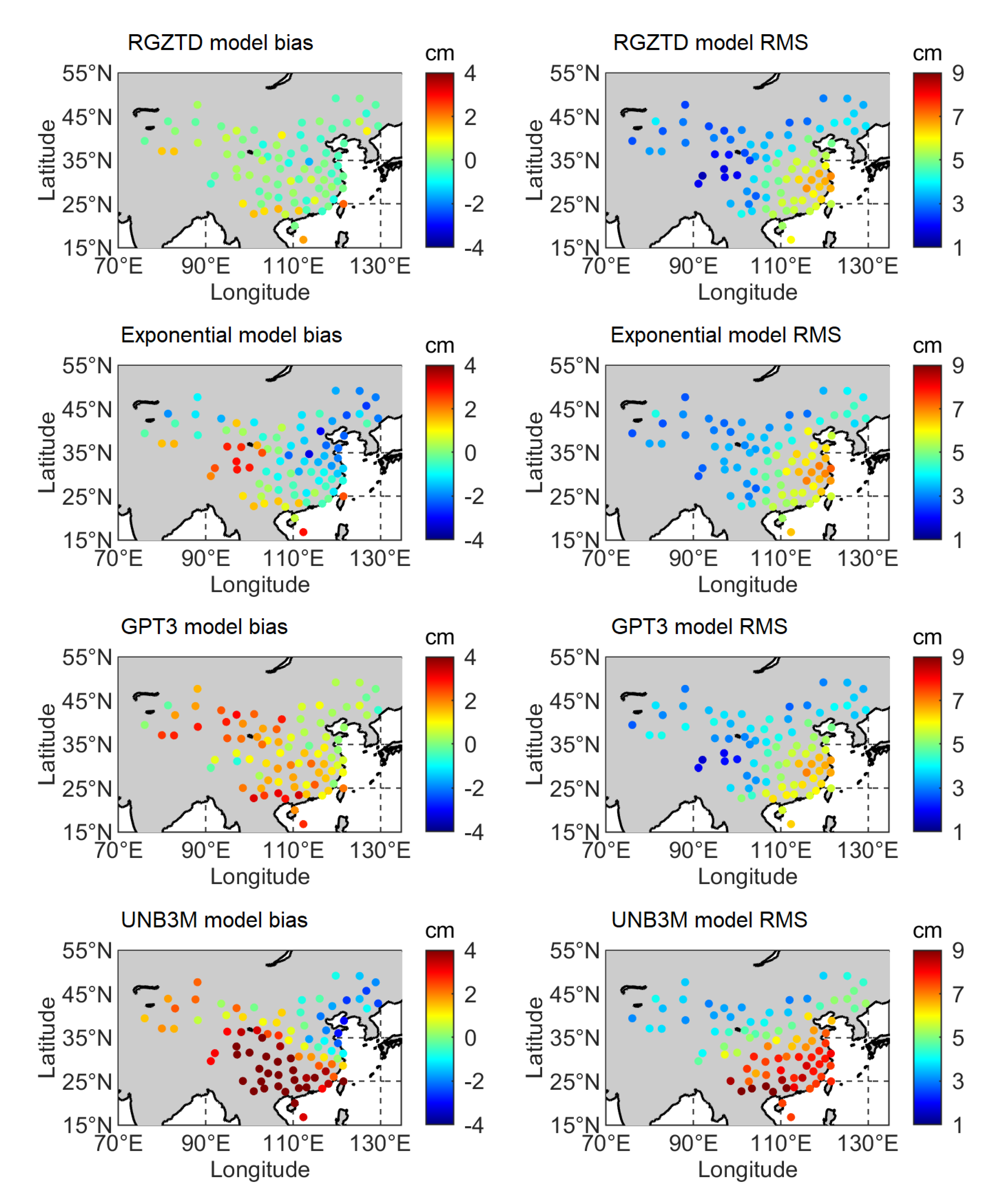
In order to verify the accuracy and reliability of RGZTD model, the ZTD derived from radiosonde data on 86 stations in China from 2017–2018 was used as another reference. Figure 6 shows the bias and RMS values of RGZTD model, Exponential model, GPT3 model and UNB3M model when the radiosonde ZTD data are compared. In Figure 6, we can find that the overall bias of RZTD model is close to zero, and most of them are within 2 cm. The biases of the exponential model and GPT3 model change from negative to positive with the changes of the station locations from coastal areas to inland areas. For the UNB3M model, the biases change from positive to negative with the increasing latitude. Additionally, the overall RMSs of coastal areas of four models are larger than those of inland areas.
Table 2 shows the mean bias and RMS of four models on 86 radiosonde stations. The mean biases of RGZTD model, Exponential model, GPT3 model and UNB3M model are 0.07 cm, −0.32 cm, 1.30 cm and 1.89 cm, respectively. The ZTD estimate of Exponential model is less than the reference value while the ZTD estimates of RGZTD model, GPT3 model and UNB3M model are larger than reference values. Moreover, the mean RMSs of the RGZTD model, exponential model, GPT3 model, and UNB3M model are 4.19 cm, 4.51 cm, 4.46 cm, and 6.02 cm, respectively. The accuracy of UNB3M model is the worst while RGZTD model has similar accuracy with GPT3 model. Compared with that of Exponential model, the accuracy of calculated ZTD can be improved by about 7.1% with the RGZTD model. When the radiosonde ZTD data are used as the reference value, RGZTD model has better performance if the exponential model is compared.

4.3. Accuracy Analysis Based on CMONOC Tropospheric Products

With the development of GNSS, it has proved to be a powerful tool in navigation, positioning, and measuring atmospheric water vapor [28]. Thus, the tropospheric products from 251 CMONOC GNSS stations are used as the third reference values to verify the accuracy and reliability of RGZTD model. Because there are some gross errors in CMONOC tropospheric products during the period of 2017–2018, the ZTD data derived from the products in 2016–2017 is used in this study. Figure 7 shows the bias and RMS values of RGZTD model, Exponential model, GPT3 model and UNB3M model when the CMONOC ZTD data are compared. From Figure 7, we can find that most of the biases of RGZTD model and GPT3 model are close to zero and range from −1 cm to 1 cm. In addition to southeast coastal areas, the bias distribution is uniform in other areas. For the exponential model, the biases in Tibet Plateau and southeast coastal areas are larger than other areas. Moreover, UNB3M model has larger bias in low latitude areas. In addition, the RMS distributions of the four models are similar. In southeast coastal areas, the tropospheric delays estimated by the four models are larger than reference values.
Table 3 shows the mean biases and RMSs of four models over China’s 251 CMONOC stations. The mean biases of RGZTD model, Exponential model, GPT3 model and UNB3M model are −0.81 cm, −0.97 cm, 0.42 cm and 1.31 cm, respectively. UNB3M model has largest absolute value of the mean bias. The absolute values of biases of other three model are within 1 cm. The mean RMSs of RGZTD model, Exponential model, GPT3 model and UNB3M model are 3.76 cm, 4.01 cm, 3.74 cm, and 5.42 cm, respectively. RGZTD model and GPT3 model have similar accuracy. The accuracy of UNB3M model is the worst. Compared with that of the exponential model, the accuracy of calculated ZTD can be improved by about 6.2% with RGZTD model.

5. Conclusions

It is important to obtain high-accuracy ZTD data for GNSS positioning and water vapor retrieval, especially for some GNSS receivers not equipped with collocated meteorological sensors. In recent years, many empirical models without any meteorological parameters, largely based on data from radiosondes, or an NWP model’s output, or atmospheric reanalysis products, or GNSS tropospheric products, have been built. To describe the variation of ZTD in vertical direction, the coarse exponential model is often used based on the relationship between altitude and ZTD value. In fact, ZTD is derived by integrating the atmospheric refractivity at different heights. A new model can also be obtained by integrating the model that describes the relationship between atmospheric refractivity and height.
In this study, we provide a new modeling method for the ZTD empirical model, which is based on the piecewise model of atmospheric refractivity. Compared with the exponential model, the adjusted piecewise model has a better performance in fitting the ZTD data in vertical direction. With the ZTD data derived from ERA5 hourly 2.5° × 2.5° pressure level data during the period of 2013–2017, we establish a new regional gridded ZTD model (RGZTD), ranging from 70° E to 135° E in longitude and from 15° N to 55° N in latitude. Further, the model coefficients of the RGZTD model are stored as grids with a resolution of 2.5° × 2.5° on longitude and latitude, respectively. Thus, the latitude, longitude, ellipsoidal height, and day of year are needed as the input data. To verify the validation and accuracy of RGZTD model, the ZTD data derived from ERA5 reanalysis data, radiosonde data and GNSS data in CMONOC were used. Results show that the mean absolute bias of RGZTD model is within 1 cm. Moreover, the accuracy can be improved by about 13.4%, 7.1%, and 6.2% when ERA5 reanalysis data, radiosonde data, and CMONOC data are used as reference values, respectively. The difference shows the more accurate results of the RGZTD model in comparison to the exponential model.
This study mainly focuses on a new ZTD modeling method (piecewise model in vertical direction) and proposes a regional gridded ZTD model (RGZTD model). In addition to the horizontal refraction gradient that is also important in determining the atmospheric delay, the previous model can be used when it is needed. In addition, there are obvious systematic biases in different data sets in the process of model validation. Determining the systematic bias and establishing a better ZTD empirical model based on multisource data fusion should be paid more attention in future studies.

Author Contributions

Data curation, L.Y., D.Z. and Z.L.; formal analysis, L.Y., J.G., D.Z., N.Z. and Z.L.; methodology, L.Y.; writing—original draft, L.Y. and N.Z.; writing—review & editing, L.Y., J.G., D.Z., N.Z. and Z.L. All authors have read and agreed to the published version of the manuscript.

Funding

This research was funded by the National Natural Science Foundation of China (No. 41974039, No. 41674008, No. 41974026 and No. 4P184081).

Acknowledgments

The authors are also grateful for the ERA5 reanalysis produced by ECMWF, the radiosonde provided by University of Wyoming and the CMONOC tropospheric products produced by GNSS data product service platform of China Earthquake Administration.

Conflicts of Interest

The authors declare no conflict of interest.

References

  1. Penna, N.; Dodson, A.; Chen, W. Assessment of EGNOS tropospheric correction model. J. Navig. 2001, 54, 37–55. [Google Scholar] [CrossRef] [Green Version]
  2. Zheng, F.; Lou, Y.; Gu, S.; Gong, X.; Shi, C. Modeling tropospheric wet delays with national GNSS reference network in China for BeiDou precise point positioning. J. Geod. 2018, 92, 545–560. [Google Scholar] [CrossRef]
  3. Black, H.D. An easily implemented algorithm for the tropospheric range correction. J. Geophys. Res. Solid Earth 1978, 83, 1825–1828. [Google Scholar] [CrossRef]
  4. Hopfield, H.S. Two-quartic tropospheric refractivity profile for correcting satellite data. J. Geophys. Res. (1896–1977) 1969, 74, 4487–4499. [Google Scholar] [CrossRef]
  5. Saastamoinen, J. Atmospheric correction for troposphere and stratosphere in radio ranging of satellites. In Proceedings of the 3rd Int Symp on the Use of Artificial Satellites for Geodesy, Washington, DC, USA, 15–17 April 1972. [Google Scholar]
  6. Collins, J.P.; Langley, R.B. A Tropospheric Delay Model for the User of the Wide Area Augmentation System; Department of Geodesy and Geomatics Engineering, University of New Brunswick: Fredericton, NB, Canada, 1997. [Google Scholar]
  7. Collins, P.; Langley, R.; LaMance, J. Limiting factors in tropospheric propagation delay error modelling for GPS airborne navigation. In Proceedings of the 52nd ION Annual Meeting, Cambridge, MA, USA, 19–21 June 1996; Volume 3. [Google Scholar]
  8. Ueno, M.; Hoshinoo, K.; Matsunaga, K.; Kawai, M.; Nakao, H.; Langley, R.B.; Bisnath, S.B. Assessment of atmospheric delay correction models for the Japanese MSAS. In Proceedings of the 14th International Technical Meeting of the Satellite Division of The Institute of Navigation (ION GPS 2001), Salt Lake City, UT, USA, 11–14 September 2001; pp. 2341–2350. [Google Scholar]
  9. Li, W.; Yuan, Y.; Ou, J.; He, Y. IGGtrop_SH and IGGtrop_rH: Two Improved Empirical Tropospheric Delay Models Based on Vertical Reduction Functions. IEEE Trans. Geosci. Remote Sens. 2018, 56, 5276–5288. [Google Scholar] [CrossRef]
  10. Li, W.; Yuan, Y.; Ou, J.; Li, H.; Li, Z. A new global zenith tropospheric delay model IGGtrop for GNSS applications. Chin. Sci. Bull. 2012, 57, 2132–2139. [Google Scholar] [CrossRef] [Green Version]
  11. Yao, Y.; Hu, Y.; Yu, C.; Zhang, B.; Guo, J. An improved global zenith tropospheric delay model GZTD2 considering diurnal variations. Nonlinear Process. Geophys. 2016, 23, 127–136. [Google Scholar] [CrossRef] [Green Version]
  12. Yao, Y.-B.; He, C.-Y.; Zhang, B.; Xu, C.-Q. A new global zenith tropospheric delay model GZTD. Chin. J. Geophys. Chin. Ed. 2013, 56, 2218–2227. [Google Scholar] [CrossRef]
  13. Schueler, T. The TropGrid2 standard tropospheric correction model. Gps Solut. 2014, 18, 123–131. [Google Scholar] [CrossRef]
  14. Dousa, J.; Elias, M. An improved model for calculating tropospheric wet delay. Geophys. Res. Lett. 2014, 41, 4389–4397. [Google Scholar] [CrossRef]
  15. Sun, J.; Wu, Z.; Yin, Z.; Ma, B. A simplified GNSS tropospheric delay model based on the nonlinear hypothesis. Gps Solut. 2017, 21, 1735–1745. [Google Scholar] [CrossRef]
  16. Chen, P.; Ma, Y.; Liu, H.; Zheng, N. A New Global Tropospheric Delay Model Considering the Spatiotemporal Variation Characteristics of ZTD With Altitude Coefficient. Earth Space Sci. 2020, 7. [Google Scholar] [CrossRef]
  17. Li, L.; Xu, Y.; Yan, L.; Wang, S.; Liu, G.; Liu, F. A Regional NWP Tropospheric Delay Inversion Method Based on a General Regression Neural Network Model. Sensors 2020, 20, 3167. [Google Scholar] [CrossRef] [PubMed]
  18. Charoenphon, C.; Satirapod, C. Improving the accuracy of real-time precipitable water vapour using country-wide meteorological model with precise point positioning in Thailand. J. Spat. Sci. 2020. [Google Scholar] [CrossRef]
  19. Chen, J.; Wang, J.; Wang, A.; Ding, J.; Zhang, Y. SHAtropE-A Regional Gridded ZTD Model for China and the Surrounding Areas. Remote Sens. 2020, 12, 165. [Google Scholar] [CrossRef] [Green Version]
  20. Boehm, J.; Moeller, G.; Schindelegger, M.; Pain, G.; Weber, R. Development of an improved empirical model for slant delays in the troposphere (GPT2w). GPS Solut. 2015, 19, 433–441. [Google Scholar] [CrossRef] [Green Version]
  21. Landskron, D.; Boehm, J. VMF3/GPT3: Refined discrete and empirical troposphere mapping functions. J. Geod. 2018, 92, 349–360. [Google Scholar] [CrossRef]
  22. Albergel, C.; Dutra, E.; Munier, S.; Calvet, J.-C.; Munoz-Sabater, J.; de Rosnay, P.; Balsamo, G. ERA-5 and ERA-Interim driven ISBA land surface model simulations: Which one performs better? Hydrol. Earth Syst. Sci. 2018, 22, 3515–3532. [Google Scholar] [CrossRef] [Green Version]
  23. Hersbach, H.; Dee, D. ERA5 Reanalysis Is in Production. Available online: https://www.ecmwf.int/en/newsletter/147/news/era5-reanalysis-production (accessed on 17 October 2020).
  24. Ge, S. GPS Radio Occultation and the Role of Atmospheric Pressure on Spaceborne Gravity Estimation over Antarctica. Ph.D. Thesis, The Ohio State University, Columbus, OH, USA, 2006. [Google Scholar]
  25. Salamon, S.J.; Hansen, H.J.; Abbott, D. Modelling radio refractive index in the atmospheric surface layer. In Electronics Letters; Institution of Engineering and Technology: London, UK, 2015; Volume 51, pp. 1119–1121. [Google Scholar]
  26. Bean, B.R.; Thayer, G.D. Models of the Atmospheric Radio Refractive Index. Proc. IRE 1959, 47, 740–755. [Google Scholar] [CrossRef]
  27. Askne, J.; Nordius, H. Estimation of tropospheric delay for microwaves from surface weather data. Radio Sci. 1987, 22, 379–386. [Google Scholar] [CrossRef]
  28. Huang, L.; Jiang, W.-P.; Liu, L.; Chen, H.; Ye, S. A new global grid model for the determination of atmospheric weighted mean temperature in GPS precipitable water vapor. J. Geod. 2018. [Google Scholar] [CrossRef]
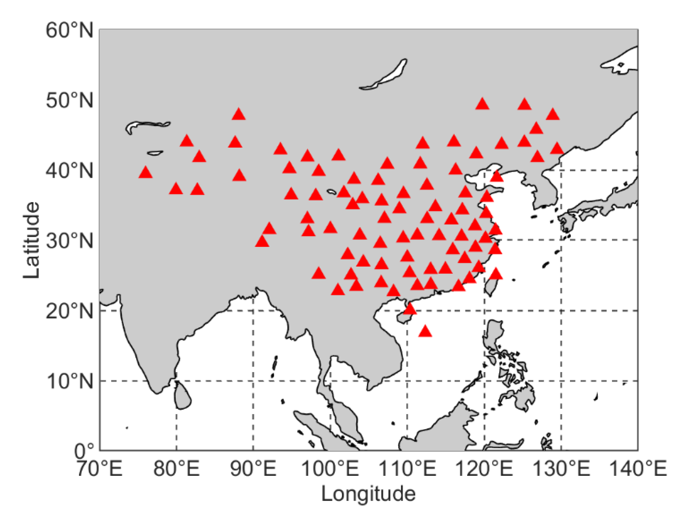
Figure 1. Geographic distribution of the 86 radiosonde stations.
Remotesensing 12 03876 g001
Figure 2. Geographic distribution of the 251 GNSS stations.
Remotesensing 12 03876 g002
Figure 3. Fitting residuals of the exponential model and the piecewise model at different grid points.
Remotesensing 12 03876 g003
Figure 4. Comparison of estimated parameters (Original data) and results of spectral analysis (Model) at the grid point (longitude 100° and latitude 30°) in 2013–2017.
Remotesensing 12 03876 g004
Figure 5. Distribution of bias and RMS of RGZTD model, Exponential model, GPT3 model and UNB3M model over China and the surrounding areas, where the ERA5 ZTD data is the reference value.
Remotesensing 12 03876 g005
Figure 6. Distribution of bias and RMS of RGZTD model, Exponential model, GPT3 model and UNB3M model in China, where the radiosonde ZTD data is the reference value.
Remotesensing 12 03876 g006
Figure 7. Distribution of bias and RMS of RGZTD model, Exponential model, GPT3 model and UNB3M model in China, where the CMONOC ZTD data is the reference value.
Remotesensing 12 03876 g007
Table 1. Mean bias and RMS of RGZTD model, Exponential model, GPT3 model and UNB3M model with respect to ERA5 ZTD data in 2017–2018 [cm].
Mean of BiasMean of RMS
RGZTD model0.384.18
Exponential model−1.244.83
GPT3 model−1.527.11
UNB3M model0.046.39
Table 2. Mean bias and RMS of RGZTD model, Exponential model, GPT3 model with respect to radiosonde ZTD data in 2017–2018 [cm].
Mean of BiasMean of RMS
RGZTD model0.074.19
Exponential model−0.324.51
GPT3 model1.304.46
UNB3M model1.896.02
Table 3. Mean bias and RMS of RGZTD model, Exponential model, GPT3 model and UNB3M model with respect to CMONOC ZTD data in 2016–2017 [cm].
Mean of BiasMean of RMS
RGZTD model−0.813.76
Exponential model−0.974.01
GPT3 model0.423.74
UNB3M model1.315.42
Publisher’s Note: MDPI stays neutral with regard to jurisdictional claims in published maps and institutional affiliations.