Article

RCSANet: A Full Convolutional Network for Extracting Inland Aquaculture Ponds from High-Spatial-Resolution Images

1
College of Oceanography and Space Informatics, China University of Petroleum, Qingdao 266580, China
2
State Key Laboratory of Information Engineering in Surveying, Mapping and Remote Sensing, Wuhan University, Wuhan 430079, China
3
Key Laboratory for Geographical Process Analysis & Simulation of Hubei Province, College of Urban and Environmental Sciences, Central China Normal University, Wuhan 430079, China
4
Key Laboratory of Algal Biology, Institute of Hydrobiology, Chinese Academy of Sciences, Wuhan 430072, China
5
NavInfo Co., Ltd., Beijing 100094, China
*
Author to whom correspondence should be addressed.
Remote Sens. 2021, 13(1), 92; https://doi.org/10.3390/rs13010092
Submission received: 10 December 2020 / Revised: 25 December 2020 / Accepted: 26 December 2020 / Published: 30 December 2020
(This article belongs to the Special Issue Remote Sensing of the Aquatic Environments)

Abstract

:
Numerous aquaculture ponds are intensively distributed around inland natural lakes and mixed with cropland, especially in areas with high population density in Asia. Information about the distribution of aquaculture ponds is essential for monitoring the impact of human activities on inland lakes. Accurate and efficient mapping of inland aquaculture ponds using high-spatial-resolution remote-sensing images is a challenging task because aquaculture ponds are mingled with other land cover types. Considering that aquaculture ponds have intertwining regular embankments and that these salient features are prominent at different scales, a Row-wise and Column-wise Self-Attention (RCSA) mechanism that adaptively exploits the identical directional dependency among pixels is proposed. Then a fully convolutional network (FCN) combined with the RCSA mechanism (RCSANet) is proposed for large-scale extraction of aquaculture ponds from high-spatial-resolution remote-sensing imagery. In addition, a fusion strategy is implemented using a water index and the RCSANet prediction to further improve extraction quality. Experiments on high-spatial-resolution images using pansharpened multispectral and 2 m panchromatic images show that the proposed methods gain at least 2–4% overall accuracy over other state-of-the-art methods regardless of regions and achieve an overall accuracy of 85% at Lake Hong region and 83% at Lake Liangzi region in aquaculture pond extraction.

Graphical Abstract

1. Introduction

Aquaculture has become one of the main sources of animal protein and increasingly contributes to food security for many inland cities with large populations in Asia. Freshwater aquaculture products such as fish, crustaceans, and molluscs are supplied from aquaculture ponds built around natural lakes. Aquaculture in China already accounts for 60% of global production [1]. Aquaculture foods provided by inland aquaculture ponds have become predominant contributors of aquatic foods in Chinese banquets [2]. Provinces in the middle and lower reaches of the Yangtze River basin account for more than half the country’s total freshwater production. In recent years, pond aquaculture has become predominant and has contributed on average 71 percent to total freshwater production (China Fishery Statistical Yearbook 2004–2016), maintaining an average growth rate of 5.8 percent per year. The area under pond aquaculture has greatly increased. However, intensive aquaculture has a severely destructive effect on the environment, including high levels of water use, local environmental pollution, and the loss of services provided by the freshwater ecosystems of natural lakes [3,4].
Remotely sensed imagery has been used as an effective means for global monitoring of aquaculture ponds in coastal areas [5,6,7] and nearby inland lakes [8]. An object-based image analysis (OBIA) method was used on Landsat TM images to extract aquaculture ponds in coastal areas of south-eastern China [9]. Tran et al. used maximum likelihood classification on Landsat and SPOT5 images to obtain long-term land-cover and land-use changes in a delta in Vietnam, where aquaculture ponds were one of the classes [10]. Ottinger et al. used the geometric features of aquaculture ponds for image segmentation on Sentinel-1 Synthetic Aperture Radar (SAR) images to extract fish ponds in several delta areas in Asia [5,11]. Zeng et al. used Landsat and Gaofen-1 satellite images to extract aquaculture ponds around inland lakes using boundary curve features and a Support Vector Machine (SVM) classifier [8]. In state-of-the-art methods for aquaculture pond extraction, object-oriented classification is usually integrated with hand-crafted features, and the spatial resolution of the satellite images commonly used is generally 10 meters or coarser. However, aquaculture ponds close to inland lakes are mixed with water bodies that are approximately the same size as these ponds. Accurately mapping aquaculture ponds using finer spatial resolution (up to a few meters) remote-sensing images and applying a more generalized approach, rather than manual feature engineering, remains a technical challenge for inland lake mapping.
Because semantic segmentation can understand images at the pixel level, statistics- and geometry-based image segmentation methods have been replaced by methods that depend on Deep Convolutional Neural Networks (DCNNs) [12]. DCNNs have been recognized by industry and have become widely used, advancing from LeNet-5’s success in zip encoding recognition in the 1980s to AlexNet’s victory in the 2012 ImageNet competition [13]. Subsequently, a deep CNN architecture proposed by Visual Geometry Group of Oxford University (VGG) [14], a residual network architecture proposed by He (ResNet) [15] and other DCNN structures have become the basic learning framework for advanced feature extraction from visual images. The fully convolutional network (FCN) constitutes a breakthrough in semantic image segmentation by converting the fully connected layer in traditional DCNNs, such as VGG, into a fully convolutional layer, thereby successfully achieving end-to-end labelling [16]. Badrinarayanan et al. [17] proposed Segnet to achieve pixel level classification through a deep convolutional encoder-decoder architecture in which the decoder upsamples the lower-resolution feature maps. Chen et al. proposed the Deeplab architecture and its revised versions, which introduced atrous convolution and atrous spatial pyramid pooling (ASPP) models into the deep encoder-decoder architecture for semantic segmentation [18,19,20]. Deep learning techniques for semantic segmentation have been developed for various computer vision tasks such as autonomous vehicles, medical research and many other applications in recent years [21]. However, implementing semantic segmentation of deep neural networks on remote-sensing images must overcome specific problems, including different data sources and scales [22]. For example, SegNet and ResNet have been efficiently implemented on multi-modal remote-sensing data using the FuseNet principle [23]. FCN has been used for slum mapping by transfer learning [24]. FCN was re-designed and used for automatic raft labelling in offshore waters by a dual-scale structure [25] or a U-Net [26].
Aquaculture ponds are shallow artificial water bodies that commonly have distinctly man-made shapes for efficient aquaculture production [10]. The ponds around inland lakes are formed gradually by embankment, partition, and regularization of other land cover types, such as cropland or natural lake water bodies. Because the shoreline of a natural lake winds along the surrounding terrain, its boundary shape is generally extremely irregular. On the other hand, the borders of aquaculture ponds are constructed on the principle of cost-saving, and straight lines are often used to delimit the boundary in a local area. Hence, the boundaries of aquaculture ponds have more regular shapes overall. Furthermore, when the human eye perceives satellite images where aquaculture ponds are densely distributed, the aquaculture ponds with their intertwining regular boundaries will be visual attention areas because human perception commonly pays attention to parts of visual space where patterns can be acquired, according to neuroscience and cognitive science literature [27].
Attention mechanisms have been extensively used for various visual tasks. The recurrent attention model is used for object recognition through a recurrent neural network (RNN) integrated with reinforcement learning to mimic the process of the human visual system as it recurrently determines the attention region. The attention mechanism on top of the RNN proposed by the neural machine translation community [28,29], was also adopted to perform image captioning by assigning different weights to image representations [30]. The self-attention mechanism without the RNN model is exploited in a super-resolution image generator [31], which is a variant of the TRANSFORMER [32], a cutting-edge deep neural network for language translation. Furthermore, self-attention mechanisms have been introduced into scene segmentation for modelling feature dependencies from spatial and channel dimensions [33]. In remote sensing, attention models have also been used for object classification in various satellite images. For instance, attention mechanisms are integrated into multi-scale and feedback strategies of deep neural networks for pixel-wise classification of very-high-resolution satellite images [34]. The attention model is combined with a learning layer to capture class-specific feature dependencies [35].
When human beings visually identify densely distributed aquaculture ponds on remote-sensing images, the intertwining regular embankments around these ponds are prominent visual attention features. This paper is inspired by this visual attention mechanism used for human interpretation of satellite images. Moreover, the intertwining regular embankments are a salient feature that is available at different scales. The two motivations of this study are first to develop a novel attention mechanism that can mimic the process of the human visual system to recurrently determine the attention region, which is the intertwining regular embankments of aquaculture ponds, and to evolve multi-scale visual attention through the encoder-decoder, fully convolutional network architecture that integrates the attention mechanism with atrous convolutions to better extract aquaculture ponds.
Therefore, the main contributions of the paper can be summarized as follows:
(1)
Propose the Row-wise and Column-wise Self-Attention (RCSA) mechanism, which can work in parallel to capture visual emphasis on salient pixels in the context of rows and columns from a remote-sensing image.
(2)
Propose an improved fully convolutional network based on the RCSA mechanism that is combined with an ASPP structure for multi-scale attention.
(3)
Evaluate the validity of the proposed method on a developed dataset that contains abundant aquaculture ponds around inland lakes.

2. Materials

2.1. Study Area

Hubei Province, known as the province of thousands of lakes, lies in the middle reaches of the Yangtze River and has densely distributed lakes. Hubei has a mature freshwater aquaculture industry with large numbers of aquaculture ponds developed surrounding natural lakes. As shown in Figure 1, six regions with densely distributed aquaculture ponds were selected as study areas from three large lakes (Lake Liangzi, Lake Futou, and Lake Hong) along the Yangtze River because these are typical inland aquaculture areas in China. Among them, Lake Hong and Lake Liangzi are the two largest freshwater lakes in Hubei Province. The population in this part of China is dense, and aquaculture is very developed. Lake Liangzi, and its surroundings, however, have been relatively well protected since the 1980s. The six selected regions were divided into two categories: type I and type II. The type I regions, including regions A and B, are used for testing, whereas type II regions are used for training. Region A is an area of 73.76 km2 close to eastern Lake Hong which is an artificial lake, and region B is an area of 33.92 km2 close to eastern Lake Liangzi, which has been preserved in a state more like a natural lake.

2.2. Dataset

The Landsat multispectral images were selected because of their long history. The bands such as the near infrared can be beneficial for extracting water bodies. However, the spatial resolution of Landsat multispectral data is only 30 m. Panchromatic images with 2–2.5 m spatial resolutions from the panchromatic and multispectral (PMS) camera of the GaoFen-1 (GF-1) satellite [36], the panchromatic remote-sensing instrument for stereo mapping (PRISM) of the ALOS satellite, and the NAD panchromatic sensor of the ZiYuan-3 (ZY-3) satellite [37] were also used to improve recognition and extraction of aquaculture ponds and natural water bodies. Table 1 lists the images used for the selected study regions. The Landsat multi-spectral images used in this study were captured in the winter of 2010–2011 and 2013–2014 and the spring of 2015. High-resolution panchromatic images were used for fusion with multi-spectral images. The panchromatic images were mainly selected from the GF-1 satellite and had acquisition dates close to the corresponding OLI images from Landsat satellite, whereas panchromatic images from the ALOS satellite were used instead for 2010 TM images from the Landsat satellite. However, when ALOS or GF-1 panchromatic images with similar acquisition dates were still not found, panchromatic images from the ZY-3 satellite captured in same season as Landsat images from a nearby year were selected because the ZY-3 satellite was launched in 2012.
Three classes: Aquaculture ponds (artificial water surfaces), natural water surfaces and background (non-water surfaces) were included in the reference dataset (Figure 1), which was mainly generated by human visual interpretation. Field investigations were also conducted on some difficult-to-identify features, in cases where aquaculture ponds were mixed with small natural water surfaces (Figure 2).

3. Methodology

To better understand the effectiveness of the proposed method for aquaculture pond segmentation, the methodology will be introduced in three parts: data pre-processing, the basic model, and a fusion strategy designed to further improve accuracy. In the preprocessing stage, the multi-spectral image and the corresponding 2 m panchromatic image were pansharpened. The pansharpened image was then fed into the proposed network, i.e., RCSANet, for semantic segmentation. The result generated from the network was finally fused with a water surface extraction image using the water index to further improve segmentation quality.

3.1. Preprocessing

Multi-spectral satellite images contain more spectral information, especially in the infrared spectral bands, which is beneficial for aquaculture pond identification, whereas panchromatic satellite images have higher spatial resolution, which helps to better distinguish the shape of the aquaculture pond. To use both together, the multi-spectral and high-spatial-resolution panchromatic images must be pansharpened to obtain images with both spectral information and higher spatial resolution. First, multi-spectral images were synthesized by selecting the three bands (green, red, NIR) that are useful for water body identification. The pixel values were normalized and then mapped to the range (0, 255). Similarly, the gray values of panchromatic images were also normalized and mapped to the range of (0, 255). The multi-spectral images were re-projected into the coordinate system of the corresponding panchromatic images to ensure consistent coordinates. The multi-spectral and panchromatic images were fused by the GRAM-SCHMIDT method [38], which is a widely used high-quality pansharpening method providing a fusion of panchromatic image and multi-spectral images with any number bands through orthogonalization of different multi-spectral bands [39].

3.2. Basic Model

3.2.1. Network Architecture

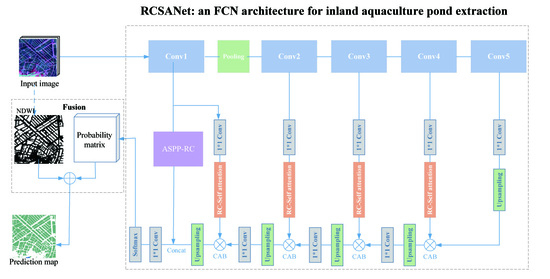
The deep neural network architecture, depicted in Figure 3a, for semantic segmentation of aquaculture ponds in the proposed method is based on an FCN framework, that uses ResNet-101 [15] as the encoder to generate multiple semantic features. The encoding part produces the feature maps through five convolution layers, including the first convolution layer (Conv1) followed by a pooling layer, and the other four convolution layers (Res-1 to Res-4) are all residual subnetworks. The feature maps are abstract representations of the input image at different levels. Semantic segmentation by the FCN framework is a dense prediction procedure in that the coarse outputs of the convolution layers are connected by upsampling to produce pixel-level prediction. In the proposed method, the RCSA mechanism (introduced in Section 3.2.2) was developed on the coarse outputs at different levels of abstract representation (detailed in Section 3.2.3). Next, channel attention blocks (CAB), which were designed to assign different weights to features at different stages for consistency [40], were used to connect the coarse abstract representations from the encoder with the upsampling feature at the decoder in the whole dense prediction procedure. The spatial size of the coarse outputs derived from the different convolution layers were kept consistent by the upsampling blocks (Figure 3c) to achieve end-to-end learning through backward propagation. Specifically, to accurately capture aquaculture ponds and their context information at multiple scales, the ASPP module combined with the RCSA mechanism (ASPP-RC) forms a branch from Conv1 to the end of the decoder before a 1 × 1 convolution layer and is integrated with the corresponding feature as a skip connection. To extract spatial context information at different scales, atrous convolutions with different rates, followed by the RCSA mechanism, were performed in parallel on the low-level feature map in the ASPP-RC module. These branches for capturing features at different scales are connected by weighting each branch in terms of its own importance (Figure 3b, introduced in Section 3.2.4).

3.2.2. RCSA Mechanism

When human beings use visual perception to understand remote-sensing images containing inland lakes with densely distributed aquaculture ponds, the ponds as a group will be eye-catching. The attention focuses on the spatial dependencies of aquaculture ponds and their surroundings. To mimic this human visual mechanism, the proposed model first establishes inter-pixel contextual dependencies through bidirectional gated recurrent units (GRUs) [41], which are a powerful variant of RNN, and then the self-attention modules are used on top of the bidirectional GRUs to establish this visual attention.
The self-attention mechanism is essentially a special case of the attention model. The unified attention model contains three types of inputs: key, value, and query [42], as depicted in Figure 4. The key and the value are a pair of data representations. Assume that there are T pairs < k i , v i > ( i 1 , , T ) . By evaluating the similarity between a query q and each key, the model essentially captures the weight coefficient of each key and then weights the corresponding values to derive their final attention values. The attention mechanism first scores the similarity between a query and a key pair by the f function:
e i = f ( k i , q )
Then the original scores e i are normalized by a Softmax function to obtain the weight coefficients:
a i = g ( e i ) = s o f t m a x ( e i ) = exp ( e i ) j = 1 T exp ( e j )
Finally, the context vector c t is evaluated by a weighted sum of the values:
c t = i a i v i
The attention model can be presented in a unified form
c t = A t t e n t i o n ( K , Q , V ) = S o f t m a x ( f ( K , q ) ) V
The attention model becomes a self-attention mechanism when all inputs, including the query, the key, and the value, have the same value.
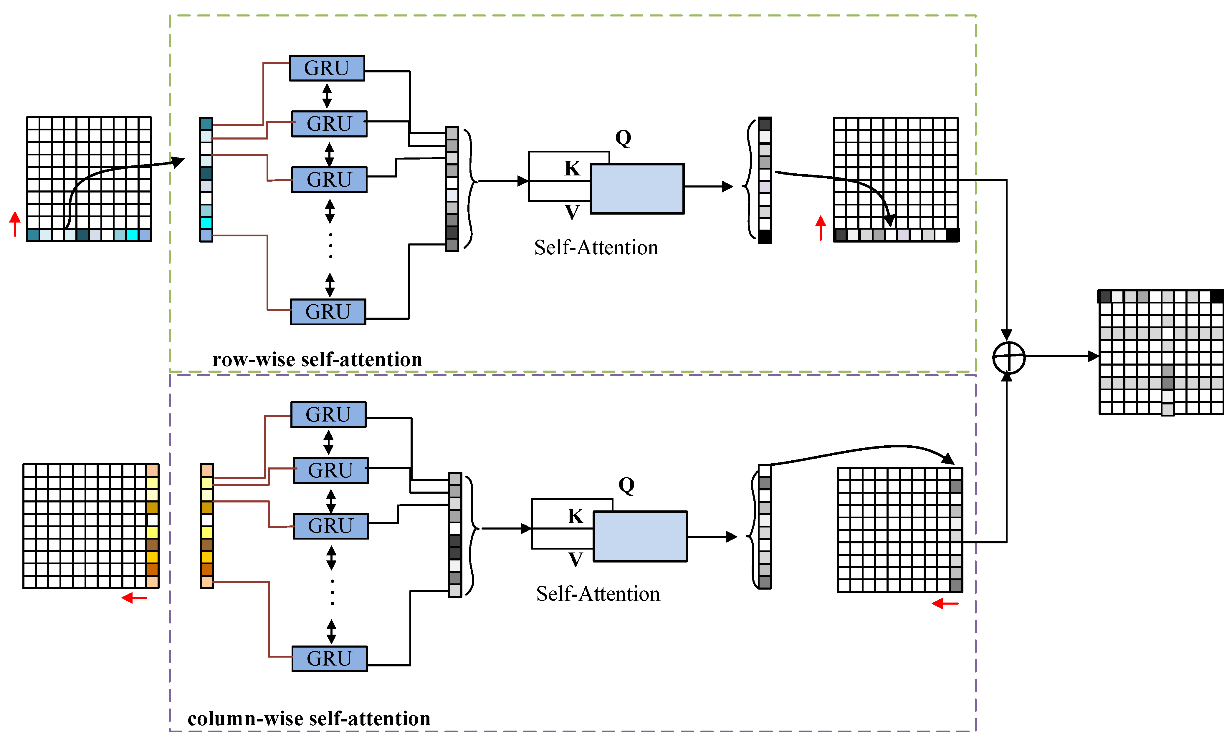
The RCSA mechanism takes a feature map, which is the convolutional result from the previous layer or the input image, as an input x R h × w × C , where h, w, and C are the number of rows, columns, and channels respectively. The feature map can be spatially divided into h rows r i R 1 × w × C ( i 1 h ) or w columns c j R h × 1 × C ( j 1 w ) . RCSA enables the construction of spatial dependencies between pixels within a row or a column by the self-attention mechanism. Hence, the RCSA mechanism consists of two parallel branches, column-wise and row-wise self-attention, which are subsequently concatenated by summation, as shown in detail in Figure 5. In the upper branch, the row-wise self-attention mechanism first uses the bidirectional GRU model to depict the dependencies between the pixels in a row of the feature map
r i = B i G R U ( r i )
Then the outcome from the GRUs r i is fed into the self-attention model by which the importance of the dependencies between pixels in the row is evaluated. The self-attention model is a specific variant of the attention model, in which the input query, key, and value have the same value, as shown in Figure 4b. The r i are respectively conducted by three 1 × 1 convolution kernels, W Q , W K ,and W V , so that the query, the key, and the value can be obtained by Q = W Q r i , K = W K r i , V = W V r i , where “*” is the convolution operation. Then they are substituted into the following Equation (4):
c t = A t t e n t i o n ( W K r i , W Q r i , W V r i ) = S o f t m a x ( f ( W K r i , W Q r i ) ) W V r i
where the similarity function f ( K , Q ) = Q K T d k and d k is the dimension of the key. The computation for one row can traverse to each row of the feature map. Equivalently, in the bottom branch, the same operations are performed in parallel on each column of the feature map. Eventually, the two branches are combined with equal weights.

3.2.3. RCSA for Dense Prediction

In semantic segmentation of remote-sensing images, dense prediction must fuse abstract representations of different levels from the encoder to improve pixel-level prediction. Visual attention on densely distributed aquaculture ponds could be involved in the dense prediction procedure. Consequently, the outputs of different convolution blocks in the encoding part are conducted by RCSA and then participate in dense prediction. These RCSA modules in the lateral connection enhance the features pixel-wise by assigning different weights to achieve a reasonable optimization of visual attention. In fact, this optimization takes place in a two-dimensional space made up of row and column vectors. However, the importance of different band channels must also be emphasized. The CAB module is directly used to fuse encoder and decoder features through assigning different weights to channels.

3.2.4. ASPP-RC Module

Atrous convolutions at different rates can enlarge the field of view so that spatial information at different scales can be extracted. Aquaculture ponds, which are water bodies surrounded by dikes with regular shapes, are densely distributed close to inland lakes. These features show visual salience in remote-sensing images. Hence, the RCSA block is arranged next to atrous convolution to selectively focus attention. After the first convolution blocks of the encoder, in the ASPP-RC module, the low-level feature map is executed in parallel by atrous convolutions with different rates combined with RCSA. Eventually, the branches are connected by:
I = i = 1 5 w i · b i
where b i is the feature map produced by the ith branch in which the atrous convolution and RCSA are conducted in sequence and w i is the weight of the ith branch that evaluates the importance of different scales. This is unlike the original ASPP structure in which each branch has the same importance. The importance of each branch is adjusted adaptively in the proposed ASPP-RC module. All weight parameters are initially defined by a random vector w i 0 , which can be optimized during backpropagation when training the whole network. Finally, these weights are normalized using a Softmax function:
w i = s o f t m a x ( w i 0 )

3.3. Fusion Strategy

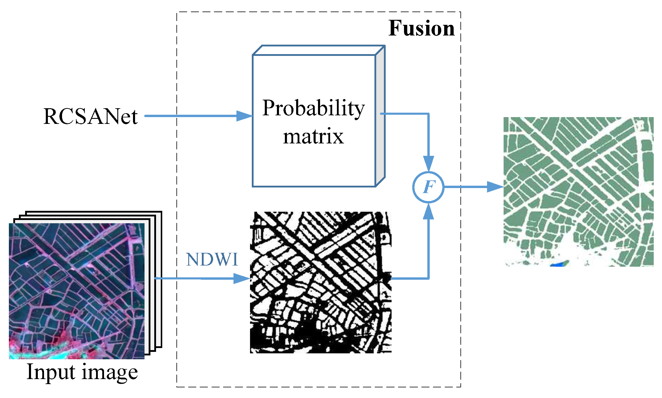
To further improve the segmentation quality of aquaculture ponds, the normalized difference water index (NDWI) maps from pansharpening images are fused with the prediction probability matrices from the proposed network to produce the final classification result (Figure 6). This implementation is called “RCSANet-NDWI”. The classification probability matrices are produced from the three classes (aquaculture ponds, natural water surfaces, and background) probability maps after the Softmax layer. Both aquaculture ponds and natural water surfaces are water bodies surrounding inland lakes. Hence, the water extraction index, which is a typical representation of the spectral characteristics of a water body used to distinguish ground features, has been extensively used. The NDWI maps were used to provide prior knowledge for aquaculture pond extraction. Through OTSU threshold binary segmentation [43], NDWI maps were divided into water and non-water parts. The water parts in the NDWI maps were used to refine the three-class probability matrix described earlier. Assume that the original probability matrix P 0 and the refined matrix P are both h × w × c in size, whereas the NDWI map S is h × w in size. c is the channel number, k is the channel ID, and the kth channel represents the kth class. Hence, k = 1 , 2 , 3 represent background, water, and aquaculture ponds, respectively. The fusion operation can be defined as:
P i j k = P 0 i j k , k 1 y i j · P 0 i j k , k = 1
where y is the indicator variable
y i j = 0 , S i j = 1 1 , S i j = 0
For the pixel in the i-th row and j-th column of S, if its value is 1 (representing water), the corresponding background probability ( k = 1 ) in P 0 is set to 0, and the fused matrix P is generated. The final classification maps can be obtained using the maximum probability judgment. The maximum probability judgment is the usual method for mapping the probability matrix to the final label image: the classification label of this pixel is determined with maximum probability: l i j = arg max k ( p i j k ) , where probability p i j k is the probability of a pixel in the i-th row and j-th column from k different sources. With the NDWI, the interference from the background of the water body extraction is eliminated because the probability of the non-water part is set to 0.

4. Experiments

This section describes a series of qualitative and quantitative comprehensive evaluations that were conducted using the proposed methods with the dataset introduced in Section 2.

4.1. Experimental Set-Up

The inputs of the proposed network were 256 × 256 pansharpening patches with three spectral channels. Table 2 lists the parameters of the convolution kernels, which are basic operators of different modules in the entire process of the proposed RCSANet. Parameter rate means that the convolution kernels in different atrous convolution branches of the ASPP-RC module have different padding and dilation configurations, which are set to 6, 12, and 18, respectively, according to Figure 3b. Validation consisted of two parts:
(1)
Evaluating the performance of the proposed methods. The pansharpening images of the six regions (both type I and type II in Figure 1) were segmented into image patches 256 × 256 pixels in size. These image slices were randomly divided into training and test sets, of which 80% (4488 images) made up the training set and 20% (1122 images) made up the test set. The overall accuracy, user’s accuracy, producer’s accuracy, and kappa coefficients were used as the main evoluation metrics.
(2)
To assess the quality of aquaculture pond extraction and evaluate the generalization and migration capabilities of RCSANet, four regions (type I) were used as training data, and the other two regions (type II) were used as test areas. The overall accuracy, user’s accuracy, producer’s accuracy, and kappa coefficients were calculated to assess aquaculture pond extraction accuracy on the 2 m spatial resolution pansharpened images.
In addition, the proposed methods were divided into two versions: RCSANet (without NDWI fusion) and RCSANet-NDWI (with NDWI fusion) to verify the role of NDWI fusion. Three state-of-the-art segmentation methods, including DeeplabV3+ [20], Reseg [44], and Homogeneous Convolutional Neural Network (HCN) [25] were selected for comparison. In addition, the performance of SVM was also assessed as a representative of traditional machine learning methods that directly use each pixel as a feature. DeeplabV3+ is an FCN method for semantic segmentation with the help of an ASPP module. Reseg is a hybrid deep network for semantic segmentation. Except for CNN, the bidirectional GRU is also used in Reseg to capture contextual dependencies. HCN was originally proposed for automatic raft labelling and is now considered to have potential for aquaculture pond extraction. HCN was implemented following the settings in [25], and Resnet-101 was simultaneously used as the encoder in DeeplabV3+, Reseg, and the proposed methods.
In the present experiments, the parameters of the proposed methods were optimized by minibatch stochastic gradient descent using a momentum algorithm with a batch size of 2. The learning rate was set to 10 2 and decayed with training epoch according to the “polynomial” strategy. The number of training epochs was configured as 40. The SVM was implemented with the help of the LIBSVM package [45], and two important factors, C and γ , were determined through a five-fold cross validation grid search. Except for the HCN, which was operated using TensorFlow 1.9.0, the other deep learning-based algorithms were implemented in Pytorch 1.1.0. All deep learning methods were implemented on a single NVIDIA GeForce GTX 1080 GPU.

4.2. Results

The performance of the various semantic segmentation methods in Part 1 of the experiments is depicted in Table 3. Clearly, the deep learning-based methods perform better than the traditional SVM algorithm because the latter cannot perceive spatial semantic information in the image. DeeplabV3+ is a state-of-the-art FCN method that has been widely used. Resnet-101 was also chosen as the backbone for DeeplabV3+. HCN is a deep convolutional neural network for automatic raft labelling, and Reseg is a deep recurrent neural network for semantic segmentation. The classification accuracy of the proposed methods for natural water surfaces and aquaculture ponds was consistently better than the other methods. Meanwhile, compared with DeeplabV3+, the overall accuracy in the two versions of the proposed methods led to an improvement of more than 7% and the Kappa coefficients of the proposed methods were greater than 0.72, indicating that the proposed method is significantly better than DeeplabV3+. Moreover, the results also demonstrated the effect of the proposed fusion strategy because RCSANet-NDWI further surpassed RCSANet on most metrics.
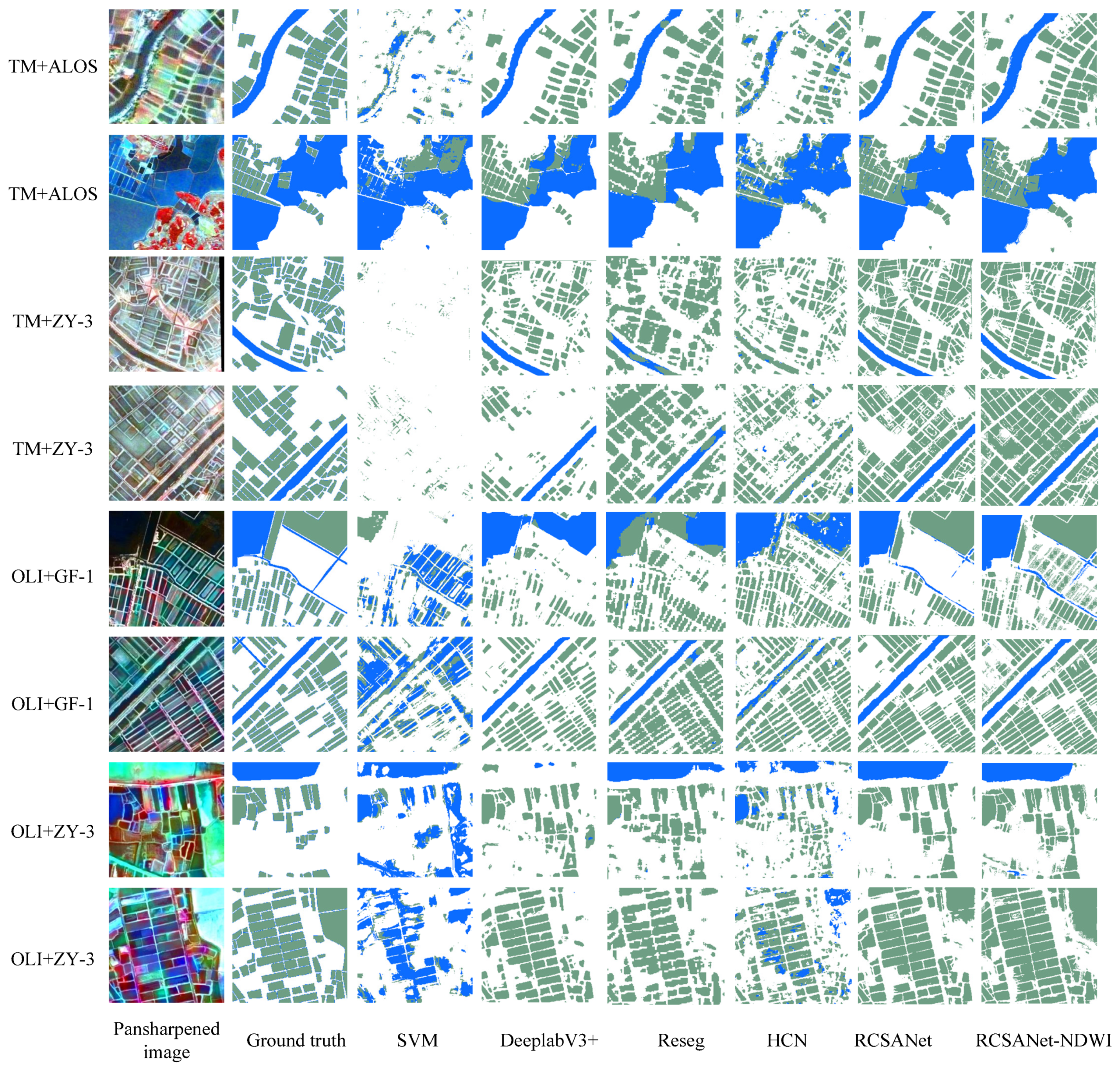
Figure 7 gives a detailed display of the classification results in Part 1 of the experiment. Inland water areas contain various natural water bodies as well as aquaculture ponds. These natural water bodies greatly interfere with the segmentation result for aquaculture ponds, making pixel-scale classification intricate. Figure 7 shows that the SVM classification results misclassified many aquaculture ponds as natural water bodies and many natural water bodies as aquaculture ponds, indicating that the traditional pixel-based method cannot efficiently distinguish natural water bodies from aquaculture ponds. The segmentation maps created by DeeplabV3+ look significantly better than those from SVM, but in some difficult zones where natural water bodies look similar to aquaculture ponds, they are also trapped by their own performance limitations and misclassified natural water bodies as aquaculture ponds (area in the 7th row) or aquaculture ponds as natural water bodies (districts in the 5th row). HCN, which has good performance for raft-culture extraction in offshore waters, performed poorly on semantic segmentation of inland aquaculture ponds and serious misclassifications also happened with HCN. Reseg, which combines CNN and bidirectional GRU, can perform semantic segmentation for aquaculture ponds. However, the identification of natural water bodies that closely resemble aquaculture ponds around inland lakes is not as good as with the proposed methods. In Table 3, the overall accuracy of the Reseg method can reach greater than 80% but its Kappa coefficient is less than 0.7. This shows that Reseg has established a spatial relationship through the construction of GRU, which has a certain effect on the segmentation of aquaculture ponds around inland lakes, but it is not good enough. In the Reseg segmentation map, many objects are stuck together, and the edges of aquaculture ponds are not well displayed. Among these result maps, the two versions of the proposed method separated natural water bodies and aquaculture ponds more satisfactorily than the other methods. The ASPP-RC module of the proposed method feeds back the details at different scales into the low-level feature map, which can draw visual attention to the decoding part. This facilitates identification of the thin edges surrounding the aquaculture ponds in semantic segmentation. Hence, the edges of aquaculture ponds were clearly identified in most cases, as shown in the results from RCSANet and RCSANet-NDWI. Finally, note that RCSANet-NDWI further improved the quality of aquaculture pond extraction compared with RCSANet.
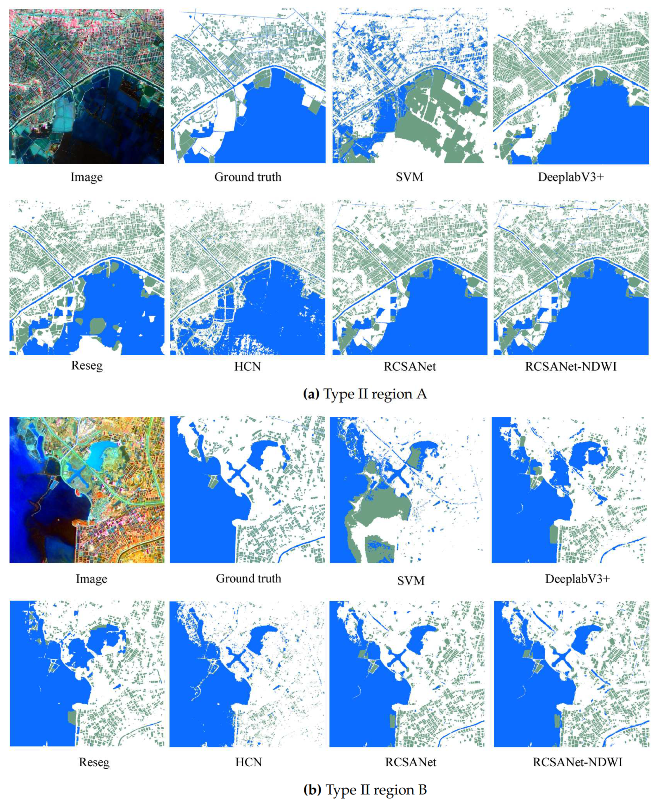
Table 4 provides assessment results for the various algorithms in Part 2 of the experiment and shows the corresponding extraction accuracies of the aquaculture pond and natural water surface classes in the two experimental areas (regions A and B in Figure 1) by different sensors. The overall accuracy and Kappa coefficient show that the two versions of the proposed method (RCSANet and RCSANet-NDWI) both performed better than the other methods, regardless of sensor or area. Moreover, compared with RCSANet, the accuracy of RCSANet-NDWI was further improved with the aid of NDWI fusion. In region A, their overall accuracies in pansharpening images from different sensors were greater than 85 percent, and the Kappa coefficients were definitely greater than 0.7. These results were better than those of other deep learning-based methods, not to mention SVM. In region B, the proposed methods still performed the best. Unlike region A, where the lake is greatly influenced by residents living nearby, causing the aquaculture ponds to be neatly and regularly distributed, the aquaculture ponds in region B have a sparser distribution. Region B is relatively well protected, and some small natural water bodies, which are easily confused with aquaculture ponds and interfere with network identification, were produced when the lake was split for artificial development. Hence, the situations in the two regions are completely different, which shows the stability of the proposed methods under various scenarios. The overall accuracies of the proposed methods in pansharpening images from different regions were close to or greater than 80 percent. In addition, it should be noted that user accuracy in identifying natural water bodies in almost all methods is relatively high. This is because natural water bodies tend to be extensive, homogeneous, self-contained, and distributed in aggregates, a situation that is easier to recognize for the classifier. Compared with the proposed methods, Reseg and DeeplabV3+ may also obtain higher user accuracy in some cases. However, because of their limited recognition ability, they cannot explicitly judge the difference between aquaculture ponds and natural water bodies (Figure 8).
Figure 8 shows the classification results in the two study regions. Extracting aquaculture ponds in region B is more difficult than in region A because region B contains more natural water bodies that are hard to distinguish from aquaculture ponds. The two versions of the proposed method performed significantly better than the other methods for aquaculture pond extraction. The proposed methods were predominantly successful in predicting aquaculture ponds that are divided into regular shapes by embankments, as well as the natural water bodies in the two regions. In region A, the proposed methods generally extracted almost all aquaculture ponds compared with the ground truth, whereas other methods failed, especially in the upper part of the scene. In region B, compared with Reseg, the proposed methods had lower misclassification rates, and the natural rivers located at the bottom, which could not be identified by Reseg, were not misclassified as aquaculture ponds by the proposed methods. Moreover, the shapes of the ponds are best retained, as shown in the results of the proposed method. The advantage of the proposed method is the proposed RCSA mechanism for determining salient pixels in a row or column, which is essentially a description of the pixel-level context. This enables the proposed method to identify detailed features of the 2 m spatial resolution image, where the dikes around aquaculture ponds are such pixel-level details. Hence, the aquaculture ponds in region B were more fully extracted by the proposed RCSANet than by other state-of-the-art methods, such as DeeplabV3+ and Reseg. On the other hand, fusion using NDWI can better distinguish water surfaces, including natural water bodies and aquaculture ponds, from background. In effect, the proposed method with NDWI re-segments the leaked water surface from the background, which improves the producer’s accuracy of the aquaculture pond. However, this also entails a phenomenon whereby a small part of the background is mistakenly classified as water surface.

5. Discussion

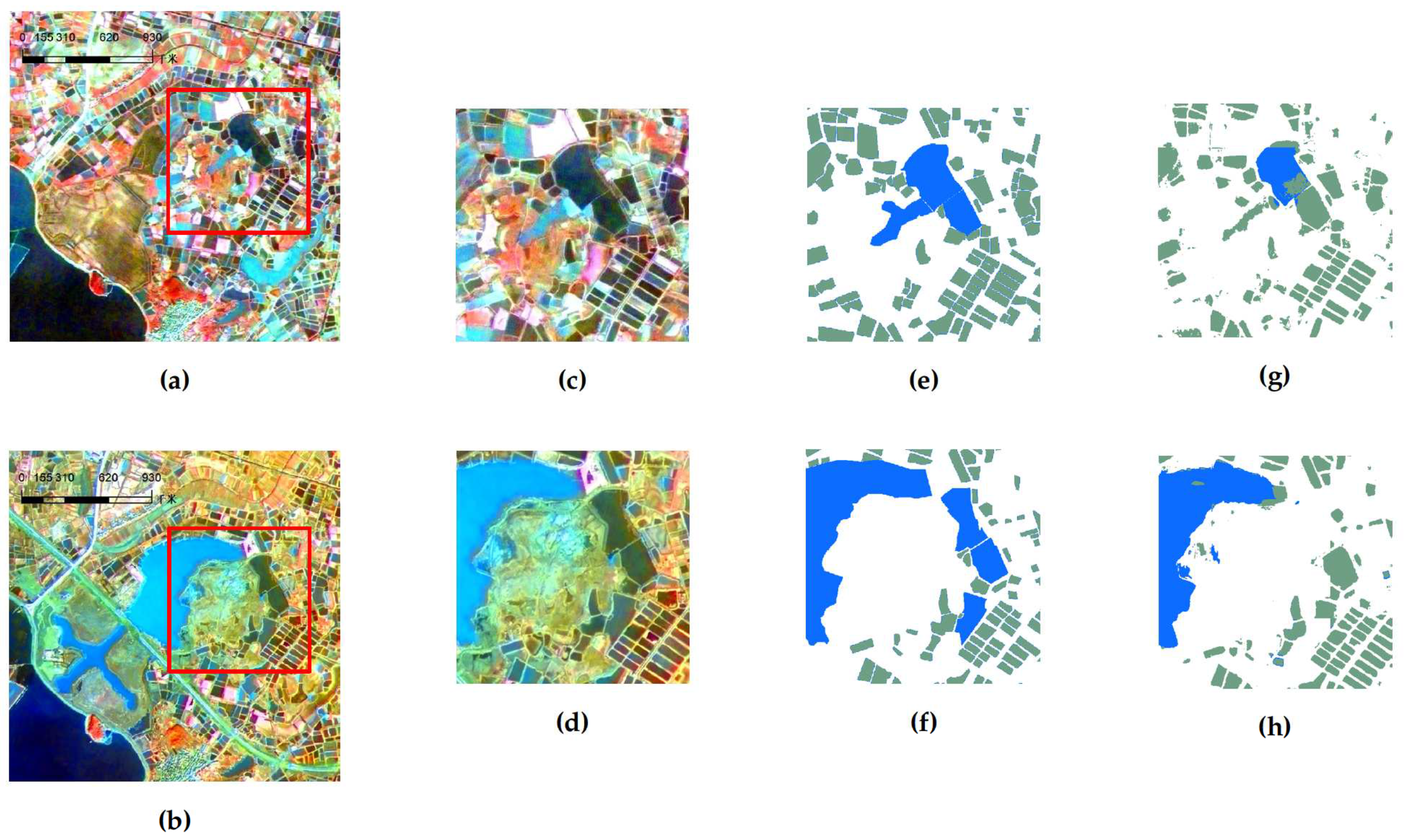
This study has used a fully convolutional network architecture with row- and column-wise self-attention to semantically segment aquaculture ponds around inland lakes. Artificial aquaculture ponds around inland lakes are small, and the dikes between these ponds are only about 2 m wide. On medium-resolution multispectral images, water pixels are firstly separated from land, and then water objects are formed based on connectivity. After that, these water objects are classified as natural water bodies and aquaculture ponds using geometric characteristics [8]. However, for inland lake area where aquaculture ponds are intensively distributed with narrow dikes (e.g., Lake Hong), the 15–30 m spatial resolution of the image limits the capability of the object based method to accurately extract aquaculture ponds. Hence, finer-spatial-resolution images are considered for pond extraction. By fusing multi-spectral information into panchromatic images from the GF-1, ZY-3 or ALOS satellites, the spatial resolution of the resultant satellite images can achieve up to 2 meters, enabling the identification of thin narrow dams. Meanwhile, the multi-spectral capability is utilized to recognize water. From the segmentation results, the proposed network structure was shown to be capable of extracting these regular pond boundaries, mainly because semantic segmentation of the aquaculture ponds benefits from establishing a spatial relationship between pixels in the same direction by the self-attention model. Although HCN was also an FCN-based method used to automatic raft labeling [25], nevertheless, its performance for extracting aquaculture ponds around inland lakes are not as effective as that for labeling raft-culture. Because the spatial context of raft-culture in coastal area is much simple than that of the inland lake area. In general, through high-spatial-resolution images that incorporate multi-spectral and panchromatic data, the proposed RCSANet enables the extraction of large-scale aquaculture ponds around inland lakes where complex spatial contexts of water surfaces exist. However, it is still challenging for the recognition of small water bodies in such complex spatial context. The experimental region B was in the process of recovering aquaculture ponds and farmland as lake area from 2011 to 2014. Therefore, various aquaculture ponds and natural water bodies are spatially mixed on the images of pansharpening multispectral and panchromatic data from 2011 and 2014, which poses great challenges for semantic segmentation of aquaculture ponds. For example, Figure 9c,d are images of the same area, which changed significantly between 2011 and 2014. Several small reservoirs were apparent in Figure 9c, but the profiles of these reservoirs had changed significantly in Figure 9d, and the left side of this area had been recovered into a large lake. The segmentation results in Figure 9g,f show that the restored large lake has been well segmented, but the small reservoirs are easily classified as aquaculture ponds or missed segmentations.
In the paper, extracting aquaculture ponds is performed on images that pansharpen multi-spectral data from Landsat satellites and panchromatic data from other satellites in the same period, and therefore the semantic segmentation might also be affected by the spectral range of the panchromatic image. Table 5 gives the results of an accuracy analysis that divided the training data of Part 2 of the experiment into two portions: pansharpened TM images and pansharpened OLI images. The predicted results of pansharpened TM images from Region B are based on RSCANet, which was trained by fusing TM images with panchromatic images from ZY-3 or ALOS satellites. The predicting results of pansharpened OLI images from Region B is based on RSCANet, which was trained by fusing OLI images with panchromatic images from GF-1 satellites. Table 5 shows that the results of pansharpened OLI images with panchromatic images from GF-1 satellites are significantly better than the results of pansharpened TM images with panchromatic images from ZY-3 or ALOS satellites. The spectrum of panchromatic images from GF-1 satellites ranges from 0.45 to 0.90 μm, which can completely cover the three NIR, red, and green bands of Landsat OLI data. However, the spectrum of panchromatic images from ZY-3 or ALOS satellites can only partly cover the NIR band of the TM sensor. The acquisition time of the TM images was earlier than 2012, and therefore it is difficult to use a GF-1 panchromatic image for pansharpened TM images.
The RCSANet can extract aquaculture ponds around inland lakes on 2 m satellite images more accurately than other methods because the involvement of two connection groups from the encoder to the decoder. The first connection group is the combination of the RCSA module and the ASPP-RC module, which links Conv1 of encoder part to decoder part. The second is the RCSA modules, linking Res-1, Res-2, and Res-3 of encoder part to decoder part. Table 6 indicates that the first connection group of RCSANet achieves an additional 2.32% overall accuracy gains over RCSANet1, and the second connection group brings 3.59% overall accuracy gains over RCSANet2, i.e., a plain FCN architecture based on ResNet-101 model. Nevertheless, the connections expend more computing resources because they involve the non-local self-attention mechanism, which contains many inner-product operations. Moreover, the RCSANet is an encoder-decoder architecture in which the gradual upsampling are conducted, requiring more memory and calculation time. Table 7 shows that the RCSANet consumes more memory and training and prediction time than Deeplabv3+ and Reseg methods. It is feasible to sacrifice some computing resources to achieve higher accuracy of aquaculture pond extraction, especially the GPU performance will increase gradually.

6. Conclusions

This study has implemented a semantic segmentation network on high-spatial-resolution satellite images for aquaculture pond extraction. A row- and column-wise self-attention (RCSA) mechanism has been proposed to capture the intertwining regular embankments of aquaculture ponds in feature maps, and then a fully convolutional network framework combined with the RCSA mechanism is proposed for semantic segmentation of aquaculture ponds. The proposed methods have been evaluated on high-spatial-resolution pansharpened images obtained by fusing multi-spectral and panchromatic images in typical regions with inland lakes and densely distributed aquaculture ponds. Experiments on satellite images of both a highly developed lake and a reserved lake show that the overall accuracy of the proposed method is significantly better than those of other methods (3–8% overall accuracy gains at Lake Liangzi and 1–2% overall accuracy gains at Lake Hong over the best of other methods). Specifically, from the experimental semantic segmentation results for large regions, detailed information, such as the embankments of aquaculture ponds, can be more accurately identified by the proposed method. It can be concluded that the proposed method is effective for large-scale extraction of aquaculture ponds. In addition, RCSANet-NDWI further improves the accuracy of the proposed method compared with RCSANet, indicating the significance of the proposed NDWI fusion strategy. For future study, the proposed methods can be extended to raft-culture extraction in offshore waters.

Author Contributions

Conceptualization, Z.Z., W.T. and G.Y.; methodology, Z.Z. and D.W.; software, D.W. and J.Y.; validation, D.W., J.Y., B.L. and Z.W.; investigation, Z.Z., W.T. and G.Y.; writing—original draft preparation, Z.Z.; writing—review and editing, W.T., D.W. and G.Y.; visualization, D.W. and J.Y. All authors have read and agreed to the published version of the manuscript.

Funding

This work was supported partially by the National Key Research and Development Program of China under Grant 2017YFC1405600, partially by the Fundamental Research Funds for the Central Universities under Grant 18CX02060A and CCNU19TD002, and partially by the National Natural Science Foundation of China under grant 41506208.

Institutional Review Board Statement

Not applicable.

Informed Consent Statement

Not applicable.

Data Availability Statement

The data presented in this study are available on request from the corresponding author.

Acknowledgments

We are particularly grateful for help in the field and with high-resolution imagery from Jianhua Huang, National & Local Joint Engineering Research Center of Satellite Navigation and Location Service, Guilin University of Electronic Technology. We would like to acknowledge the invaluable input and assistance from the rest of the College of Oceanography and Space Informatics, China University of Petroleum, including Xuxu Kong, Weipeng Lu, Yachao Chen and Sai Zhang.

Conflicts of Interest

The authors declare no conflict of interest.

References

  1. Cao, L.; Naylor, R.; Henriksson, P.; Leadbitter, D.; Metian, M.; Troell, M.; Zhang, W. China’s aquaculture and the world’s wild fisheries. Science 2015, 347, 133–135. [Google Scholar] [CrossRef] [PubMed]
  2. Cai, C.; Gu, X.; Ye, Y.; Yang, C.; Dai, X.; Chen, D.; Yang, C. Assessment of pollutant loads discharged from aquaculture ponds around Taihu Lake, China. Aquac. Res. 2013, 44, 795–806. [Google Scholar] [CrossRef]
  3. Luo, J.; Pu, R.; Ma, R.; Wang, X.; Lai, X.; Mao, Z.; Zhang, L.; Peng, Z.; Sun, Z. Mapping long-term spatiotemporal dynamics of pen aquaculture in a shallow lake: Less aquaculture coming along better water quality. Remote Sens. 2020, 12, 1866. [Google Scholar] [CrossRef]
  4. Zhang, H.; Kang, M.; Shen, L.; Wu, J.; Li, J.; Du, H.; Wang, C.; Yang, H.; Zhou, Q.; Liu, Z.; et al. Rapid change in Yangtze fisheries and its implications for global freshwater ecosystem management. Fish Fish. 2020, 21, 601–620. [Google Scholar] [CrossRef]
  5. Ottinger, M.; Clauss, K.; Kuenzer, C. Large-scale assessment of coastal aquaculture ponds with Sentinel-1 time series data. Remote Sens. 2017, 9, 440. [Google Scholar] [CrossRef] [Green Version]
  6. Ren, C.; Wang, Z.; Zhang, Y.; Zhang, B.; Chen, L.; Xi, Y.; Xiao, X.; Doughty, R.B.; Liu, M.; Jia, M.; et al. Rapid expansion of coastal aquaculture ponds in China from Landsat observations during 1984–2016. Int. J. Appl. Earth Obs. Geoinf. 2019, 82, 101902. [Google Scholar] [CrossRef]
  7. Stiller, D.; Ottinger, M.; Leinenkugel, P. Spatio-temporal patterns of coastal aquaculture derived from Sentinel-1 time series data and the full Landsat archive. Remote Sens. 2019, 11, 1707. [Google Scholar] [CrossRef] [Green Version]
  8. Zeng, Z.; Wang, D.; Tan, W.; Huang, J. Extracting aquaculture ponds from natural water surfaces around inland lakes on medium resolution multispectral images. Int. J. Appl. Earth Obs. Geoinf. 2019, 80, 13–25. [Google Scholar] [CrossRef]
  9. Zhang, T.; Li, Q.; Yang, X.; Zhou, C.; Su, F. Automatic mapping aquaculture in coastal zone from TM imagery with OBIA approach. In Proceedings of the 2010 18th International Conference on Geoinformatics, Geoinformatics 2010, Beijing, China, 18–20 June 2010. [Google Scholar] [CrossRef]
  10. Tran, H.; Tran, T.; Kervyn, M. Dynamics of land cover/land use changes in the Mekong Delta, 1973–2011: A Remote sensing analysis of the Tran Van Thoi District, Ca Mau Province, Vietnam. Remote Sens. 2015, 7, 2899–2925. [Google Scholar] [CrossRef] [Green Version]
  11. Prasad, K.A.; Ottinger, M.; Wei, C.; Leinenkugel, P. Assessment of coastal aquaculture for India from Sentinel-1 SAR time series. Remote Sens. 2019, 11, 357. [Google Scholar] [CrossRef] [Green Version]
  12. Geng, Q.; Zhou, Z.; Cao, X. Survey of recent progress in semantic image segmentation with CNNs. Sci. China Inf. Sci. 2018, 61, 051101. [Google Scholar] [CrossRef] [Green Version]
  13. Lecun, Y.; Bengio, Y.; Hinton, G. Deep learning. Nature 2015, 521, 436–444. [Google Scholar] [CrossRef] [PubMed]
  14. Simonyan, K.; Zisserman, A. Very Deep Convolutional Networks for Large-Scale Image Recognition. In Proceedings of the International Conference on Learning Representations, San Diego, CA, USA, 7–9 May 2015. [Google Scholar]
  15. He, K.; Zhang, X.; Ren, S.; Sun, J. Deep residual learning for image recognition. In Proceedings of the IEEE Computer Society Conference on Computer Vision and Pattern Recognition, Las Vegas, NV, USA, 27–30 June 2016; pp. 770–778. [Google Scholar] [CrossRef] [Green Version]
  16. Shelhamer, E.; Long, J.; Darrell, T. Fully Convolutional Networks for Semantic Segmentation. IEEE Trans. Pattern Anal. Mach. Intell. 2017, 39, 640–651. [Google Scholar] [CrossRef] [PubMed]
  17. Badrinarayanan, V.; Kendall, A.; Cipolla, R. SegNet: A Deep Convolutional Encoder-Decoder Architecture for Image Segmentation. IEEE Trans. Pattern Anal. Mach. Intell. 2017, 39, 2481–2495. [Google Scholar] [CrossRef] [PubMed]
  18. Chen, L.C.; Papandreou, G.; Kokkinos, I.; Murphy, K.; Yuille, A.L. DeepLab: Semantic Image Segmentation with Deep Convolutional Nets, Atrous Convolution, and Fully Connected CRFs. IEEE Trans. Pattern Anal. Mach. Intell. 2018, 40, 834–848. [Google Scholar] [CrossRef] [PubMed]
  19. Chen, L.; Papandreou, G.; Schroff, F.; Adam, H. Rethinking Atrous Convolution for Semantic Image Segmentation. arXiv 2017, arXiv:1706.05587. [Google Scholar]
  20. Chen, L.; Zhu, Y.; Papandreou, G.; Schroff, F.; Adam, H. Encoder-Decoder with Atrous Separable Convolution for Semantic Image Segmentation. arXiv 2018, arXiv:1802.02611. [Google Scholar]
  21. Lateef, F.; Ruichek, Y. Survey on semantic segmentation using deep learning techniques. Neurocomputing 2019, 338, 321–348. [Google Scholar] [CrossRef]
  22. Du, P.; Bai, X.; Tan, K.; Xue, Z.; Samat, A.; Xia, J.; Li, E.; Su, H.; Liu, W. Advances of Four Machine Learning Methods for Spatial Data Handling: A Review. J. Geovisualization Spat. Anal. 2020, 4, 13. [Google Scholar] [CrossRef]
  23. Audebert, N.; Le Saux, B.; Lefèvre, S. Beyond RGB: Very high resolution urban remote sensing with multimodal deep networks. ISPRS J. Photogramm. Remote Sens. 2018, 140, 20–32. [Google Scholar] [CrossRef] [Green Version]
  24. Wurm, M.; Stark, T.; Zhu, X.X.; Weigand, M.; Taubenböck, H. Semantic segmentation of slums in satellite images using transfer learning on fully convolutional neural networks. ISPRS J. Photogramm. Remote Sens. 2019, 150, 59–69. [Google Scholar] [CrossRef]
  25. Shi, T.; Xu, Q.; Zou, Z.; Shi, Z. Automatic Raft Labeling for Remote Sensing Images via Dual-Scale Homogeneous Convolutional Neural Network. Remote Sens. 2018, 10, 1130. [Google Scholar] [CrossRef] [Green Version]
  26. Cui, B.; Fei, D.; Shao, G.; Lu, Y.; Chu, J. Extracting raft aquaculture areas from remote sensing images via an improved U-net with a PSE structure. Remote Sens. 2019, 11, 2053. [Google Scholar] [CrossRef] [Green Version]
  27. Mnih, V.; Heess, N.; Graves, A.; Kavukcuoglu, K. Recurrent Models of Visual Attention. Adv Neural Inf Process Syst. 2014, 2, 2204–2212. [Google Scholar]
  28. Bahdanau, D.; Cho, K.; Bengio, Y. Neural Machine Translation by Jointly Learning to Align and Translate. arXiv 2015, arXiv:1409.0473. [Google Scholar]
  29. Luong, T.; Pham, H.; Manning, C.D. Effective Approaches to Attention-based Neural Machine Translation. In Proceedings of the 2015 Conference on Empirical Methods in Natural Language Processing, Lisbon, Portugal, 17–21 September 2015; pp. 1412–1421. [Google Scholar] [CrossRef] [Green Version]
  30. Xu, K.; Ba, J.L.; Kiros, R.; Cho, K.; Courville, A.; Salakhutdinov, R.; Zemel, R.S.; Bengio, Y. Show, attend and tell: Neural image caption generation with visual attention. In Proceedings of the 32nd International Conference on Machine Learning, ICML 2015, Lille, France, 6–11 July 2015; Volume 3, pp. 2048–2057. [Google Scholar]
  31. Parmar, N.; Vaswani, A.; Uszkoreit, J.; Kaiser, Ł.; Shazeer, N.; Ku, A.; Tran, D. Image Transformer. In Proceedings of the 35th International Conference on Machine Learning, Stockholmsmässan, Stockholm, Sweden, 10–15 July 2018. [Google Scholar]
  32. Vaswani, A.; Shazeer, N.; Parmar, N.; Uszkoreit, J.; Jones, L.; Gomez, A.N.; Kaiser, L.; Polosukhin, I. Attention Is All You Need. In Proceedings of the 31st Conference on Neural Information Processing Systems (NIPS 2017), Long Beach, CA, USA, 4–9 December 2017. [Google Scholar]
  33. Fu, J.; Liu, J.; Tian, H.; Li, Y.; Bao, Y.; Fang, Z.; Lu, H. Dual Attention Network for Scene Segmentation. arXiv 2019, arXiv:1809.02983. [Google Scholar]
  34. Xu, X.; Huang, X.; Zhang, Y.; Yu, D.; Xu, X.; Huang, X.; Zhang, Y.; Yu, D. Long-Term Changes in Water Clarity in Lake Liangzi Determined by Remote Sensing. Remote Sens. 2018, 10, 1441. [Google Scholar] [CrossRef] [Green Version]
  35. Hua, Y.; Mou, L.; Zhu, X.X. Recurrently exploring class-wise attention in a hybrid convolutional and bidirectional LSTM network for multi-label aerial image classification. ISPRS J. Photogramm. Remote Sens. 2019, 149, 188–199. [Google Scholar] [CrossRef]
  36. Gao, H.; Gu, X.; Yu, T.; Liu, L.; Sun, Y.; Xie, Y.; Liu, Q. Validation of the calibration coefficient of the GaoFen-1 PMS sensor using the landsat 8 OLI. Remote Sens. 2016, 8, 132. [Google Scholar] [CrossRef] [Green Version]
  37. Jiang, Y.H.; Zhang, G.; Tang, X.M.; Li, D.; Huang, W.C.; Pan, H.B. Geometric calibration and accuracy assessment of ZiYuan-3 multispectral images. IEEE Trans. Geosci. Remote Sens. 2014, 52, 4161–4172. [Google Scholar] [CrossRef]
  38. Maurer, T. How to pan-sharpen images using the Gram-Schmidt pan-sharpen method—A recipe. In Proceedings of the ISPRS Hannover Workshop 2013, Hannover, Germany, 21–24 May 2013; Volume XL-1/W1, pp. 239–244. [Google Scholar] [CrossRef] [Green Version]
  39. Sekrecka, A.; Kedzierski, M.; Wierzbicki, D. Pre-processing of panchromatic images to improve object detection in pansharpened images. Sensors 2019, 19, 5146. [Google Scholar] [CrossRef] [PubMed] [Green Version]
  40. Yu, C.; Wang, J.; Peng, C.; Gao, C.; Yu, G.; Sang, N. Learning a Discriminative Feature Network for Semantic Segmentation. In Proceedings of the IEEE Computer Society Conference on Computer Vision and Pattern Recognition, Salt Lake City, UT, USA, 18–22 June 2018; Volume 1, pp. 1857–1866. [Google Scholar] [CrossRef] [Green Version]
  41. Zhao, R.; Wang, D.; Yan, R.; Mao, K.; Shen, F.; Wang, J. Machine Health Monitoring Using Local Feature-Based Gated Recurrent Unit Networks. IEEE Trans. Ind. Electron. 2018, 65, 1539–1548. [Google Scholar] [CrossRef]
  42. Galassi, A.; Lippi, M.; Torroni, P. Attention in Natural Language Processing. arXiv 2020, arXiv:1902.02181. [Google Scholar] [CrossRef] [PubMed]
  43. Otsu, N. A Threshold Selection Method from Gray-Level Histograms. IEEE Trans. Syst. Man Cybern. 1979, 9, 62–66. [Google Scholar] [CrossRef] [Green Version]
  44. Visin, F.; Romero, A.; Cho, K.; Matteucci, M.; Ciccone, M.; Kastner, K.; Bengio, Y.; Courville, A. ReSeg: A Recurrent Neural Network-Based Model for Semantic Segmentation. In Proceedings of the 2016 IEEE Conference on Computer Vision and Pattern Recognition Workshops (CVPRW), Las Vegas, NV, USA, 28 June–1 July 2016; pp. 426–433. [Google Scholar] [CrossRef] [Green Version]
  45. Chang, C.C.; Lin, C.J. LIBSVM: A Library for Support Vector Machines. ACM Trans. Intell. Syst. Technol. TIST 2013, 2, 1–39. [Google Scholar] [CrossRef]
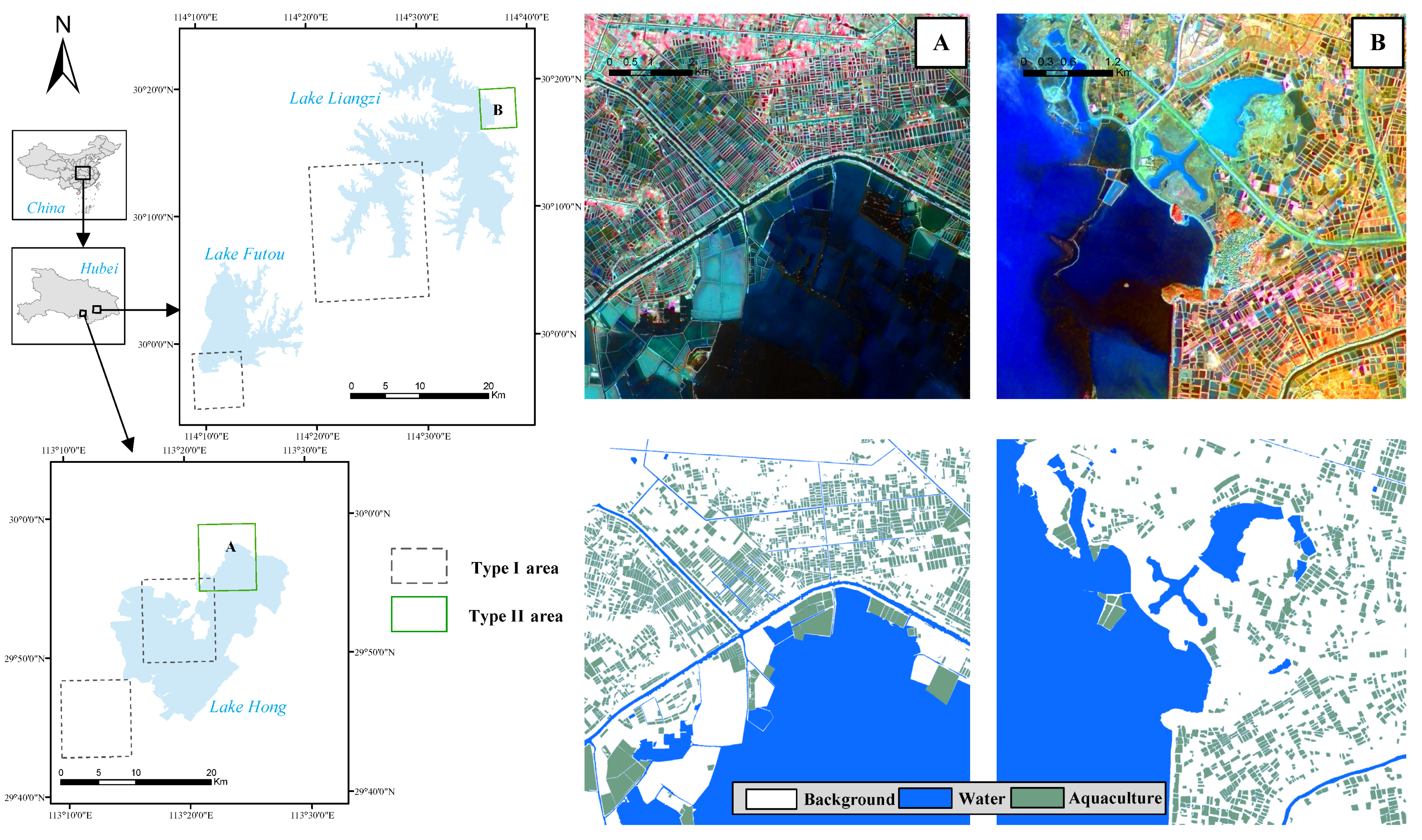
Figure 1. Location of the study area. The pseudo-colour images (A,B) are pansharpening images using the near infrared, the red and the green band as red, green and blue. The corresponding labelling image for each is given below.
Remotesensing 13 00092 g001
Figure 2. Field photos of inland aquaculture ponds in Hubei Province, China. Aquaculture ponds are usually equipped with air pumps. (A) A branch of a natural lake. (B) An aquaculture pond equipped with oxygen pumps. (C) Below is a small river (natural water body) and above are several aquaculture ponds.
Remotesensing 13 00092 g002
Figure 3. RCSANet: FCN architecture combined with RCSA mechanism for semantic segmentation of aquaculture ponds: (a) Network architecture; (b) ASPP-RC module; (c) Upsampling block. The input image of the entire deep neural network is a 256 × 256 pansharpening patch with three spectral channels. Through encoding and decoding, a three-channel matrix for classification was output through a 1 × 1 convolution layer at the end, and finally a Softmax layer gave a prediction map with the same size as the input image.
Remotesensing 13 00092 g003
Figure 4. Attention models.
Remotesensing 13 00092 g004
Figure 5. Attention layer consisting of column-wise and row-wise self-attention models.
Remotesensing 13 00092 g005
Figure 6. Fusion strategy.
Remotesensing 13 00092 g006
Figure 7. Semantic segmentation results for 256 × 256 pixel image patches from test set in Part 1 of the experiment. The leftmost column gives the sensors or satellites to which the multispectral and panchromatic data of the pansharpened images belong, and the bottom row lists the different methods by which the semantic segmentation images in the same column were obtained.
Remotesensing 13 00092 g007
Figure 8. Semantic segmentation results for aquaculture ponds and natural water bodies by various methods: (a) in region A, using the pansharpened image with the TM multispectral image captured in January 2011 and the ZY-3 panchromatic image in January 2013; and (b) in region B, using the pansharpened image with the OLI multispectral image captured in February 2014 and the GF-1 panchromatic image in January 2014.
Remotesensing 13 00092 g008
Figure 9. Influence of multi-year changes on semantic segmentation results for aquaculture ponds. (a,b) are pansharpened images of the significantly changed area from Region B in 2010 and 2014 respectively. (c,d) are magnified images. (e,f) are labelling images for (c,d). (g,h) are semantic segmentation results for (c,d) using the proposed method.
Remotesensing 13 00092 g009
Table 1. Satellite images information for various regions.
Multispectral ImagesPanchromatic Images
RegionsSensorsSpatial
Resolution (m)
DateSensorsSpatial
Resolution (m)
Date
Lake Hong (west, type I region)TM (Landsa 5)302011.01.15PAN-NAD(ZY-3)2.12013.01.27
Lake Hong (west, type I region)OLI (Landsat 8)302014.01.23PMS2(GF-1)22014.01.23
Lake Hong (middle, type I region)TM (Landsat 5)302011.01.15PAN-NAD(ZY-3)2.12013.01.27
Lake Hong (middle, type I region)OLI (Landsat 8)302014.01.23PMS2(GF-1)22014.01.23
Lake Futou (south, type I region)OLI (Landsat 8)302015.03.31PAN-NAD(ZY-3)2.12017.01.22
Lake Liangzi (west, type I region)TM (Landsat 5)302010.11.12PRISM(ALOS)2.52010.11.06
Lake Liangzi (west, type I region)OLI (Landsat 8)302014.02.01PMS2(GF-1)22014.01.31
Lake Hong (east, type II region A)TM (Landsat 5)302011.01.15PAN-NAD(ZY-3)2.12013.01.27
Lake Hong (east, type II region A)OLI (Landsat 8)302014.01.23PMS2(GF-1)22014.01.23
Lake Liangzi (east, type II region B)TM (Landsat 5)302010.11.12PRISM(ALOS)2.52010.11.06
Lake Liangzi (east, type II region B)OLI (Landsat 8)302014.02.01PMS2(GF-1)22014.01.31
Table 2. Parameters used for the convolution kernels in the various modules in RCSANet.
ModuleKernel SizeStridePaddingDilation
Conv1 × 1101
RCSA1 × 1101
Upsampling block1 × 1101
ASPP-RC(Conv)1 × 1101
ASPP-RC(Atrous conv)3 × 31raterate
Table 3. Performance comparison of different methods for semantic segmentation of aquaculture ponds in Part 1 of the experiments (%).
Producer’s AccuracyUser’s Accuracy
MethodsOverall
Accuracy (%)
KappaNatural
Water (%)
Aqua-
Culture (%)
Natural
Water (%)
Aqua-
Culture (%)
SVM26.909.7154.8015.9652.4376.60
Deeplabv3+79.1659.2390.3255.2697.9093.14
Reseg84.5268.2390.7471.1897.4490.31
HCN74.5349.8686.8348.2192.7185.74
RCSANet86.9572.8392.8374.3698.1393.99
RCSANet-NDWI89.3177.2893.2880.8198.0793.57
Table 4. Accuracy evaluation for the two classes, aquaculture ponds and natural water surfaces, in each experimental area (%).
Producer’s AccuracyUser’s Accuracy
RegionsSensorsMethodsOverall
Accuracy (%)
KappaNatural
Water (%)
Aqua-
Culture (%)
Natural
Water (%)
Aqua-
Culture (%)
Lake Hong (East,
type II region A)
TM+ZY-3SVM24.445.0927.5523.8053.8386.72
Deeplabv3+81.3060.9387.8764.7198.2583.30
Reseg84.7466.9288.9774.0697.8582.52
HCN77.3752.8588.8348.4296.7379.79
RCSANet86.7970.8390.7976.7098.2584.47
RCSANet-NDWI88.7774.7891.0882.9498.2184.42
OLI+GF-1SVM67.6025.9938.8278.7547.0982.16
Deeplabv3+84.9669.7387.6079.5796.8290.01
Reseg76.4755.1078.3072.7592.4483.38
HCN73.7648.2382.9055.0788.0286.79
RCSANet85.3669.1490.5774.7093.5990.38
RCSANet-NDWI86.6171.4391.0777.5093.6190.14
Lake Liangzi (East,
type II region B)
TM+ALOSSVM39.2614.5167.375.3286.6219.22
Deeplabv3+74.6053.4886.7350.6999.2582.83
Reseg75.2754.3384.9456.2097.8683.28
HCN67.6840.2390.0523.6092.5186.44
RCSANet79.9562.0189.3161.5099.5690.03
RCSANet-NDWI83.8568.4289.6372.4599.5189.03
OLI+GF-1SVM39.433.2948.197.5894.435.90
Deeplabv3+82.3155.9891.4549.0698.9177.99
Reseg87.9767.8493.7466.9697.8585.59
HCN77.2543.8391.8024.3197.1981.96
RCSANet90.9075.8693.0083.2699.2183.97
RCSANet-NDWI91.7177.8393.1986.3199.2083.69
Table 5. Accuracy comparation of semantic segmentation results for region B by dividing the training data of Part 2 of the experiment into pansharpened TM images and pansharpened OLI images (%).
Producer’s AccuracyUser’s Accuracy
RegionsSensorsMethodsTraining DataOverall
Accuracy (%)
KappaNatural
Water (%)
Aqua-
Culture (%)
Natural
Water (%)
Aqua-
Culture (%)
Lake Liangzi (East, type II region B)TM+ALOSRCSANetAll pansharpened images from type I regions79.9562.0189.3161.5099.5690.03
RCSANet-NDWI83.8568.4289.6372.4599.5189.03
RCSANetPansharpened images of fusing TM images with panchromatic images
from ZY-3 or ALOS satellites, from type I regions
77.4457.5490.9850.7598.7191.26
RCSANet-NDWI81.8464.6891.2363.3398.6591.00
OLI+GF-1RCSANetAll pansharpened images from type I regions90.9075.8693.0083.2699.2183.97
RCSANet-NDWI91.7177.8393.1986.3199.2083.69
RCSANetPansharpened images of fusing OLI images with panchromatic images
from GF-1 satellites, from type I regions
88.0168.7892.9270.1298.9685.70
RCSANet-NDWI89.4172.0993.1475.8598.8985.93
Table 6. Accuracy evaluation for RCSANet and its two varants RCSANet1 and RCSANet2 in Part 1 of the experiments (%). RCSANet1 is a RCSANet variant ablating the first connection group and RCSANet2 is the other variant ablating both connection groups.
MethodsOverall AccuracyKappa Coefficient
RCSANet281.0466.15
RCSANet184.6371.59
RCSANet86.9572.83
Table 7. Performance evaluation of different deep-learning based methods for semantic segmentation of aquaculture ponds in Part 2 of the experiments.
MethodsTraining Time (seconds)Occupied Memory of GPU for Training (MB)Prediction Time for Region B (seconds)Occupied Memory of GPU for Prediction (MB)
RCSA60,2807563351543
HCN66,0007709647843
Deeplabv3+16,7603113121417
Reseg10,6402343161083
Publisher’s Note: MDPI stays neutral with regard to jurisdictional claims in published maps and institutional affiliations.