Figure 1.
The difference between mountain vertex and the mountain peak. (a) A mountain with a single peak (the mountain vertex coincides with the mountain peak); (b) A mountain with two or multiple peaks (the mountain vertex is not always the same as the mountain peaks).
Figure 1.
The difference between mountain vertex and the mountain peak. (a) A mountain with a single peak (the mountain vertex coincides with the mountain peak); (b) A mountain with two or multiple peaks (the mountain vertex is not always the same as the mountain peaks).
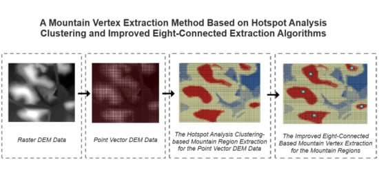
Figure 2.
The overall technical route.
Figure 2.
The overall technical route.
Figure 3.
The resample processing of the Nearest Neighbor Interpolation Algorithm.
Figure 3.
The resample processing of the Nearest Neighbor Interpolation Algorithm.
Figure 4.
Normal distribution of p-value and Z-score.
Figure 4.
Normal distribution of p-value and Z-score.
Figure 5.
The four-way optimization labeled graph of the Improved Eight-Connected Extraction Algorithm.
Figure 5.
The four-way optimization labeled graph of the Improved Eight-Connected Extraction Algorithm.
Figure 6.
The diagram of secondary Marking Method.
Figure 6.
The diagram of secondary Marking Method.
Figure 7.
Schematic diagram of mountain vertex extraction based on the Improved Eight-Connected Extraction Algorithm.
Figure 7.
Schematic diagram of mountain vertex extraction based on the Improved Eight-Connected Extraction Algorithm.
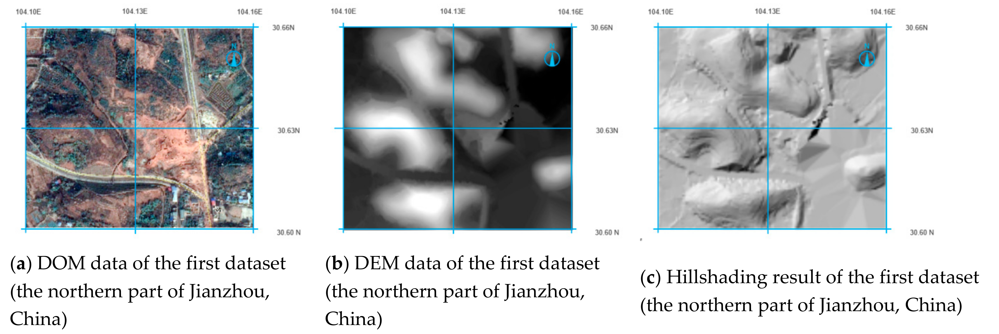
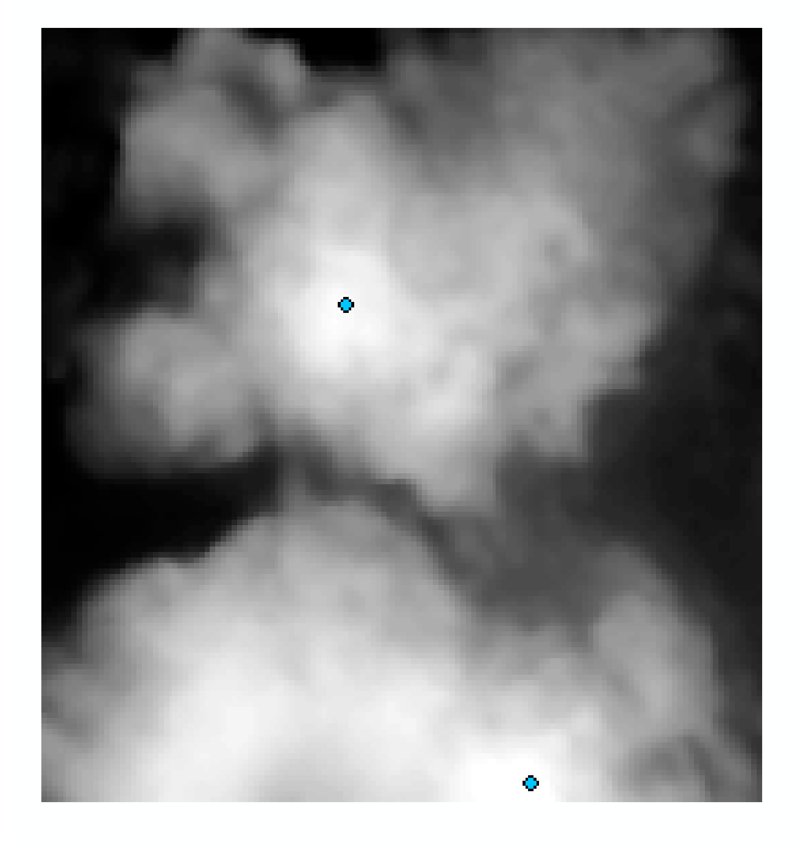
Figure 8.
Experimental results for Dataset 1: (a) DOM data for Dataset 1 (Jianzhou); (b) DEM data for Dataset 1 (Jianzhou); (c) Hillshading results for Dataset 1 (Jianzhou).
Figure 8.
Experimental results for Dataset 1: (a) DOM data for Dataset 1 (Jianzhou); (b) DEM data for Dataset 1 (Jianzhou); (c) Hillshading results for Dataset 1 (Jianzhou).
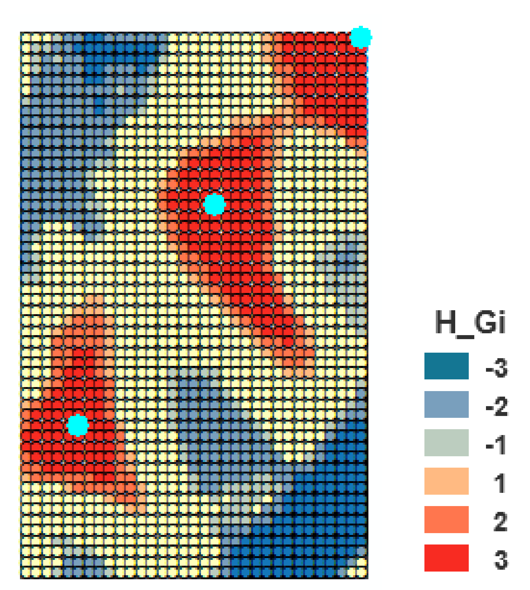
Figure 9.
The distribution map of the experimental first dataset extracted using the reference method.
Figure 9.
The distribution map of the experimental first dataset extracted using the reference method.
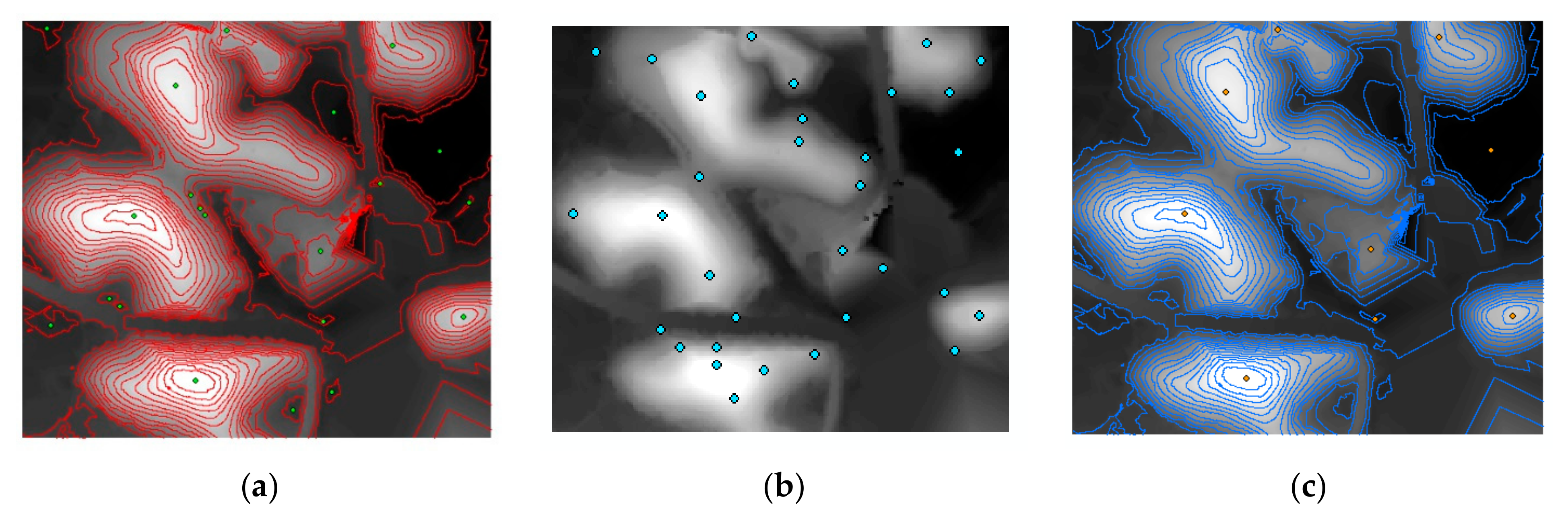
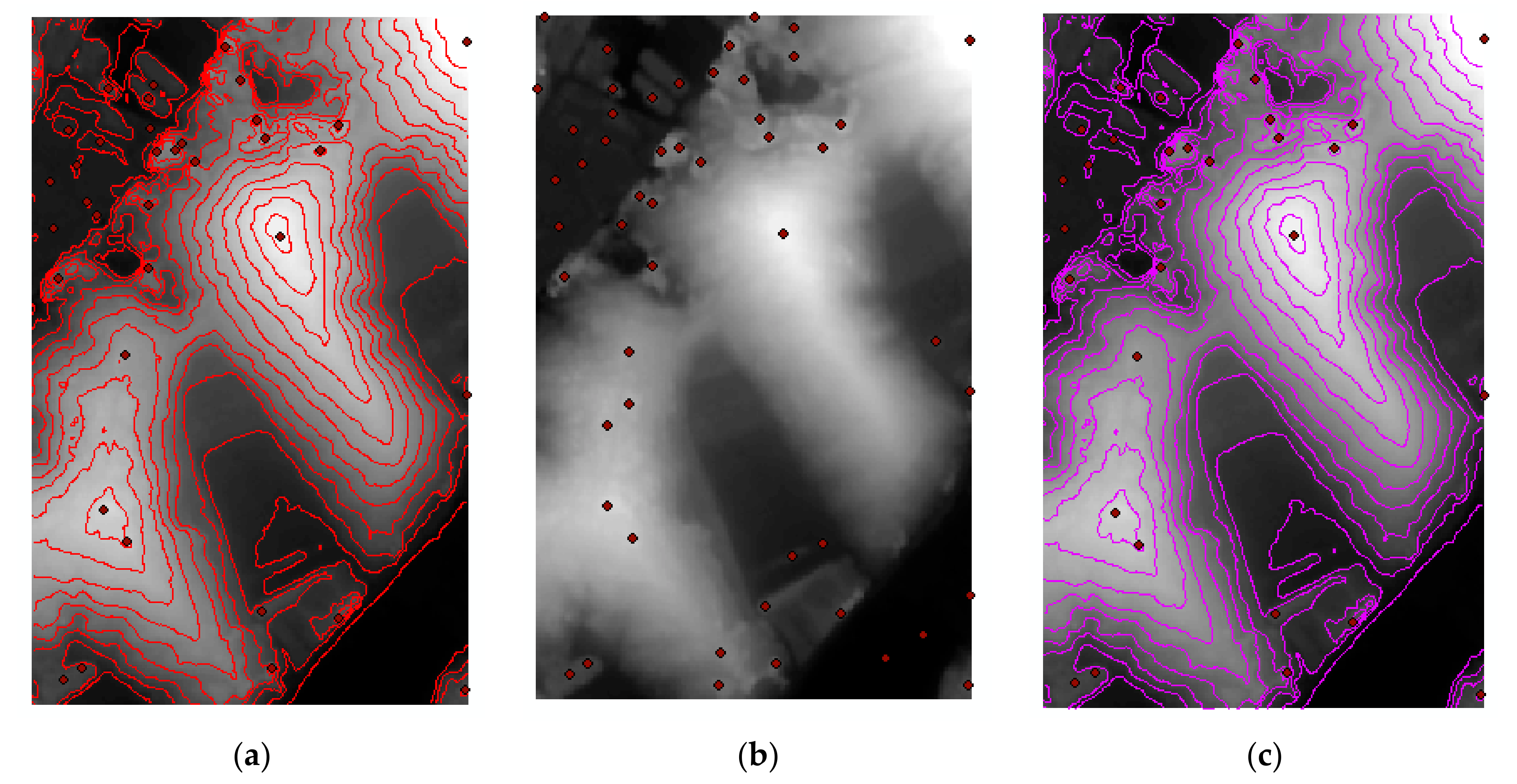
Figure 10.
The experimental first dataset distribution map extracted using traditional mountain vertex extraction methods: (a) Contour Line Method; (b) Neighborhood Analysis Method; and (c) Contour line and Neighborhood Analysis Overlay Method.
Figure 10.
The experimental first dataset distribution map extracted using traditional mountain vertex extraction methods: (a) Contour Line Method; (b) Neighborhood Analysis Method; and (c) Contour line and Neighborhood Analysis Overlay Method.
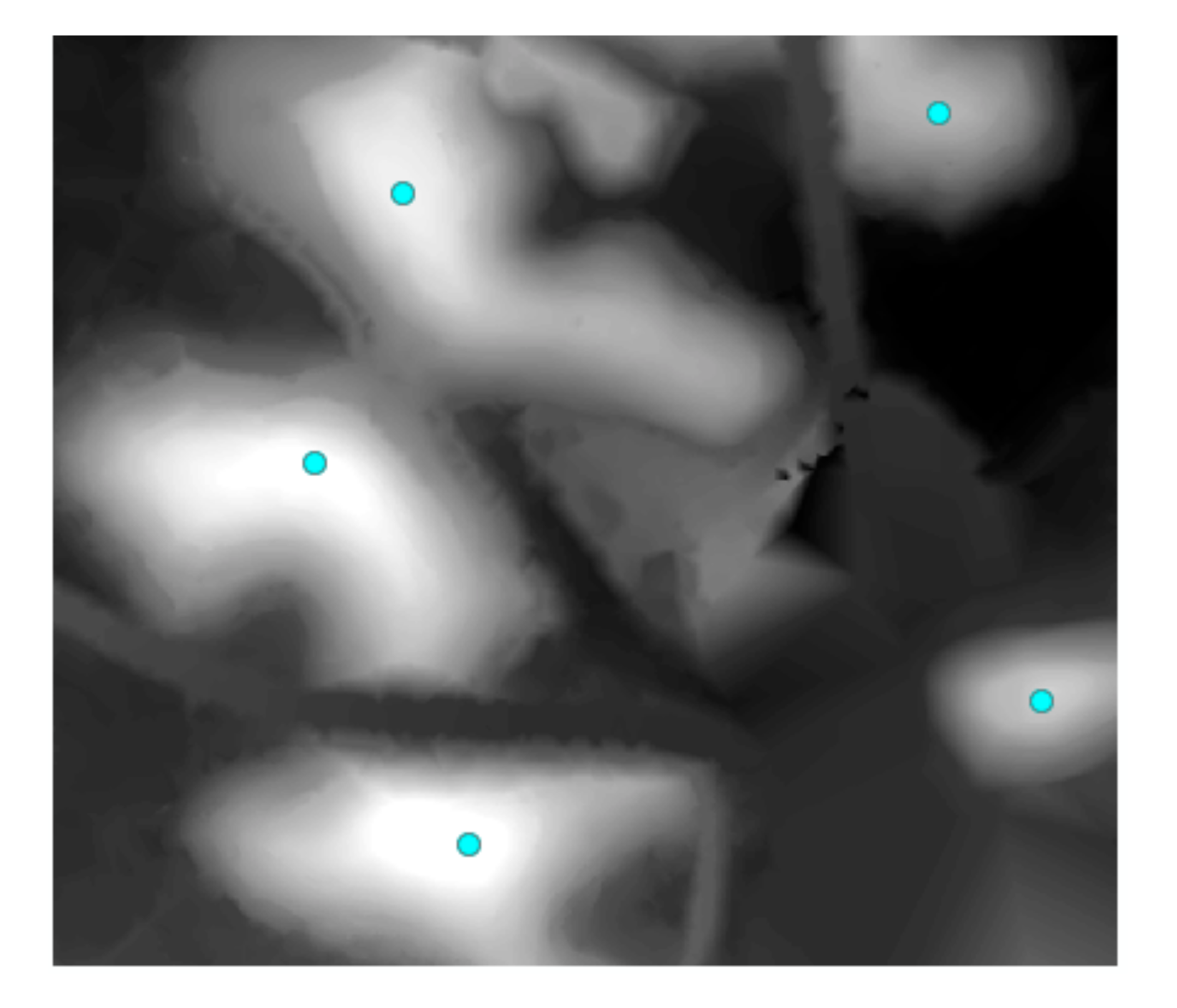
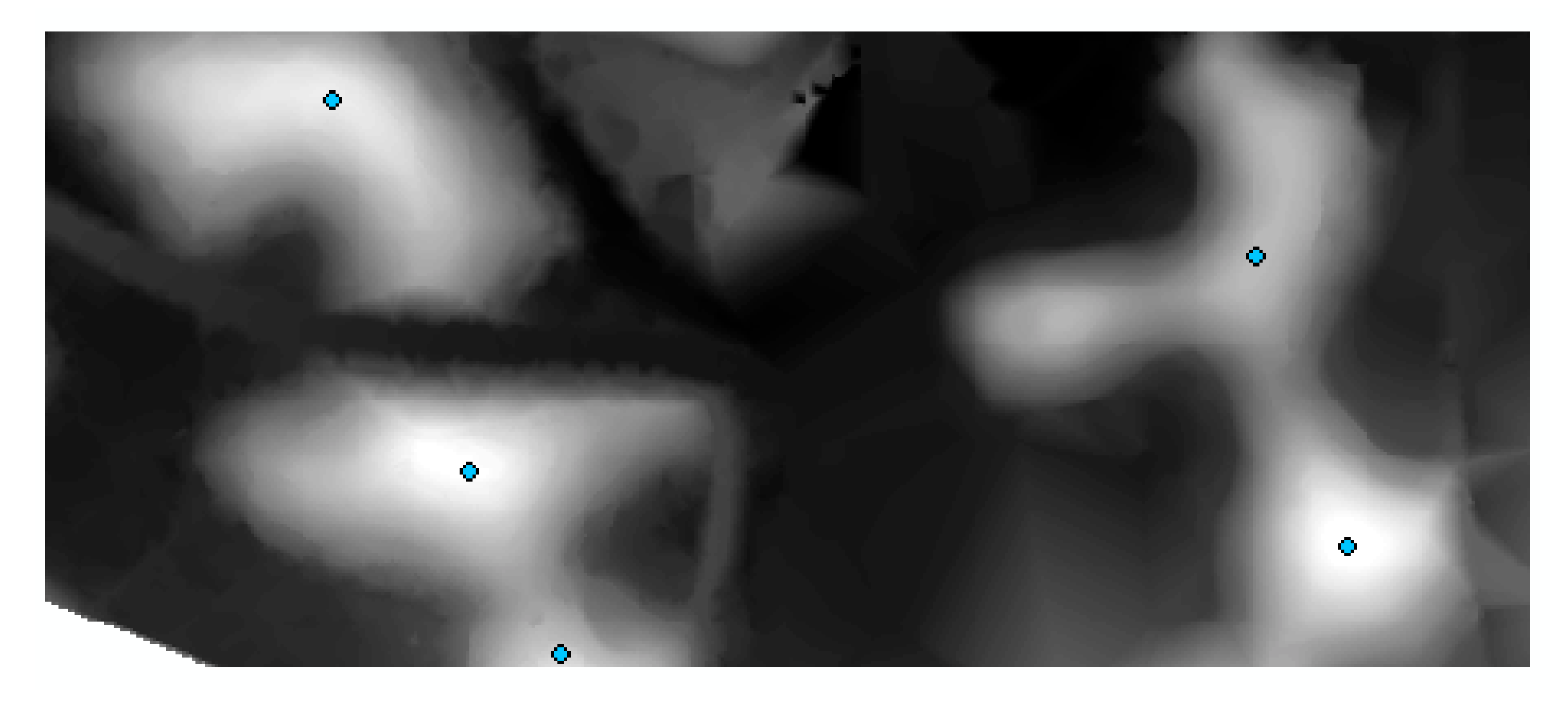
Figure 11.
The distribution map for the first dataset using our proposed approach.
Figure 11.
The distribution map for the first dataset using our proposed approach.
Figure 12.
The experimental second dataset: (a) DOM data of the second dataset (Jianzhou); (b) DEM data of the second dataset (Jianzhou); (c) Hillshading result of the second dataset (Jianzhou).
Figure 12.
The experimental second dataset: (a) DOM data of the second dataset (Jianzhou); (b) DEM data of the second dataset (Jianzhou); (c) Hillshading result of the second dataset (Jianzhou).
Figure 13.
The distribution map of the second dataset extracted using the reference method.
Figure 13.
The distribution map of the second dataset extracted using the reference method.
Figure 14.
Distribution maps extracted by the traditional Mountain Vertices Extraction Methods using the second dataset. (a) Contour Line Method. (b) Neighborhood Analysis Method. (c) Contour line and Neighborhood Analysis Overlay Method.
Figure 14.
Distribution maps extracted by the traditional Mountain Vertices Extraction Methods using the second dataset. (a) Contour Line Method. (b) Neighborhood Analysis Method. (c) Contour line and Neighborhood Analysis Overlay Method.
Figure 15.
The distribution map for the second dataset using our proposed approach.
Figure 15.
The distribution map for the second dataset using our proposed approach.
Figure 16.
The third dataset: (a) DOM data of the third dataset (the northern part of Nanyang, China); (b) DEM data of the third dataset (the northern part of Nanyang, China); (c) Hillshading result of the third dataset (the northern part of Nanyang, China).
Figure 16.
The third dataset: (a) DOM data of the third dataset (the northern part of Nanyang, China); (b) DEM data of the third dataset (the northern part of Nanyang, China); (c) Hillshading result of the third dataset (the northern part of Nanyang, China).
Figure 17.
The distribution map of the third dataset extracted using the reference method.
Figure 17.
The distribution map of the third dataset extracted using the reference method.
Figure 18.
Distribution maps extracted by the traditional Mountain Vertices Extraction Methods using the third dataset. (a) Contour Line Method. (b) Neighborhood Analysis Method. (c) Contour line and Neighborhood Analysis Overlay Method.
Figure 18.
Distribution maps extracted by the traditional Mountain Vertices Extraction Methods using the third dataset. (a) Contour Line Method. (b) Neighborhood Analysis Method. (c) Contour line and Neighborhood Analysis Overlay Method.
Figure 19.
The distribution map for the third dataset using our proposed approach.
Figure 19.
The distribution map for the third dataset using our proposed approach.
Figure 20.
The fourth dataset: (a) DOM data of the fourth dataset (the southern part of Nanyang, China); (b) DEM data of the fourth dataset (the southern part of Nanyang, China); (c) Hillshading result of the fourth dataset (the southern part of the Nanyang, China).
Figure 20.
The fourth dataset: (a) DOM data of the fourth dataset (the southern part of Nanyang, China); (b) DEM data of the fourth dataset (the southern part of Nanyang, China); (c) Hillshading result of the fourth dataset (the southern part of the Nanyang, China).
Figure 21.
The distribution map of the fourth dataset extracted using the reference method.
Figure 21.
The distribution map of the fourth dataset extracted using the reference method.
Figure 22.
Distribution maps extracted by the traditional Mountain Vertices Extraction Methods using the fourth dataset. (a) Contour Line Method. (b) Neighborhood Analysis Method. (c) Contour line and Neighborhood Analysis Overlay Method.
Figure 22.
Distribution maps extracted by the traditional Mountain Vertices Extraction Methods using the fourth dataset. (a) Contour Line Method. (b) Neighborhood Analysis Method. (c) Contour line and Neighborhood Analysis Overlay Method.
Figure 23.
The distribution map for the fourth dataset using our proposed approach.
Figure 23.
The distribution map for the fourth dataset using our proposed approach.
Figure 24.
The experimental fifth dataset: (a) DOM data of the fifth dataset (the eastern part of Ji’an, China); (b) DEM data of the fifth dataset (the eastern part of Ji’an, China); (c) hillshading result of the fifth dataset (the eastern part of Ji’an, China).
Figure 24.
The experimental fifth dataset: (a) DOM data of the fifth dataset (the eastern part of Ji’an, China); (b) DEM data of the fifth dataset (the eastern part of Ji’an, China); (c) hillshading result of the fifth dataset (the eastern part of Ji’an, China).
Figure 25.
The distribution map of the fifth dataset extracted using the reference method.
Figure 25.
The distribution map of the fifth dataset extracted using the reference method.
Figure 26.
Distribution maps extracted by the traditional Mountain Vertices Extraction Methods using the fifth dataset. (a) Contour Line Method. (b) Neighborhood Analysis Method. (c) Contour line and Neighborhood Analysis Overlay Method.
Figure 26.
Distribution maps extracted by the traditional Mountain Vertices Extraction Methods using the fifth dataset. (a) Contour Line Method. (b) Neighborhood Analysis Method. (c) Contour line and Neighborhood Analysis Overlay Method.
Figure 27.
The distribution map for the fifth dataset using our proposed approach.
Figure 27.
The distribution map for the fifth dataset using our proposed approach.
Figure 28.
The experimental sixth dataset:(a) DOM data of the sixth dataset (western part of Ji’an, China); (b) DEM data of the sixth dataset (western part of Ji’an, China); (c) Hillshading result of the sixth dataset (western part of Ji’an, China).
Figure 28.
The experimental sixth dataset:(a) DOM data of the sixth dataset (western part of Ji’an, China); (b) DEM data of the sixth dataset (western part of Ji’an, China); (c) Hillshading result of the sixth dataset (western part of Ji’an, China).
Figure 29.
The distribution map of the sixth dataset extracted using the reference method.
Figure 29.
The distribution map of the sixth dataset extracted using the reference method.
Figure 30.
Distribution maps extracted by the traditional Mountain Vertices Extraction Methods using the sixth dataset. (a) Contour Line Method. (b) Neighborhood Analysis Method. (c) Contour line and Neighborhood Analysis Overlay Method.
Figure 30.
Distribution maps extracted by the traditional Mountain Vertices Extraction Methods using the sixth dataset. (a) Contour Line Method. (b) Neighborhood Analysis Method. (c) Contour line and Neighborhood Analysis Overlay Method.
Figure 31.
The distribution map for the sixth dataset using our proposed approach.
Figure 31.
The distribution map for the sixth dataset using our proposed approach.
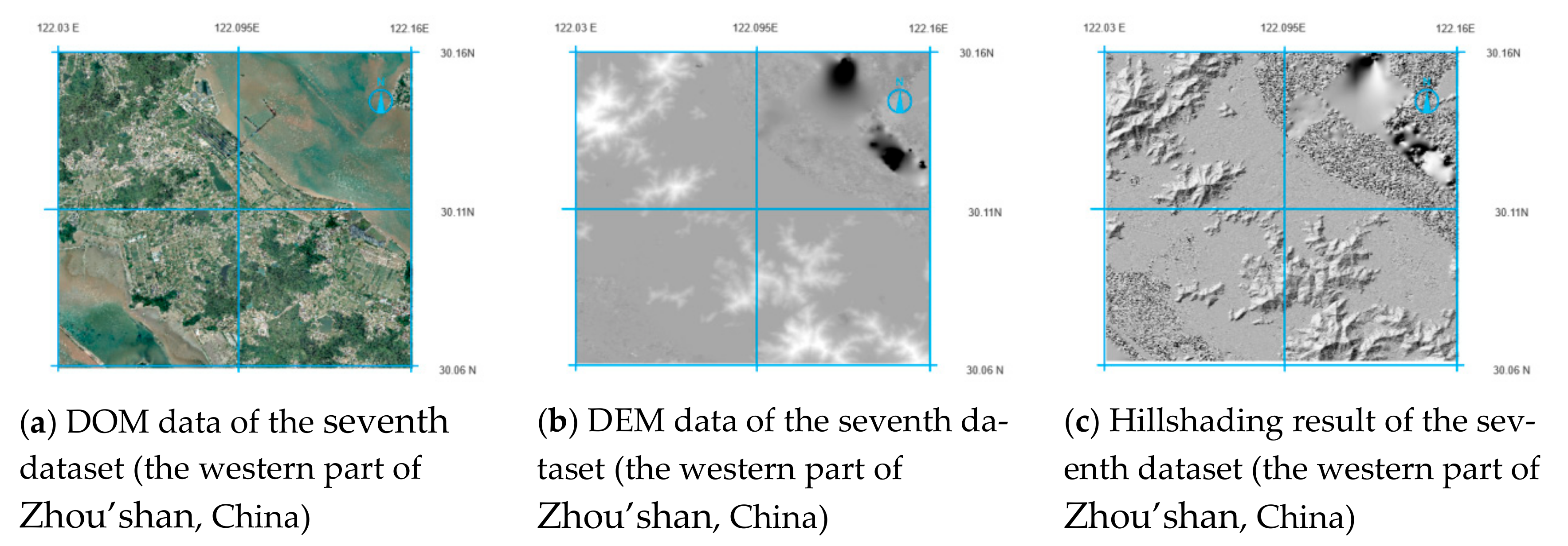
Figure 32.
The experimental seventh dataset:(a) DOM data of the seventh dataset (western part of Zhou’shan, China); (b) DEM data of the seventh dataset (western part of Zhou’shan, China); (c) Hillshading result of the seventh dataset (western part of Zhou’shan, China).
Figure 32.
The experimental seventh dataset:(a) DOM data of the seventh dataset (western part of Zhou’shan, China); (b) DEM data of the seventh dataset (western part of Zhou’shan, China); (c) Hillshading result of the seventh dataset (western part of Zhou’shan, China).
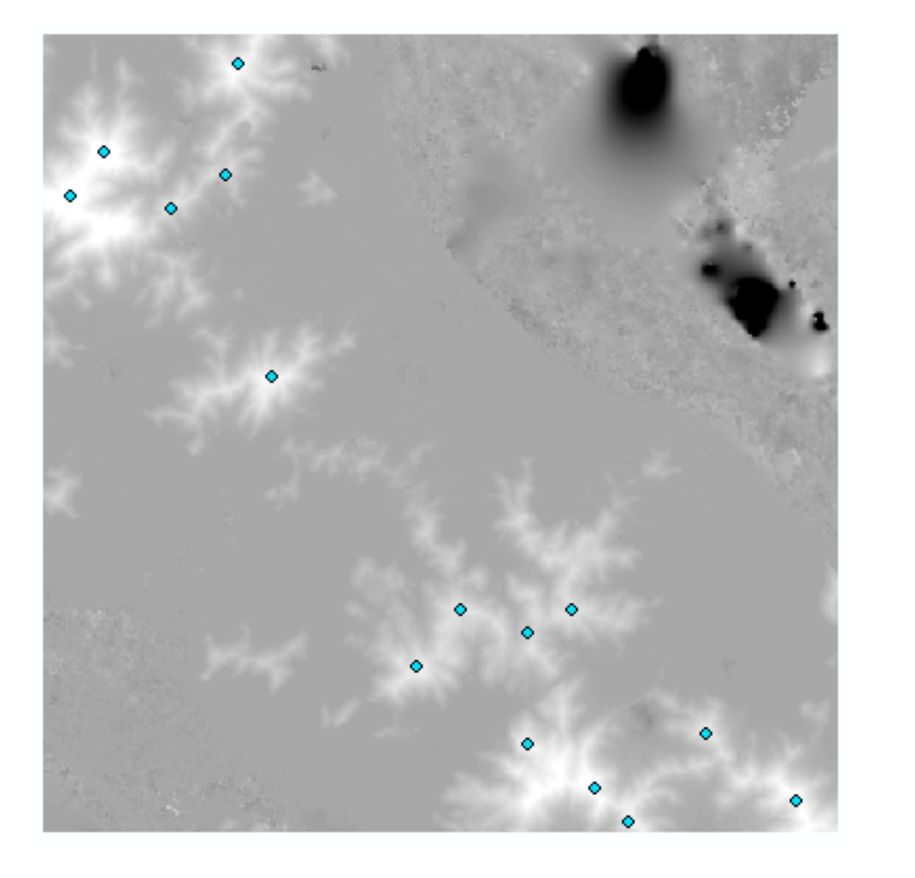
Figure 33.
The distribution map of the seventh dataset extracted using the reference method.
Figure 33.
The distribution map of the seventh dataset extracted using the reference method.
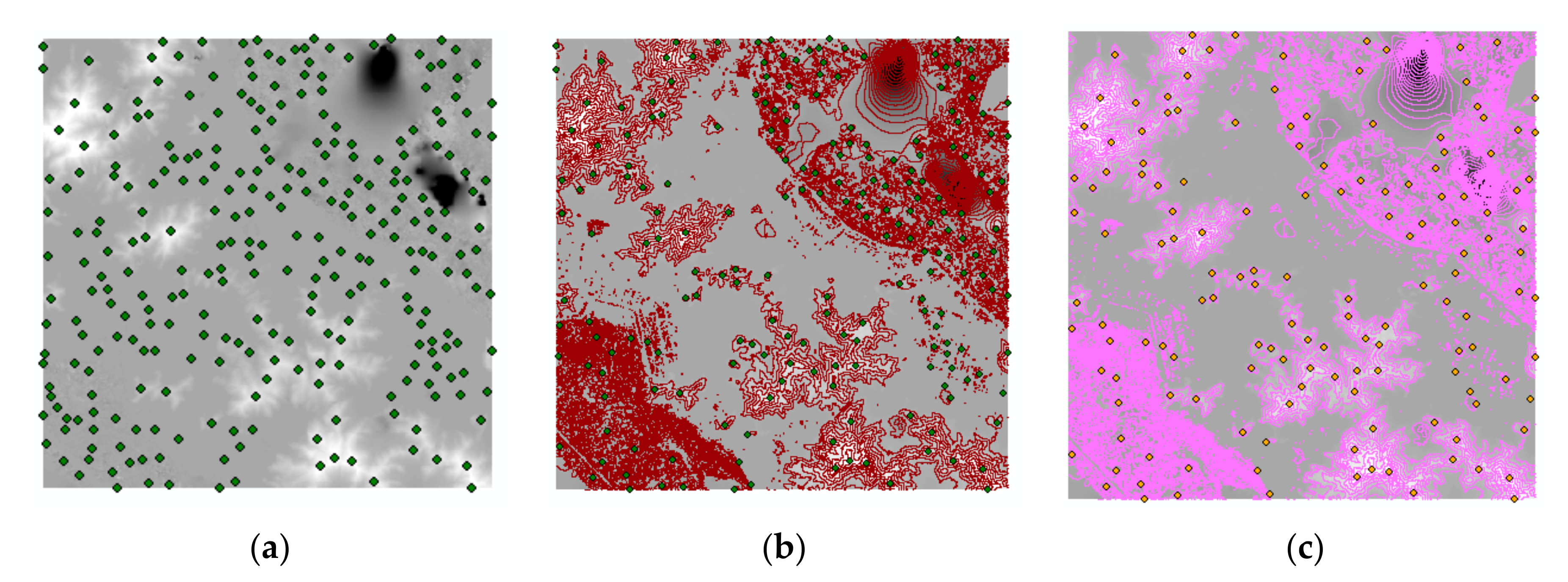
Figure 34.
Distribution maps extracted by the traditional Mountain Vertices Extraction Methods using the seventh dataset. (a) Contour Line Method. (b) Neighborhood Analysis Method. (c) Contour line and Neighborhood Analysis Overlay Method.
Figure 34.
Distribution maps extracted by the traditional Mountain Vertices Extraction Methods using the seventh dataset. (a) Contour Line Method. (b) Neighborhood Analysis Method. (c) Contour line and Neighborhood Analysis Overlay Method.
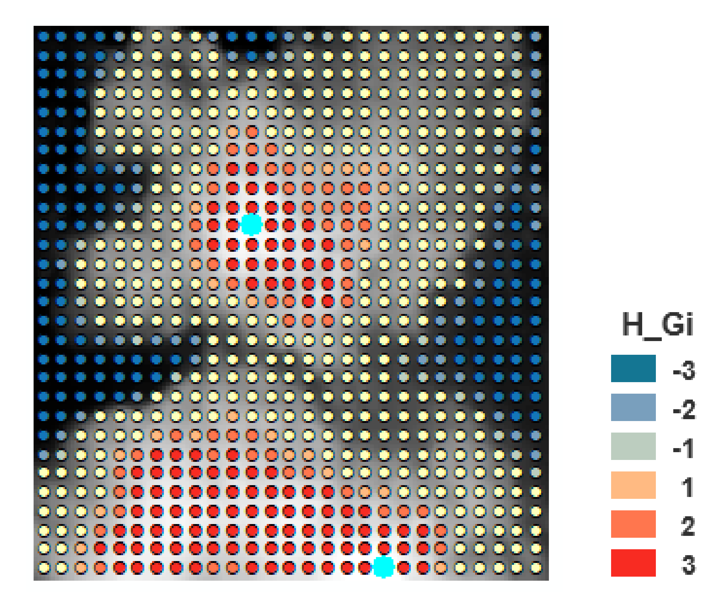
Figure 35.
The distribution map for the seventh dataset using our proposed approach.
Figure 35.
The distribution map for the seventh dataset using our proposed approach.
Table 1.
The Correspondence between Z-score, p-value and the Confidence.
Table 1.
The Correspondence between Z-score, p-value and the Confidence.
| Z-Score | p-Value | Confidence |
|---|
| <−1.65 || >+1.65 | <0.10 | 90% |
| <−1.96 || >+1.96 | <0.05 | 95% |
| <−2.58 || >+2.58 | <0.01 | 99% |
Table 2.
The Correspondence between Z-score, p-value, Confidence, and the H_Gi value.
Table 2.
The Correspondence between Z-score, p-value, Confidence, and the H_Gi value.
| Z-Score | p-Value | Confidence | H_Gi |
|---|
| <−1.65 || >+1.65 | <0.10 | 90% | −1 || 1 |
| <−1.96 || >+1.96 | <0.05 | 95% | −2 || 2 |
| <−2.58 || >+2.58 | <0.01 | 99% | −3 || 3 |
Table 3.
The difference between the experimental data.
Table 3.
The difference between the experimental data.
| NO. | Data Location | Data Range | Data Type | Spatial Resolution | Data Height |
|---|
| 1 | Jianzhou | 104.10°E–104.16°E
30.60°N~30.66°N | Raster | 1 m | high mountain: 429 m~483 m |
| 2 | Jianzhou | 104.10°E~104.19°E
30.59°N~30.64°N | Raster | 1 m | high mountain: 430 m~485 m |
| 3 | Nanyang | 112.06°E–112.08°E
33.185°N~30.20°N | Raster | 2 m | middle mountain: 231 m~277 m |
| 4 | Nanyang | 112.06°E–112.07°E
33.12°N~30.16°N | Raster | 2 m | middle mountain: 237 m~280 m |
| 5 | Ji’an | 114.23°E–114.236°E
27.19°N~27.20°N | Raster | 2 m | low mountain: 66 m~105 m |
| 6 | Ji’an | 114.11°E–114.12°E
27.18°N~27.19°N | Raster | 2 m | low mountain: 59 m~106 m |
| 7 | Zhou’shan | 122.03°E–122.16°E
30.06°N~30.16°N | Raster | 2 m | high mountain: −888 m~522 m |
Table 4.
Vertex extraction results for each method using the experimental first dataset.
Table 4.
Vertex extraction results for each method using the experimental first dataset.
| Method | Extract NUM | Correct NUM | False NUM | Extract Rate | Correct Rate |
|---|
| Reference Method | 5 | 5 | 0 | 100% | 100% |
| The Proposed Method | 5 | 5 | 0 | 100% | 100% |
| CLM | 21 | 3 | 2 | 14% | 60% |
| NAM | 32 | 4 | 1 | 12.5% | 80% |
| CLaNAOM | 9 | 4 | 1 | 45% | 80% |
Table 5.
The time consumed in extracting mountain vertices for the first dataset using our proposed approach.
Table 5.
The time consumed in extracting mountain vertices for the first dataset using our proposed approach.
| NO. | Method | Time |
|---|
| 1 | Resampling of the raster DEM by 10 × 10 pixel-size | 1.5 s |
| 2 | Raster DEM conversion into point vector DEM | 1.5 s |
| 3 | Hotspot analysis of the point vector DEM | 3 s |
| 4 | Extraction of mountain vertices | 4 s |
| | Total Time | 10 s |
Table 6.
The time spent in extracting mountain vertices for the first dataset using the Contour Line and Neighborhood Analysis Overlay Method.
Table 6.
The time spent in extracting mountain vertices for the first dataset using the Contour Line and Neighborhood Analysis Overlay Method.
| NO. | Method | Time |
|---|
| 1 | Set 6 × 6 analysis window to neighborhood analyze the Raster DEM image data | 6 s |
| 2 | Generate 3 m interval contour lines for DEM images, extract the innermost contour line area | 5.5 s |
| 3 | Calculate the intersection between the innermost circle of DEM and the neighborhood analysis obtain data to get the experimental first dataset’s Mountain Vertices | 3.5 s |
| | Total Time | 15 s |
Table 7.
The mountain vertices extraction results for each method using the second dataset.
Table 7.
The mountain vertices extraction results for each method using the second dataset.
| Method | Extract NUM | Correct NUM | False NUM | Extract Rate | Correct Rate |
|---|
| Reference Method | 5 | 5 | 0 | 100% | 100% |
| The Proposed Method | 5 | 5 | 0 | 100% | 100% |
| CLM | 16 | 3 | 2 | 19% | 60% |
| NAM | 27 | 4 | 1 | 15% | 80% |
| CLaNAOM | 12 | 4 | 1 | 33% | 80% |
Table 8.
The time consumed in extracting mountain vertices for the second dataset using our proposed approach.
Table 8.
The time consumed in extracting mountain vertices for the second dataset using our proposed approach.
| NO. | Method | Time |
|---|
| 1 | Resampling of the Raster DEM by 10 × 10 pixel-size | 1.1 s |
| 2 | Raster DEM conversion into point vector DEM | 1.2 s |
| 3 | Hotspot analysis of the Point Vector DEM | 2.7 s |
| 4 | Extraction of the mountain vertices | 3.6 s |
| | Total Time | 8.6 s |
Table 9.
The time spent in extracting mountain vertices for the second dataset using the Contour Line and Neighborhood Analysis Overlay Method.
Table 9.
The time spent in extracting mountain vertices for the second dataset using the Contour Line and Neighborhood Analysis Overlay Method.
| NO. | Method | Time |
|---|
| 1 | Set 6 × 6 analysis window to neighborhood analyze the Raster DEM image data | 5.3 s |
| 2 | Generate 3 m interval contour lines for DEM images, extract the innermost contour line area | 4.9 s |
| 3 | Calculate the intersection between the innermost circle of DEM and the neighborhood analysis obtain data to get the experimental second dataset’s Mountain Vertices | 3 s |
| | Total Time | 13.2 s |
Table 10.
The mountain vertices extraction results for each method using the third dataset.
Table 10.
The mountain vertices extraction results for each method using the third dataset.
| Method | Extract NUM | Correct NUM | False NUM | Extract Rate | Correct Rate |
|---|
| Reference Method | 5 | 5 | 0 | 100% | 100% |
| The Proposed Method | 5 | 5 | 0 | 100% | 100% |
| CLM | 41 | 3 | 2 | 7.3% | 60% |
| NAM | 63 | 4 | 1 | 6.3% | 80% |
| CLaNAOM | 34 | 4 | 1 | 11.8% | 80% |
Table 11.
The time consumed in extracting mountain vertices for the third dataset using our proposed approach.
Table 11.
The time consumed in extracting mountain vertices for the third dataset using our proposed approach.
| NO. | Method | Time |
|---|
| 1 | Resampling of the Raster DEM by 10 × 10 pixel-size | 0.21 s |
| 2 | Raster DEM conversion into point vector DEM | 0.26 s |
| 3 | Hotspot analysis of the Point Vector DEM | 0.33 s |
| 4 | Extraction of the mountain vertices | 0.45 s |
| | Total Time | 1.25 s |
Table 12.
The time spent in extracting mountain vertices for the third dataset using the Contour Line and Neighborhood Analysis Overlay Method.
Table 12.
The time spent in extracting mountain vertices for the third dataset using the Contour Line and Neighborhood Analysis Overlay Method.
| NO. | Method | Time |
|---|
| 1 | Set 6 × 6 analysis window to neighborhood analyze the Raster DEM data | 0.59 s |
| 2 | Generate 3 m interval contour lines for DEM data, extract the innermost contour line area | 0.54 s |
| 3 | Calculate the intersection between the innermost circle of DEM and the neighborhood analysis obtain data to get the experimental third dataset’s Mountain Vertices | 0.34 s |
| | Total Time | 1.47 s |
Table 13.
The mountain vertices extraction results for each method using the fourth dataset.
Table 13.
The mountain vertices extraction results for each method using the fourth dataset.
| Method | Extract NUM | Correct NUM | False NUM | Extract Rate | Correct Rate |
|---|
| Reference Method | 3 | 3 | 0 | 100% | 100% |
| The Proposed Method | 3 | 3 | 0 | 100% | 100% |
| CLM | 33 | 2 | 1 | 6% | 80% |
| NAM | 47 | 2 | 1 | 4.3% | 80% |
| CLaNAOM | 27 | 2 | 1 | 7.4% | 80% |
Table 14.
The time consumed in extracting mountain vertices for the fourth dataset using our proposed approach.
Table 14.
The time consumed in extracting mountain vertices for the fourth dataset using our proposed approach.
| NO. | Method | Time |
|---|
| 1 | Resampling of the Raster DEM by 10 × 10 pixel-size | 0.23 s |
| 2 | Raster DEM conversion into point vector DEM | 0.29 s |
| 3 | Hotspot analysis of the Point Vector DEM | 0.36 s |
| 4 | Extraction of the mountain vertices | 0.50 s |
| | Total Time | 1.38 s |
Table 15.
The time spent in extracting mountain vertices for the fourth dataset using the Contour Line and Neighborhood Analysis Overlay Method.
Table 15.
The time spent in extracting mountain vertices for the fourth dataset using the Contour Line and Neighborhood Analysis Overlay Method.
| NO. | Method | Time |
|---|
| 1 | Set 6 × 6 analysis window to neighborhood analyze the Raster DEM data | 0.65 s |
| 2 | Generate 3 m interval contour lines for DEM data, extract the innermost contour line area | 0.59 s |
| 3 | Calculate the intersection between the innermost circle of DEM and the neighborhood analysis obtain data to get the experimental fourth dataset’s Mountain Vertices | 0.37 s |
| | Total Time | 1.61 s |
Table 16.
The mountain vertices extraction results for each method using the fifth dataset.
Table 16.
The mountain vertices extraction results for each method using the fifth dataset.
| Method | Extract NUM | Correct NUM | False NUM | Extract Rate | Correct Rate |
|---|
| Reference Method | 2 | 2 | 0 | 100% | 100% |
| The Proposed Method | 2 | 2 | 0 | 100% | 100% |
| CLM | 15 | 2 | 1 | 13% | 50% |
| NAM | 18 | 2 | 0 | 11% | 100% |
| CLaNAOM | 12 | 2 | 0 | 16% | 100% |
Table 17.
The time consumed in extracting mountain vertices for the fifth dataset using our proposed approach.
Table 17.
The time consumed in extracting mountain vertices for the fifth dataset using our proposed approach.
| NO. | Method | Time |
|---|
| 1 | Resampling of the Raster DEM by 10 × 10 pixel-size | 0.08 s |
| 2 | Raster DEM conversion into point vector DEM | 0.09 s |
| 3 | Hotspot analysis of the Point Vector DEM | 0.12 s |
| 4 | Extraction of the mountain vertices | 0.16 s |
| | Total Time | 0.45 s |
Table 18.
The time spent in extracting mountain vertices for the fifth dataset using the Contour Line and Neighborhood Analysis Overlay Method.
Table 18.
The time spent in extracting mountain vertices for the fifth dataset using the Contour Line and Neighborhood Analysis Overlay Method.
| NO. | Method | Time |
|---|
| 1 | Set 6 × 6 analysis window to neighborhood analyze the Raster DEM data | 0.21 s |
| 2 | Generate 3 m interval contour lines for DEM data, extract the innermost contour line area | 0.19 s |
| 3 | Calculate the intersection between the innermost circle of DEM and the neighborhood analysis obtain data to get the experimental fifth dataset’s Mountain Vertices | 0.12 s |
| | Total Time | 0.52 s |
Table 19.
The mountain vertices extraction results for each method using the sixth dataset.
Table 19.
The mountain vertices extraction results for each method using the sixth dataset.
| Method | Extract NUM | Correct NUM | False NUM | Extract Rate | Correct Rate |
|---|
| The Reference Method | 2 | 2 | 0 | 100% | 100% |
| The Proposed Method | 2 | 2 | 0 | 100% | 100% |
| CLM | 14 | 2 | 0 | 14% | 100% |
| NAM | 19 | 2 | 0 | 11% | 100% |
| CLaNAOM | 11 | 2 | 0 | 18% | 100% |
Table 20.
The time consumed in extracting mountain vertices for the sixth dataset using our proposed approach.
Table 20.
The time consumed in extracting mountain vertices for the sixth dataset using our proposed approach.
| NO. | Method | Time |
|---|
| 1 | Resampling of the Raster DEM by 10 × 10 pixel-size | 0.11 s |
| 2 | Raster DEM conversion into point vector DEM | 0.13 s |
| 3 | Hotspot analysis of the Point Vector DEM | 0.17 s |
| 4 | Extraction of the mountain vertices | 0.22 s |
| | Total Time | 0.63 s |
Table 21.
The time spent in extracting mountain vertices for the sixth dataset using the Contour Line and Neighborhood Analysis Overlay Method.
Table 21.
The time spent in extracting mountain vertices for the sixth dataset using the Contour Line and Neighborhood Analysis Overlay Method.
| NO. | Method | Time |
|---|
| 1 | Set 6 × 6 analysis window to neighborhood analyze the Raster DEM data | 0.29 s |
| 2 | Generate 3 m interval contour lines for DEM data, extract the innermost contour line area | 0.27 s |
| 3 | Calculate the intersection between the innermost circle of DEM and the neighborhood analysis obtain data to get the experimental sixth dataset’s mountain vertices | 0.17 s |
| | Total Time | 0.73 s |
Table 22.
The mountain vertices extraction results for each method using the seventh dataset.
Table 22.
The mountain vertices extraction results for each method using the seventh dataset.
| Method | Extract NUM | Correct NUM | False NUM | Extract Rate | Correct Rate |
|---|
| The Reference Method | 15 | 15 | 0 | 100% | 100% |
| The Proposed Method | 15 | 15 | 0 | 100% | 100% |
| CLM | 180 | 12 | 3 | 7% | 80% |
| NAM | 240 | 13 | 2 | 5% | 87% |
| CLaNAOM | 120 | 13 | 2 | 11% | 87% |
Table 23.
The time consumed in extracting mountain vertices for the seventh dataset using our proposed approach.
Table 23.
The time consumed in extracting mountain vertices for the seventh dataset using our proposed approach.
| NO. | Method | Time |
|---|
| 1 | Resampling of the Raster DEM by 10 × 10 pixel-size | 14.4 s |
| 2 | Raster DEM conversion into point vector DEM | 14 s |
| 3 | Hotspot analysis of the Point Vector DEM | 28.6 s |
| 4 | Extraction of the mountain vertices | 38.6 s |
| | Total Time | 95.6 s |
Table 24.
The time spent in extracting mountain vertices for the seventh dataset using the Contour Line and Neighborhood Analysis Overlay Method.
Table 24.
The time spent in extracting mountain vertices for the seventh dataset using the Contour Line and Neighborhood Analysis Overlay Method.
| NO. | Method | Time |
|---|
| 1 | Set 6 × 6 analysis window to neighborhood analyze the Raster DEM data | 58.2 s |
| 2 | Generate 3 m interval contour lines for DEM data, extract the innermost contour line area | 53.4 s |
| 3 | Calculate the intersection between the innermost circle of DEM and the neighborhood analysis obtain data to get the experimental seventh dataset’s mountain vertices | 34.1 s |
| | Total Time | 145.7 s |
Table 25.
The extraction rate in each method for Datasets 1–7.
Table 25.
The extraction rate in each method for Datasets 1–7.
| Method | Dataset-1 | Dataset-2 | Dataset-3 | Dataset-4 | Dataset-5 | Dataset-6 | Dataset-7 |
|---|
| The Proposed Method | 100% | 100% | 100% | 100% | 100% | 100% | 100% |
| CLM | 14% | 19% | 7.3% | 6% | 13% | 14% | 7% |
| NAM | 12.5% | 15% | 6.3% | 4.3% | 11% | 11% | 5% |
| CLaNAOM | 45% | 33% | 11.8% | 7.4% | 16% | 18% | 11% |
Table 26.
The accuracy rate for each method using in the first to seventh dataset to extract the mountain vertices.
Table 26.
The accuracy rate for each method using in the first to seventh dataset to extract the mountain vertices.
| Method | Dataset-1 | Dataset-2 | Dataset-3 | Dataset-4 | Dataset-5 | Dataset-6 | Dataset-7 |
|---|
| The Proposed Method | 100% | 100% | 100% | 100% | 100% | 100% | 100% |
| CLM | 60% | 60% | 60% | 80% | 50% | 100% | 80% |
| NAM | 80% | 80% | 80% | 80% | 100% | 100% | 87% |
| CLaNAOM | 80% | 80% | 80% | 80% | 100% | 100% | 87% |


 ,
, 


