Abstract
Soil moisture is the most active part of the terrestrial water cycle, and it is a key variable that affects hydrological, bio-ecological, and bio-geochemical processes. Microwave remote sensing is an effective means of monitoring soil moisture, but the existing conventional radiometers and single-station radars cannot meet the scientific needs in terms of temporal and spatial resolution. The emergence of GNSS-R (Global Navigation Satellite Systems Reflectometry) technology provides an alternative method with high temporal and spatial resolution. An important application field of GNSS-R is soil moisture monitoring, but it is still in the initial stage of research, and there are many uncertainties and open issues. Based on a review of the current state-of-the-art of soil moisture retrieval using GNSS-R, this paper points out the limitations of existing research in observation geometry, polarization, and coherent and non-coherent scattering. The smooth surface reflectivity model, the random rough surface scattering model, and the first-order radiation transfer equation model of the vegetation, which are in the form of bistatic and full polarization, are employed. Simulations and analyses of polarization, observation geometry (scattering zenith angle and scattering azimuth angle), Brewster angle, coherent and non-coherent component, surface roughness, and vegetation effects are carried out. The influence of the EIRP (Effective Isotropic Radiated Power) and the RFI (Radio Frequency Interference) on soil moisture retrieval is briefly discussed. Several important development directions for space-borne GNSS-R soil moisture retrieval are pointed out in detail based on the microwave scattering model.
Keywords:
soil moisture; GNSS-R; polarization; observation geometry; coherent and non-coherent; EIRP; RFI 1. Introduction
Soil moisture refers to the water content of the unsaturated layer of soil (also called the seepage layer). Soil moisture is the most active part of the terrestrial water cycle, and it is a key variable that affects hydrological, bio-ecological, and bio-geochemical processes. It especially plays an important role in surface water evapotranspiration and seepage. Soil moisture is also a link between surface water and groundwater and it is an important part of terrestrial ecosystems and water circulation systems. As one of the determinants of the state of the terrestrial hydrosphere, soil moisture largely controls the land surface evapotranspiration, water migration, and carbon cycle. Soil moisture can be used to understand and predict climate change, global water cycle, water resources management, and watershed hydrology. Soil moisture monitoring plays an important role in improving model forecasts of regional and global climate, environmental disasters, and other related natural and ecological environmental issues [1,2,3,4].
Time Domain Reflectometry (TDR) uses the soil reflection in the time domain to estimate soil moisture content. However, this technique is very limited when dealing with large-scale monitoring due to its uneven distribution on the Earth’s surface, and it is only used at a regional scale [5]. Other traditional observation methods mainly use discrete observations from meteorological stations, which can only sense a limited area (~10–100 cm). In addition, these traditional techniques are time-consuming, labor-intensive, and cannot meet the needs of large-scale, homogeneous-coverage, and high-efficiency soil moisture monitoring.
Fortunately, the recent advances in remote sensing technology have proposed a new methodology for obtaining soil moisture measurements at a large scale. Microwave remote sensing employs the soil permittivity (ε) properties to obtain soil moisture. The values of dry (ε = 5) and wet (ε = 80) soil usually are very large, and the L-band is considered the best band for soil moisture monitoring [6].
Traditional radiometers use the electromagnetic signal radiated by the ground, from which geophysical parameters can be estimated, including, e.g., the surface brightness temperature and the soil moisture content. Traditional radiometers usually provide a low time resolution (2 to 3 days) and are not sensitive to surface roughness. However, these measurements are strongly sensitive to background brightness temperature and artificial radio frequency interferences (RFI). At present, two passive microwave radiometers, SMOS (Soil Moisture and Ocean Salinity) from the European Space Agency (ESA) and SMAP (Soil Moisture Active and Passive) from the National Aeronautics and Space Administration (NASA), have been provided measurements since 2009 and 2015, respectively, with a spatial resolution of ~40 km, and a temporal resolution of two to three days [7,8,9]. Nowadays, these are the main sources for large-scale soil moisture monitoring.
Compared to radiometers, monostatic radars that emit microwave signals can also be employed to sense the backscattered signal, and then use that information to retrieve geophysical parameters. Soil moisture is one of the most important parameters that affect the final backscattering signals. This technique can provide sub-kilometer spatial resolution and is easily affected by surface characteristics, such as surface roughness, soil dielectric constant, and vegetation structure. However, this technique has complex data processing, a lower temporal resolution than radiometers, and a very high instrumental cost [7].
Recently, bistatic radars have been proposed as an emerging technology to estimate soil moisture monitoring. This new technique requires heavy and expensive transmitters and economic and low-power consumption receivers. In recent years, Global Navigation Satellite Systems (GNSS) reflected signals have shown the potential capability of the new GNSS reflectometry (GNSS-R) technology [10,11,12]. GNSS-R technology uses the existing navigation satellite constellations as signal transmitters, and only needs a special receiver on-board numerous kinds of platforms, such as CubeSats or airplanes, to collect the reflected signals. This technique can provide measurements at a high spatial and temporal resolution, and it is an effective supplement to existing observational methods. Moreover, the continuous increase in existing direct signal sources results in an increase in the sampling frequency of surface reflection data, and thus reducing the revisit period.
The earliest work of GNSS-R for soil moisture monitoring was a Master’s thesis [13]. Many studies have employed information on multipath effects from ground-based GNSS receivers to retrieve soil moisture [14,15,16,17]. In addition, in the past years, several airborne experiments have been carried out to monitor soil moisture using GNSS-R [18,19].
In terms of spaceborne observations, the UK-DMC (United Kingdom-Disaster Monitoring Constellation) and the TDS-1 (TechDemoSat-1) satellite tests were launched in 2004 and 2014, respectively [20,21]. In December 2016, the CYGNSS (Cyclone Global Navigation Satellite System) was successfully launched, to measure wind field information on the ocean surface during tropical storms and hurricanes. Fortunately, it also provides an important opportunity for land surface and cryosphere monitoring [22,23]. In June 2019, Bufeng-1 A and B satellites were successfully deployed for sea-surface wind monitoring [24]. Moreover, in December 2019, two GNSS-R CubeSats were launched with the Indian Polar Orbiting Satellite Carrier (PSLV) rocket, for studies of soil moisture and sea breeze, and the payload GNOS II (Global Navigation Satellite System Occultation Sounder II) of the National Space Science Center of the Chinese Academy of Sciences (NSSCCAS) is expected to start on 2020 (E satellite of the FY-3 meteorological satellite) [25].
Although most of these space-borne satellite missions are currently mainly used for sea surface monitoring, their development has also opened a door for land surface studies, more specifically, soil moisture monitoring, which is a very important application for spaceborne GNSS-R. This paper will give a review of the inversion technique for CYGNSS data, and carry out corresponding simulations according to the existing problems for soil moisture retrieval. Finally, we will discuss the potential development opportunities and challenges.
2. Research Status and Existing Problems
The available spaceborne GNSS-R programs for soil moisture detection mainly include UK-DMC, TDS-1, and CYGNSS. The UK-DMC is equipped with the first spaceborne GNSS-R receiver, which was originally used to study the ocean surface roughness and to estimate the sea surface wind speed. Later research found that the reflected signals from the land surface can also be received [20]. The TDS-1 satellite was successfully launched on 8 July 2014, with eight test payloads. The SGR-ReSI (Space GNSS Receiver Remote Sensing Instrument) onboard TDS-1 can provide a large amount of GNSS reflection data [21]. The TDS-1 data is very similar to the CYGNSS data. However, the amount of data collected by TDS-1 is several orders of magnitude smaller than that of CYGNSS, since the revisit time of TDS-1 is greater than 6 months, while that of CYGNSS about 1 day. Therefore, TDS-1 can only evaluate the spatial correspondence between GNSS reflected signals and soil moisture at a single moment, and it cannot obtain large time-series analysis results [26,27,28,29].
Here, the parameter of interest is the peak energy of the Delay-Doppler Map (DDM), which is not only affected by the nature of the reflecting surface, but also by the antenna gain, the transmitter and receiver ranges, and the incidence angle, as shown in [26] as:
In this equation, is the effective reflected energy, i.e., the signal-to-noise ratio (SNR) of the DDM. is the maximum reflected energy of DDM, is the receiver noise, and are the transmitter and receiver ranges, is the incidence angle, and is the antenna gain. The first paper using spaceborne GNSS-R for soil moisture research pointed out that the sensitivity of reflected signals to soil moisture changes is about 7 dB [26]. However, soil roughness and vegetation strongly affect the accuracy of the soil moisture estimates but, if these effects can be effectively solved, the resulting products can become a very valuable data-set at a high temporal and spatial resolution.
2.1. Soil Moisture Retrieval Using CYGNSS
There are several works done by [11,30,31,32,33,34] to retrieve soil moisture using CYGNSS. Chew’s work [30] specified a complete coherence from CYGNSS data for soil moisture retrieval. Kim and Yan’ works [31,34] assumed that the data is mainly coherent. Al-Khaldi [33] assumed that the energy is mainly non-coherent. Here, we summarize the current calculation methods of coherent and non-coherent terms [35] for CYGNSS data processing. The energy of the coherent scattering can be expressed as:
In this equation, is the transmitted power, is the wavelength, and are the antenna gain of the receiver and transmitter, respectively, and is the Fresnel reflection coefficient. The first exponential term is the coherent reflection loss (CRL), where is the free space wave number, is the surface roughness computed as Root Mean Square (RMS), and is the angle of incidence. The second exponential term is the attenuation due to vegetation, where is the vegetation optical depth (VOD).
On the other hand, the energy of the non-coherent scattering can be expressed as:
In this equation, is the non-coherent part of the received energy, where the time delay and the Doppler shift are and , respectively. is the bi-static radar cross-section. is the ambiguity function, is the individual surface point, and the DDM at the specular point () can be approximated as:
where the effective area is:
In [30], the observation angle is not specially processed. The SNR data of CYGNSS is compared to SMAP soil moisture data from March 2017 to February 2018. It was found that there is a strong positive linear correlation between the CYGNSS reflectivity and SMAP soil moisture. The authors established a linear regression between CYGNSS and SMAP data, with an RMS fit of 0.045 cm3/cm3. Their work indicates that CYGNSS can monitor soil moisture under medium vegetation coverage, but in drought and dense vegetation coverage, the results of soil moisture retrieval are poor. The results showed that CYGNSS and other future GNSS-R missions can be used to provide global soil moisture observations.
In [31], the authors assumed that the surface reflected signal received by CYGNSS is mainly coherent and, therefore, the calculation of the non-coherent scattering can be ignored. The incidence angle is considered during inversion, and it is normalized as:
In this equation, is the SNR for pixel (xi, yi) at the incidence angle . It can be normalized by the SNR data within the angle range of (35° ± 5°) in the same pixel, that is, is the normalized value at pixel . is the time average, is the standard deviation of the SNR during the study period. The authors used the relative SNR (rSNR) data from April 2017 to April 2018 for soil moisture inversion and assumed a linear correlation between rSNR and SMAP soil moisture (r = 0.68/0.77). By coupling rSNR and SMAP soil moisture data, the daily change of soil moisture can be obtained. Although the angle factor is considered, it is actually a simple normalization process. The scattering characteristics of soil moisture under different observation geometries have not been explored and fully used. The inversion algorithm based on different observation angles has not been established yet.
In [32], the authors assumed that the reflected signal of CYGNSSs is mainly coherent, used SMAP vegetation and soil roughness information as ancillary data, and employed CYGNSS data to retrieve pan-tropical soil moisture. A linear regression method was employed to estimate soil moisture as a function of SMAP VOD and surface roughness with an RMS of 0.07 cm3/cm3. One advantage of this retrieval method is that it can be applied to CYGNSS L2 data, which has higher resolution [32].
In [33], the authors pointed out that the coherent energy mainly comes from the specular reflection of inland water. This will cause the DDM peak value to increase, and the peak energy of the coherent part will be larger than the non-coherent part. Therefore, the method for soil moisture inversion might have unreliable results by only considering the coherent part of the reflection. In this way, [33] employed the non-coherent energy to retrieve soil moisture. There is a strong correlation between the coherent reflection WAF (Woodward Ambiguity Function) and the non-coherent reflection WAF. The method to remove the coherent term is to establish a correlation between the normalized BRCS (Bi-static Radar Cross Section) and the WAF. When the correlation is greater than the threshold, the DDM is considered to be the main component due to coherent scattering. In [33], the low SNR terms were also removed. The low SNR from land surface is mainly caused by the location of the image point in the CYGNSS antenna pattern (low scattering). Then, by setting the minimum threshold of SNR, the SNR term is removed. The calculation of land surface from non-coherent BRCS adopts the following form [33]:
In this equation, is the Fresnel coefficient, MSS is the mean square slope of surface roughness, and is the VOD.
Previous research [31,32,33] focused on a small incidence angle. However, the incidence angle of CYGNSS ranges between 0° and 70°, with a standard deviation of 16.7°. In order to improve data quality, CYGNSS data with incidence angle values greater than 60° are eliminated. The literature had processed the influence of incident angle on soil moisture retrieval, where the reflectivity in the nadir angle direction is used for normalization [33]. Regarding the attenuation of vegetation, it is assumed that the attenuation due to VOD at different angles remains constant. The assumption was made during the inversion of soil moisture in [33], where the surface roughness changed slowly compared with the changes in vegetation and soil moisture. In the inversion, the soil moisture product of SMAP is generally used as a reference value. For instance, [34] established a linear regression between the CYGNSS reflectivity and the soil moisture and the VOD of SMAP. The authors showed that there was a good correlation between the inverted soil moisture and the ground truth value, with a correlation coefficient of 0.8, and a RMSE or 0.07 cm3/cm3. Compared with the soil moisture of SMAP, the spatial coverage rate of the pantropical area covered by CYGNSS increased by 22%. However, reducing the dependence on external soil moisture data is a very important aspect for GNSS-R. For instance, [11] retrieved soil moisture from CYGNSS coherent scattering by only estimating the dielectric permittivity from Fresnel reflection coefficients, and without any regression or fit to SMAP soil moisture data. The resulting values were compared to SMAP with a RMS error of 0.05 cm3/cm3. Therefore, it is assumed that the receiver mainly obtains the energy of coherent scattering.
2.2. Current Problems in CYGNSS Soil Moisture Retrieval
At present, the main problems in CYGNSS soil moisture retrieval are as follows.
2.2.1. Less Consideration on Observation Angles
CYGNSS has a very good spatial and temporal resolution, and the reliable amount of data can be increased by accounting for the effects of extreme incidence angles. In the literature, we can see that some authors [30,32,34] ignore the influence of incidence angle for soil moisture inversion, while others [11,31,33] account for normalization. The angle information in the observation geometry is usually not considered (such as incident angle, scattered zenith angle, and azimuth angle), while this can impact on the accuracy of the final estimates. The processing of the angles is an open issue in the current inversion of CYGNSS. In fact, the angle information in different observation geometries has a greater impact on the reflection coefficient or bi-static scattering coefficient. In Section 3, microwave scattering models will be used to simulate and analyze the scattering characteristics at different angles.
2.2.2. Fuzzy Calculations on Coherent and Non-Coherent Scattering
On the ocean surface, it is assumed that the received reflected signal is a non-coherent scattering. On the land surface, it is mainly considered that the energy received by the receiver is the forward coherent energy from the first Fresnel zone [31,34]. However, methods for threshold analysis of WAF and DDM have been studied recently, and these used the non-coherent parts for soil moisture inversion [33]. The processing of coherent and incoherent scattered energy of CYGNSS is currently an open issue. The actual surface is randomly rough, and it seems impossible that the incident signal is completely a specular coherent scattering. The scattered surface is randomly rough, and there might be parts of diffuse scattering energy. In Section 3, the microwave scattering model is used to simulate the coherent and non-coherent scattering.
2.2.3. Data Dependence in the Inversion Algorithm
There is a linear correlation between CYGNSS reflectivity and SMAP soil moisture. Some researchers use CYGNSS reflectivity, SMAP, VOD, and roughness coefficients to establish a statistical linear regression for soil moisture retrieval [30,31,32,33,34]. Meanwhile, SMAP soil moisture data is usually regarded as truth data, so it makes the inversion algorithm to be highly dependent on the ancillary data. To reduce the dependence on ancillary data is a very important direction for inversion algorithm development. More methods based on empirical and physical scattering models [11] should be developed for a realistic soil moisture inversion.
In general, the initial purpose of CYGNSS was monitoring ocean winds with a spatial resolution of 25 × 25 km. However, in recent years, many authors have provided higher resolution for other products, as for example the UCAR/CU with CYGNSS soil moisture product at a 6-h and at 0.5 × 3.5 km resolution (after July 2019, before was 0.5 × 7 km). In this field, there are many options for improvements, as for example, supplementing future missions with polar orbits. Note here that the geometry of GNSS-R versus the traditional SAR has not been fully exploited.
Notwithstanding, an important point to improve is the dependence on auxiliary data, including bare soil roughness, vegetation optical depth, etc. At present, the retrieval methods depend on traditional microwave missions, as for example, roughness and vegetation from NASA’s SMAP or the ESA’s Sentinel products. These dependencies strongly influence the final results, and alternative approaches should be tested. For instance, [11] showed the different results that could be achieved for soil moisture retrieval when using the low-resolution low-range of SMAP bare soil roughness, versus the high-resolution microrelief given by the ICESAT roughness products. Similarly, vegetation optical depth also results in important influences, and alternative approaches, as for example, estimating vegetation optical depth from optical remote sensing, have also been proposed. How to decrease the dependence on SMAP and other auxiliary data should be taken into consideration in future research.
Space-borne GNSS-R missions cannot provide images as the traditional SAR, and this is an important development direction. Hopefully, in the future, space-borne GNSS-R mission will provide soil moisture products with high spatial and temporal resolution, thus being a beneficial supplement to the existing polar-orbiting satellites.
3. Challenges in the Space-Borne GNSS-R Soil Retrieval
Spaceborne GNSS-R missions specifically dedicated to remote sensing of soil moisture still have not been started. The use of this technology for soil moisture monitoring is still in the initial research stage, and many uncertain factors have to be defined (Section 2). This section introduces the smooth surface reflectivity model, the random rough surface scattering model, and the first-order radiation transfer equation model [16,36,37]. Through the polarization synthesis method, the bi-static full polarization forms of the above models will be used to simulate and analyze the important factors involved in the retrieval of soil moisture [38]. Here, we combine the above-mentioned scattering models to indicate the challenges in the space-borne GNSS-R soil retrieval.
3.1. Polarization
In order to overcome the influence of the ionosphere, the signals transmitted by the navigation satellite systems are RHCP (Right Hand Circular Polarization). After the signals are reflected by the ground surface, the polarization mode is reversed to LHCP (Left Hand Circular Polarization) [22,23,24,25]. Some receivers have employed linearly polarized antennas (horizontal polarization and vertical polarization) with no clear conclusions in the experiments. For instance, the BAO tower experiment [39] with 5 antennas pointing to the ground, viz. 1 low-gain LHCP antenna and 4 high-gain (~12 dB) end-fires antennas (V, H, LHCP, and RHCP). Since 2008, the research community has employed specially developed ground-based antenas, e.g. SMIGOL (Soil Moisture Interference pattern GNSS Observations at L-band Reflectometer) and PSMIGOL reflectometers. These receivers use V-polarized and H-polarized antennas to receive ground reflected signals. [16,17,40] pointed out that if LHCP antennas were used, the H-polarized component in the reflected signal would mask the Brewster angle information.
In recent years, several airborne experiments [18,19] with polarized measurement have been carried out, and the polarization ratios were used to retrieve soil moisture. Concerning space-borne GNSS-R missions, such as UK-DMC, TDS-1, and CYGNSS, LHCP antennas are used to receive ground reflected signals. Compared with the direct signal, the reflected signals from the ground surface are relatively weak. According to polarization characteristics, the receiver needs a complex technical design, and the antenna with the corresponding polarization should be used to reduce the polarization loss and improve the reception of the reflected signal [41,42,43]. Therefore, with the development of new technologies and monitoring targets, it is possible to use polarized antennas to receive signals reflected on the ground.
In theory, the use of multiple polarization methods can effectively remove the influence of vegetation and surface roughness, and improve the accuracy of soil moisture retrieval. Here, we simulate and analyze specular scattering and diffuse scattering. We assume that the transmitted signals are RHCP, LHCP, H, V, at ±45° polarization, and the corresponding scattering characteristics of bare soil under different polarizations (LR, HR, VR, at ±45°R) are simulated and analyzed.
It should be noted that the input roughness parameters for these simulations are at a correlation length of 18.75 cm, the RMS height is 0.45 cm, and the frequency band is 1.575 GHz. Considering the soil texture, the percentage of sand, clay, and silt are 20%, 70%, and 10%, respectively. It can be seen from Figure 1a that the specular scattering coefficients of various polarizations increase with soil moisture. We also can see that the trend is very similar, but with clear differences between them. The specular scattering of LR polarization has the largest scattering, and the second is HR. Within the simulated soil moisture range, the difference between the specular scattering coefficient of LR and HR is about 2 to 3 dB, and the specular scattering coefficient of VR is the smallest. Figure 1b simulates the bi-static scattering of various polarizations for different soil moisture values. Since the observation geometry is not specular (), it can be seen that the bi-static scattering of −45°R is the largest, and that of +45°R is the smallest. For different soil moisture values, the scattering cross-section is related to the polarization, and the change in the observation geometry will also cause the difference in the scattering characteristics of different polarizations. Therefore, in different polarizations, the optimal observation needs to be selected according to the observation geometry.

Figure 1.
Scattering coefficients of various polarizations versus soil moisture: (a) coherent scattering; (b) non-coherent scattering.
3.2. Coherent and Non-Coherent Scattering Components
For GNSS-R remote sensing, a bi-static radar is formed between the GNSS satellite and the GNSS-R receiver. At present, the processing of coherent and non-coherent scattering of CYGNSS satellite data is still an open issue (Section 2.1). In fact, for the Earth’s surface, unless the surface is very smooth, coherent scattering mainly occurs, otherwise, the actual surface is a random rough scattering surface. The scattered energy cannot be a completely coherent scattering, and it is certain that most of the scattering is non-coherent. The amount of coherent and non-coherent components at the surface is related to the roughness (Figure 2).
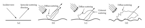
Figure 2.
Electromagnetic wave scattering from several different rough surfaces. (a) specular surface.; (b) slightly rough surface; (c) medium rough surface; (d) rough surface.
If the surface is relatively flat, the reflection is mainly specular from the First Fresnel zone, which is defined [44,45,46] by the ellipse of semi-axes:
In this equation is the wavelength, is the height of the receiver, and is the incidence angle. In addition to the coherent scattering, this also includes the diffuse scattering component from the glistening area.
Figure 1a shows the coherent scattering, while Figure 1b is the non-coherent scattering. From the comparison of these two subfigures, we can see that the coherent scattering under various polarizations is greater than that of non-coherent scattering. This is also consistent with the current CYGNSS data processing, where many researchers believe that the reflected energy is mainly coherent. However, the surface cannot be completely smooth, so that there is a certain degree of roughness, making the non-coherent scattering inevitable. Many simulations over the last year have visualized that topographic effects can produce dominantly incoherent data across Delay Doppler Maps [47,48]. Therefore, how to make good use of the non-coherent scattering energy and extract the bi-static radar cross-section from the receiver’s DDM waveform are vital for soil moisture retrieval.
3.3. Observation Geometry (Scattering Zenith Angle and Azimuth Angle)
The influence of the incidence angle for soil moisture inversion is rarely considered. Some researchers [31,33] only use a simple angle normalization, and [11] first attempted to include the incidence angle dependence in the soil moisture inversion. However, the authors in [11] employed a model that was limited to low incidence angles (θ < 30°). For GNSS-R, since the receiver can obtain data of a wide range of incidence angles (variable in terms of zenith and azimuth angles), this presents great advantages in front of other remote sensing techniques.
3.3.1. Scattering Zenith Angle
In this section, we simulate the specular and the bi-static scattering versus the scattering zenith angle under different polarizations. For this experiment we employ a soil moisture of 0.3 (surface permittivity ).
From Figure 3a it can be seen that except for the VR polarization, the specular scattering coefficient gradually decreases with the increase of the scattering angle. At a small incident angle, the LR polarization has the largest scattering, but at a larger incident angle, the HR polarization has the largest scattering. Note also that at the Brewster angle, there is a scattering groove at VR polarization, which will be shown in detail in Section 3.3.3. In Figure 3b, and the bi-static scattering occurs in the same plane. The scattering energy of LR polarization is larger than that of the other polarizations. We can see that as the scattering angle increases, the bi-static scattering first, increases, and then the scattering peak appears at . This effect is mainly at the incidence angle of 30°, when specular scattering occurs. In Figure 3c, , where the bi-static scattering occurs in a perpendicular plane. In this panel, we can see that the VR’s scattering is the smallest. As the scattering azimuth increases, the bi-static scattering decreases for the other polarizations. In Figure 3d-e, equals to 120° and 180°, respectively. When , the +45°R scattering is the lowest, and the scattered values of the other polarizations are very close. When , the difference between the scattering values of various polarizations is small.
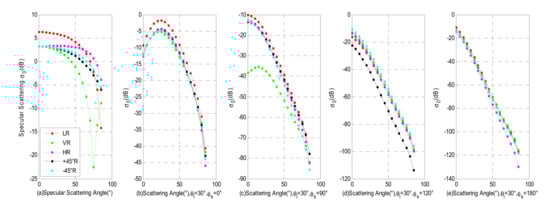
Figure 3.
Scattering properties of different polarization versus the specular/scattering angles: (a) Specular scattering; (b) bistatic scattering in one-plane ; (c) bistatic scattering in Perpendicular plane ; (d) bistatic scattering ; (e) bistatic scattering .
3.3.2. Scattering Azimuth Angles
The simulations of the scattering characteristics at different zenith angles are presented in Figure 3a–e. For the same observation target, the change of the observed azimuth angle will cause differences in the scattering characteristics. This is a dependence that cannot be ignored. The following analysis simulates the bi-static scattering properties of different polarizations versus the scattering azimuth angle. While the observation geometry is , the volumetric soil moisture is 0.3 (surface permittivity ).
In Figure 4 we can see that when the azimuth angle increases the scattering gradually decreases. At , in the specular plane, the scattering value is the largest. This is mainly due to the occurrence of specular scattering at this observation geometry.
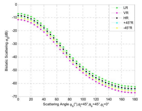
Figure 4.
Bi-static scattering of various polarizations versus scattering azimuth angle.
3.3.3. Brewster Angle
When a plane wave passes through the plane boundary between the lossless media, there is an angle at which full transmission occurs for vertical polarization. This angle is the Brewster angle , and full transmission does not occur for horizontal polarization [49].
In this equation, and are the permittivity of medium 1 and medium 2, respectively.
In Figure 3a, it can be seen that there is a scattering groove in the VR polarization, which is caused by the Brewster angle. This section analyzes the scattering grooves that appear in the VR polarization and the Brewster angles corresponding to different soil moisture cases.
In Figure 5 we can see that the Brewster angle generally occurs at larger angles, where the scattering of VR polarization disappears. When vegetation is abundant, a larger scattering at the VR polarization is possible. Therefore, the effect of vegetation can be effectively removed by the Brewster angle information at the VR polarization.
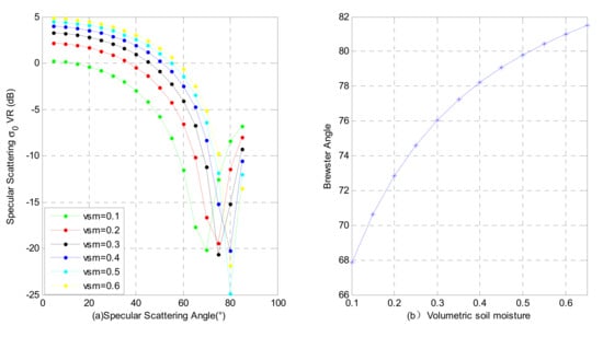
Figure 5.
VR scattering versus scattering angle and Brewster angle for different soil moisture cases. Figure (a) is the specular scattering at VR versus the scattering angle. While Figure (b) is the Brewster angle versus the volumetric soil moisture value.
3.4. Surface Roughness
The permittivity of the soil and the surface roughness are strongly coupled, and generally, it is difficult to distinguish which parameter influences the GNSS-R signal. Therefore, roughness is a very important factor that needs to be eliminated in soil moisture inversion. At present, the scientific community has had very little consideration on surface roughness, and only a few articles have conducted relevant research on surface roughness information [11,50]. These works employ the roughness coefficient to correct the reflectivity during the inversion process. This correction is highly dependent on the ancillary data [11,32]. For instance, the authors in [11] suggested that small variations in surface reflectivity will not influence the soil moisture retrieval below RMS roughness of ~0.2 m, while their tests carried out with ICESat-2 data showed the high sensitivity to high RMS roughness. In their experiment, the authors mentioned the high sensitivity of ICESat-2 to land surface microrelief, while SMAP RMS roughness showed relatively much lower values. This would indeed cause large differences in soil moisture estimation.
The surface roughness can be expressed by two parameters, namely the RMS height and the correlation length of the surface (CL). These two parameters define the surface roughness on the vertical and horizontal scales. In this section, we analyze the surface roughness effects (RMS and CL) with the LR polarization.
Figure 6a shows the specular scattering versus roughness (RMS and CL), where . At this observation geometry, as the roughness increases, the specular scattering energy decreases. In Figure 6b, the incident and scattering angles are in a plane, that is , but the incident angle is 30°, and the scattering angle is 50°. In this panel, the greater the roughness the greater the bi-static scattering. In Figure 6c, the azimuth angle is set to 120°, so that the scattering is not in a plane. In this panel, the roughness increases with the scattering energy, so that under different observation angles, the roughness has a greater influence on the bi-static scattering, which is a problem that needs to be accounted for in GNSS-R inversion. The elimination of the influence of roughness on soil moisture retrieval is a key issue for improving retrieval accuracy.
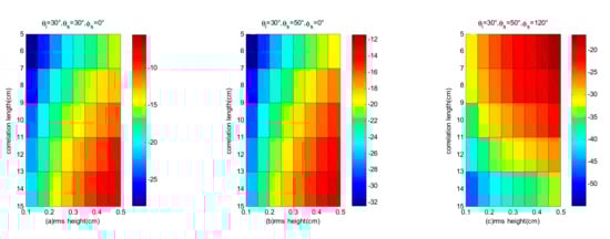
Figure 6.
The effect of surface roughness (RMS height and cl (correlation length)) on the bi-static scattering under different observation geometries. The polarization is LR. (a); (b) ; (c) .
3.5. Vegetation
In this section, we employ the first-order radiation-transfer equation to study the bi-static scattering characteristics when the ground is covered by vegetation (Aspen). The input of Aspen is shown in Table 1, and the permittivity of the trunks, branches, and soil are shown in Table 2. The scattering mechanisms include seven terms: D-G (direct ground), G-C-G (ground reflection and crown scattering and ground reflection), G-C (ground reflection and crown scattering), C-G (crown scattering and ground reflection) and D-C (direct crown scattering), T-G (trunk scattering and ground reflection), G-T (ground reflection and trunk scattering). The direct ground reflection term is D-G [36,37,38,41,42,43].

Table 1.
Input parameters of Aspen.
Table 2.
Input parameters of permittivity.
Our simulations are carried out for different incident angles and specular cones (Figure 7) where ki is the incident wave vector, ks the scattering wave vector, and x, y, and z are the local reference axes.
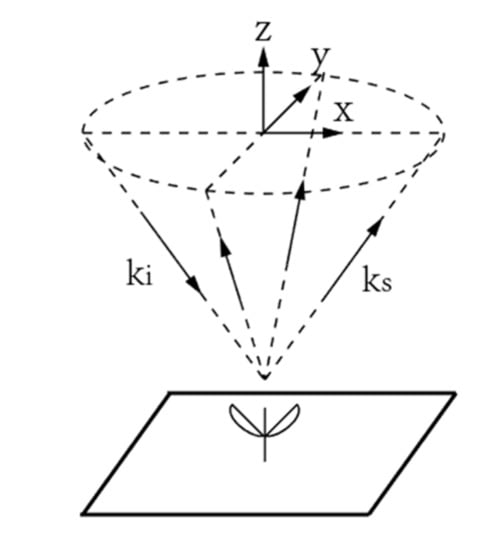
Figure 7.
Specular cone.
Figure 8 shows the scattering properties for incidence angles of 10°, 30°, and 80°. It can be seen that when the incidence angle increases, the contribution of the D-G term to the total scattering strongly varies. This dependence is mainly related to the scattering azimuth angle. When the incident angle has a small range (Figure 8a), the contribution of the D-G term is large, while the scattering azimuth angle is small. When the scattering azimuth angle increases, the contribution of the D-G term decreases. The G-T term strongly contributes to the total scattering energy. At a medium incidence angle (~30°, Figure 8b), the D-G term strongly contributes when the scattering azimuth is small. On the other hand, at a large scattering azimuth, the contribution of the D-G term can be ignored, and the G-T and T-G terms dominate the total scattering energy in the entire range of different scattering azimuth angles. At large incident angles (Figure 8c), the contribution of the D-C term increases, especially at medium and large scattering azimuth angles, while the influence of the D-G item can be completely ignored.
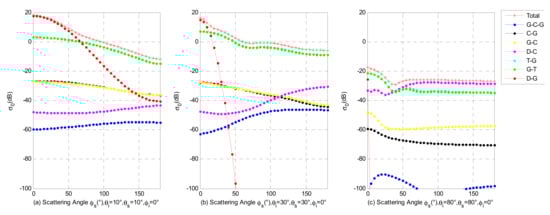
Figure 8.
Scattering characteristics at the specular cone for LR polarization. (a) ; (b) ; (c) .
In Figure 9 the specular scattering properties () show that while the specular angle increases the total scattering energy decreases. In the whole range of specular incident angles, the total scattered energy is dominated by the D-G term. The influence of the G-T term cannot be ignored, especially when the incident angle is large. Therefore, for GNSS-R, it is currently believed that the main energy received belongs to the specular scattering, so that the influence of vegetation on this geometry is relatively small. For a vegetation cover type such as that of Aspen (a representative forest canopy with vertical trunk layer), D-G terms mainly control the scattered energy. When the observation geometry changes, the influence of vegetation cannot be ignored, and affects the accuracy in soil moisture retrieval.
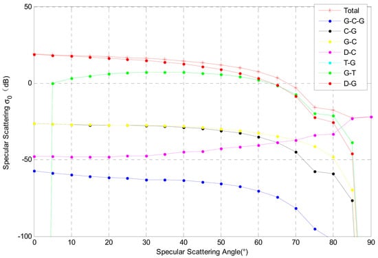
Figure 9.
The relationship of different scattering mechanisms with the incident angle during specular scattering.
Vegetation attenuates the incident GNSS signals and the reflected signals. The signals are scattered and reflected in the inner vegetation canopy layers, and some signals can even be absorbed. The scattering properties change for different observation geometries. Regarding the attenuation of vegetation for CYGNSS soil moisture retrieval, it is assumed that the attenuation due to VOD at different angles remains constant. This assumption was made during the inversion of soil moisture in [33]. However, the assumptions in the present research papers seem to be a little too simple. Here, the scattering properties of the Aspen cover type are presented using the vegetation radiative transfer equation model. From the simulations, we can see that the scattering properties for different scattering zenith angles and scattering azimuth angles are very different. Meanwhile, the scattering properties at various polarizations are very different. These simulations show that the vegetation attenuation cannot be assumed as a constant value for soil moisture retrieval. Moreover, the observation geometry and the polarization state are important aspects that should be also taken into consideration. Note the lack of scattering notches for the Aspen cover at any of the scattering angles, while there is an obvious scattering notch for bare soil. This means that for these angles, the ground surface scattering can be neglected, and the vegetation information can be retrieved from these angles, so that we can evaluate the vegetation properties during soil moisture retrieval process.
3.6. Effective Isotropic Radiated Power (EIRP)
Data calibration affects the accuracy of the acquired GNSS-R reflectivity data, which in turn affects the results of soil moisture retrieval. Currently, GNSS-R data calibration is an open issue, while EIRP is an important aspect for calibration. The EIRP is defined as the product of transmitted power and antenna gain pattern. As for the CYGNSS data calibration, EIRP is measured and calibrated by a ground-based GNSS power monitor system. DLR/GSOC’s measurements are used to verify the EIRP. These methods have a low cost, are highly robust, and can significantly reduce the PRN dependence while are used for CYGNSS calibration [51].
3.7. Radio Frequency Interference (RFI)
RFI refers to the interference phenomenon due to artificially emitted electromagnetic waves of similar frequency, which are received by the GNSS-R sensors. RFI can enter sensors through reflection, diffraction, atmospheric refraction, and scattering, and can cause an abnormal increase in the observation of reflected signals, as shown in Figure 10.
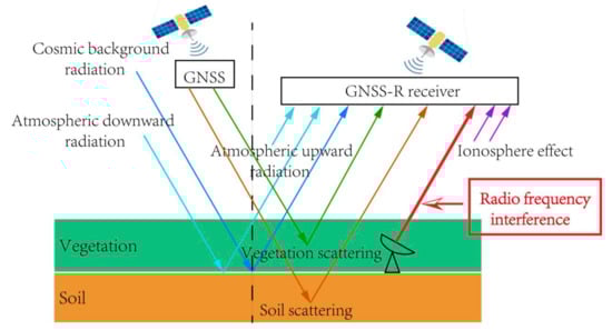
Figure 10.
RFI effects on the final GNSS-R power.
At present, there is a limited research on RFI for CYGNSS. Although is it stipulated by the International Telecommunication Union that the L-band can only be used for satellite Earth exploration services, in recent years, L-band satellites such as microwave radiometers have detected a large number of RFI signals. The L-band SMOS satellites have confirmed that RFI has a particular impact on data quality [52], and this has a serious impact on satellite observation accuracy and data inversion. RFI inevitably affects the quality of GNSS-R observation data, and to detect and suppress RFI is particularly important.
4. Conclusions
Based on the current research status of soil moisture using CYGNSS, this article summarizes and points out the problems in soil moisture retrieval, such as observation angles, coherent and non-coherent components, and dependence on ancillary data. Combined with the microwave bi-static full polarization scattering models, simulations of the coherent and non-coherent scattering characteristics at different polarizations and observation geometries have been analyzed. It is pointed out that the energy of coherent scattering is larger than that of non-coherent scattering. When the observation geometry changes, various polarizations have different scattering characteristics. VR polarization scattering grooves will appear at the Brewster angle, making full use of its information that can effectively remove the influence of roughness and vegetation effects. For specular scattering, the effect of vegetation is relatively small. D-G scattering dominates the total scattered energy, but the influence of vegetation on the total scattered energy cannot be ignored under changing the observation geometry. The surface roughness has different effects on the scattered energy under different observation geometries. Moreover, for data calibration, EIRP and RFI are two important aspects that cannot be ignored. These strongly affect the accuracy in soil moisture inversion. In general, several important development directions for GNSS-R soil moisture retrieval are suggested.
The first aspect is how to effectively extract coherent and non-coherent components from DDM observations in GNSS-R. Since at present it is an ambiguous aspect during the soil moisture retrieval, some researchers have pointed out that the noncoherent component will dominate the total DDMs, as we take the soil roughness into consideration.
The second aspect is to develop an inversion algorithm based on different incidence angles to expand the usable GNSS-R data for soil moisture inversion. At present, since the incidence angle information is not fully used during the retrieval, the ability of bistatic observation of various angles should be well developed.
Meanwhile, how to effectively remove the influence of vegetation and roughness in GNSS-R soil moisture inversion should also be investigated; these factors strongly affect the soil moisture retrieval accuracy.
Finally, other 2 important aspects for space-borne GNSS-R soil moisture retrieval are the calibration of EIRP and the suppression of RFI, so that GNSS-R data quality will improve.
Author Contributions
X.W., idea proposal, conceptualization, and original draft; W.M., figure plots; J.X., W.B., and S.J., suggestions and funding; A.C., tasks revisions and suggestions. All authors have read and agreed to the published version of the manuscript.
Funding
This research was funded by the National Natural Science Foundation of China (No. 42061057 and No. 41501384).
Data Availability Statement
Not applicable.
Acknowledgments
Special thanks are given to the anonymous reviewers who greatly helped to improve the quality of the manuscript.
Conflicts of Interest
The authors declare no conflict of interest.
Appendix A. Dielectric Constant Models
In this paper, we employ the random rough surface scattering models and first-order transfer equations model to do simulations and analysis [36,37]. One important input parameter for the scattering models is the dielectric constant model. For the soil dielectric constant model, we employ the mixed texture dielectric constant model [53,54]. For the vegetation dielectric constant model, we employ the Debye-Cole dual-dispersion model [55]. More details of the dielectric constant model are presented in Section 1. The developed scattering models are shown in Section 2.
Appendix A.1. Soil Dielectric Constant Models
In terms of electromagnetic characteristics, soil can be considered as the composition of four kinds of materials: air, solid particle, free water, and bound water. The final dielectric constant is the result of these four materials. The equation to get the mixed soil dielectric constant as follows [53,54]:
In this equation, is the dielectric constant, V is the volume for different components, is the shape factor, the subscripts s, a, fw, bw, and i indicate the components of solid material, air, free water, and bound water, respectively. The real part () and imaginary part () of the free water can be expressed as follows:
In these equations, is the electromagnetic wave frequency, is the permittivity of free space, effective conductivity is related to soil texture, and is the solid material density. is the high frequency of pure water dielectric constant and pure water static dielectric properties and the relaxation time of pure water are defined as:
where T is the soil temperature.
Appendix A.2. Vegetation Dielectric Constant
We employ the same model to calculate dielectric constants for all scatterers in vegetation canopy, such as leaves, branches, and trunks. [55] showed that the dielectric constant of vegetation can be calculated by the Debye-Cole dual dispersion model. The model consists on free water and bound water. According to the model, the dielectric constant of vegetation can be expressed as:
where,
in the above equations is environment temperature, and is the volume water content. If we know the dry material density of vegetation and the water content , then the volumetric water content can be expressed as:
Appendix B. Scattering Models
The 2 commonly used models are the backscattering model for active monostatic radar and the emissivity model for passive radiometer. However, for GNSS-R applications, the bistatic scattering model is necessary, since the GNSS constellation transmitter and the GNSS-R receiver form the typical bistatic radar system. Therefore, it is necessary to develop a new model in the bistatic form. Meanwhile, in order to overcome the ionospheric effect, the transmitted signals of GNSS are mainly right-hand circular polarization, while the commonly used microwave scattering models (both active and passive) use the linear form. Then, new models are necessary for the circular polarization systems. Moreover, with the development of the space-borne GNSS-R missions for land surface, the combination of circular polarization and linear polarization should be also analyzed, so that new models should be developed for various polarization combinations. The commonly used equations to develop these models can be obtained in the literature presented in this manuscript. Here, we illustrate the methods that are used in our model developments.
Appendix B.1. Polarization Coordinate System
There are basically 2 conventions for defining the polarization of an electromagnetic wave when considering the scattering from an object. The first convention defines the vertical and horizontal unit polarization vectors for the incident and scattered waves such that they are equal in the forward scatter direction, namely the FSA (Forward Scatter Alignment) convention (as shown in Figure A1) [36].

Figure A1.
Geometry for FSA convention.
Figure A1.
Geometry for FSA convention.

On the other side, the BSA (Back Scatter Alignment) convention defines the vertical and horizontal unit polarization vectors for the incident and scattered wave such that they are equal in the backscatter direction. The only difference between the BSA and FSA convention is that is replaced with . The BSA convention has been the standard used in the area of radar polarimetry. In order to obtain the various polarization combination using the wave synthesis technique, we perform this polarization coordinate systems conversion accordingly [36].
Appendix B.2. Angle Changes
For the vegetation part, we employ the first-order transfer equation model to get the vegetation scattering. As for the phase matrix and the extinction matrix, we change the angles to the bistatic form [37]. As for the extinction of the crown layer, we include the upward extinction matrix after the scattering is done by the trunk layer as well as the downward extinction matrices that are not scattered by the trunk layer . The extinction matrices in the trunk layer include 4 kinds: 2 upwards directions (one scattered by the trunk layer , and one not scatter by the crown layer ), and two downward directions (one scattered by the crown layer and one not scattered by the crown layer ). As for the calculation of the phase matrix, we include 4 kinds of observation angles combination: (1) the incident direction is , while the scattering direction is ; (2) the incident wave is , while the scattering direction is ; (3) the incident direction is , while the scattering direction is ; (4) the incident direction is , while the scattering direction is .
Appendix B.3. Wave Synthesis Technique
In order to get the various polarizations, we employ the wave synthesis technique [38]. The equation is as follows:
In this equation, Mm is the modified Mueller matrix, and Ym is the modified stokes vectors, where the upper subscript r and t indicate the polarization of transmitted and received signals. These depend on the variables of orientation ψ and ellipticity χ, respectively. The modified stokes vectors can be calculated as follows:
References
- Lekshmi, S.U.S.; Singh, D.N.; Baghini, M.S. A critical review of soil moisture measurement. Measurement 2014, 54, 92–105. [Google Scholar]
- Petropoulos, G.P.; Ireland, G.; Barrett, B. Surface soil moisture retrievals from remote sensing: Current status, products & future trends. Phys. Chem. Earth. Parts A B C 2015, 83–84, 36–56. [Google Scholar]
- KERR, Y.H. Soil moisture from space: Where are we? Hydrogeol. J. 2007, 15, 117. [Google Scholar] [CrossRef]
- Mccoll, K.A.; Alemohammad, S.H.; Akbar, R. The global distribution and dynamics of surface soil moisture. Nat. Geosci. 2017, 10, 100. [Google Scholar] [CrossRef]
- Malicki, M.A.; Skierucha, W.M. A manually controlled tdr soil moisture meter operating with 300 ps rise-time needle pulse. Irrig. Sci. 1989, 10, 153–163. [Google Scholar] [CrossRef]
- Ulaby, F.; Moore, R.; Fung, A. Microwave Remote Sensing: Active and Passive, 2-Radar Remote Sensing and Surface Scattering and Emission Theory; Artech House: Norwood, MA, USA, 1982. [Google Scholar]
- Entekhabi, D.; Njoku, E.G.; O’Neill, P.E. The soil moisture active passive (SMAP) mission. Proc. IEEE 2010, 98, 704–716. [Google Scholar] [CrossRef]
- Kerr, Y.H.; Waldteufel, P.; Richaume, P.; Wigneron, J.P.; Ferrazzoli, P.; Mahmoodi, A.; Al-Bitar, A.; Cabot, F.; Gruhier, C.; Juglea, S.E. The SMOS soil moisture retrieval algorithm. IEEE Trans. Geosci. Remote Sens. 2012, 50, 1384–1403. [Google Scholar] [CrossRef]
- Jackson, T.J., III. Measuring surface soil moisture using passive microwave remote sensing. Hydrol. Process. 1993, 7, 139–152. [Google Scholar] [CrossRef]
- Zavorotny, V.U.; Gleason, S. Tutorial on Remote Sensing Using GNSS Bistatic Radar of Opportunity. Geosci. Remote Sens. Mag. IEEE 2014, 2, 8–45. [Google Scholar] [CrossRef]
- Calabia, A.; Molina, I.; Jin, S. Soil Moisture Content from GNSS Reflectometry Using Dielectric Permittivity from Fresnel Reflection Coefficients. Remote Sens. 2020, 12, 122. [Google Scholar] [CrossRef]
- Edokossi, K.; Calabia, A.; Molina, I.; Jin, S. GNSS-Reflectometry and Remote Sensing of Soil Moisture: A Review of Measurement Techniques, Methods, and Applications. Remote Sens. 2020, 12, 614. [Google Scholar] [CrossRef]
- Masters, D.S. Surface Remote Sensing Applications of GNSS Bistatic Radar: Soil Moisture and Aircraft Altimetry. Ph.D. Thesis, University of Colorado, Boulder, CO, USA, 2004. [Google Scholar]
- Larson, K.M.; Small, E.E. Using GPS multipath to measure soil moisture fluctuations: Initial results. GPS Solut. 2008, 12, 173–177. [Google Scholar] [CrossRef]
- Chew, C.C.; Small, E.E. Effects of near-surface soil moisture on GPS SNR data: Development of a retrieval algorithm for soil moisture. IEEE Trans. Geosci. Remote Sens. 2013, 52, 537–543. [Google Scholar] [CrossRef]
- Rodriguez-Alvarez, N.; Bosch-Lluis, X. Soil Moisture Retrieval Using GNSS-R Techniques: Experimental Results Over a Bare Soil Field. IEEE Trans. Geosci. Remote Sens. 2009, 47, 3616–3624. [Google Scholar] [CrossRef]
- Rodriguez-Alvarez, N.; Camps, A. Land Geophysical Parameters Retrieval Using the Interference Pattern GNSS-R Technique. IEEE Trans. Geosci. Remote Sens. 2010, 49, 71–84. [Google Scholar] [CrossRef]
- Wan, W.; Bai, W. Initial results of China’s GNSS-R airborne campaign: Soil moisture retrievals. Sci. Bull. 2015, 60, 964–971. [Google Scholar] [CrossRef]
- Jia, Y.; Savi, P. Sensing soil moisture and vegetation using GNSS-R polarimetric measurement. Adv. Sp. Res. 2016, 59. [Google Scholar] [CrossRef]
- Gleason, S.; Adjrad, M. Sensing Ocean, Ice and Land Reflected Signals from Space: Results from the UK-DMC GPS Reflectometry Experiment. In Proceedings of the 18th International Technical Meeting of the Satellite Division of The Institute of Navigation, Long Beach, CA, USA, 13–16 September 2005. [Google Scholar]
- Unwin, M.; Jales, P.; Tye, J.; Gommenginger, C.; Foti, G.; Rosello, J. Spaceborne GNSS-Reflectometry on TechDemoSat-1: Early Mission Operations and Exploitation. IEEE J. Sel. Top. Appl. Earth Obs. Remote Sens. 2016, 9, 4525–4539. [Google Scholar] [CrossRef]
- Ruf, C.; Asharaf, S.S.; Balasubramaniam, R.; Gleason, S.; Lang, T.; McKague, D.; Twigg, D.; Waliser, D. In-Orbit Performance of the Constellation of CYGNSS Hurricane Satellites. Bull. Am. Meteorol. Soc. 2019. [Google Scholar] [CrossRef]
- Yu, K.; Li, Y.; Chang, X. Snow Depth Estimation Based on Combination of Pseudorange and Carrier Phase of GNSS Dual-Frequency Signals. IEEE Trans. Geosci. Remote Sens. 2019, 57, 1817–1828. [Google Scholar] [CrossRef]
- Jing, C.; Niu, X.; Duan, C.; Lu, F.; Yang, X. Sea surface wind speed retrieval from the first chinese gnss-r mission: Technique and preliminary results. Remote Sens. 2019, 11, 3013. [Google Scholar] [CrossRef]
- Sun, Y.; Liu, C.; Du, Q.; Wang, X.; Liu, C. Global Navigation Satellite System Occultation Sounder II (GNOS II). In Proceedings of the IGARSS IEEE International Geoscience & Remote Sensing Symposium, Fort Worth, TX, USA, 23–28 July 2017. [Google Scholar]
- Chew, C.; Shah, R. Demonstrating soil moisture remote sensing with observations from the UK TechDemoSat-1 satellite mission. Geophys. Res. Lett. 2016, 43. [Google Scholar] [CrossRef]
- Camps, A.; Park, H. Sensitivity of GNSS-R Spaceborne Observations to Soil Moisture and Vegetation. IEEE J. Sel. Top. Appl. Earth Obs. Remote Sens. 2016, 9, 4730–4742. [Google Scholar] [CrossRef]
- Chew, C.; Colliander, A.; Shah, R. The sensitivity of ground-reflected GNSS signals to near-surface soil moisture, as recorded by spaceborne receivers. In Proceedings of the IEEE International Symposium on Geoscience and Remote Sensing (IGARSS), Fort Worth, TX, USA, 23–28 July 2017. [Google Scholar]
- Camps, A.; Vall-llossera, M.; Park, H.; Portal, G.; Rossato, L. Sensitivity of tds-1 gnss-r reflectivity to soil moisture: Global and regional differences and impact of different spatial scales. Remote Sens. 2018, 10, 1856. [Google Scholar] [CrossRef]
- Chew, C.C.; Small, E.E. Soil moisture sensing using spaceborne GNSS reflections: Comparison of CYGNSS reflectivity to SMAP soil moisture. Geophys. Res. Lett. 2018, 45. [Google Scholar] [CrossRef]
- Kim, H.; Lakshmi, V. Use of Cyclone Global Navigation Satellite System (CyGNSS) Observations for Estimation of Soil Moisture. Geophys. Res. Lett. 2018, 45, 8272–8282. [Google Scholar] [CrossRef]
- Clarizia, M.P.; Pierdicca, N. Analysis of CYGNSS Data for Soil Moisture Retrieval. IEEE J. Sel. Top. Appl. Earth Obs. Remote Sens. 2019, 12, 2227–2235. [Google Scholar] [CrossRef]
- Al-Khaldi, M.M.; Johnson, J.T. Time-Series Retrieval of Soil Moisture Using CYGNSS. IEEE Trans. Geosci. Remote Sens. 2019, 1–10. [Google Scholar] [CrossRef]
- Yan, Q.; Huang, W. Pan-tropical soil moisture mapping based on a three-layer model from CYGNSS GNSS-R data. Remote Sens. Environ. 2020, 247, 111944. [Google Scholar] [CrossRef]
- Balakhder, A.M.; Al-Khaldi, M.M. On the Coherency of Ocean and Land Surface Specular Scattering for GNSS-R and Signals of Opportunity Systems. IEEE Trans. Geosci. Remote Sens. 2019, 99, 1–11. [Google Scholar] [CrossRef]
- Ulaby, F.T.; Sarabandi, K. Michigan microwave canopy scattering model. Int. J. Remote Sens. 1990, 11, 1223–1253. [Google Scholar] [CrossRef]
- Liang, P.; Pierce, L.E. Radiative transfer model for microwave bistatic scattering from forest canopies. IEEE Trans. Geosci. Remote Sens. 2005, 43, 2470–2483. [Google Scholar] [CrossRef]
- Ulaby, F.T.; Elachi, C. Radar Polarimetry for Geoscience Applications; Artech House: Norwood, MA, USA, 1990; p. 376. [Google Scholar]
- Zavorotny, V.; Masters, D. Seasonal polarimetric measurements of soil moisture using tower-based gps bistatic radar. In Proceedings of the 2003 IEEE International Geoscience and Remote Sensing Symposium—IGARSS, Toulouse, France, 21–25 July 2003. [Google Scholar]
- Alonso-Arroyo, A.; Camps, A. Improving the Accuracy of Soil Moisture Retrievals Using the Phase Difference of the Dual-Polarization GNSS-R Interference Patterns. IEEE Geosci. Remote Sens. Lett. 2014, 11, 2090–2094. [Google Scholar] [CrossRef]
- Wu, X.R.; Jin, S.G. Models and theoretical analysis of SoOP circular polarization bistatic scattering for random rough surfaces. Remote Sens. 2020, 12, 1506. [Google Scholar] [CrossRef]
- Wu, X.R.; Jin, S.G. A simulation study of GNSS-R polarimetric scattering from the bare soil surface based on the AIEM model. Adv. Meteorol. 2019, 2019, 3647473. [Google Scholar] [CrossRef]
- Wu, X.R.; Jin, S.G. GNSS-Reflectometry: Forest canopies polarization scattering properties and modeling. Adv. Sp. Res. 2014, 54, 863–870. [Google Scholar] [CrossRef]
- Caparrini, M. Using reflected GNSS Signals to Estimate Surface Features over Wide Ocean Areas; ESTEC Report no. 2003; 1998. [Google Scholar]
- Masters, D.; Axelrad, P.; Katzberg, S. Initial results of land-reflected GPS bistatic radar measurements in SMEX02. Remote Sens. Environ. 2004, 92, 507–520. [Google Scholar] [CrossRef]
- Katzberg, S.J.; Torres, O.; Grant, M.S.; Masters, D. Utilizing calibrated GPS reflected signals to estimate soil reflectivity and dielectric constant: Results from SMEX02. Remote Sens. Environ. 2006, 100, 17–28. [Google Scholar] [CrossRef]
- Dente, L.; Guerriero, L.; Comite, D.; Pierdicca, N. Space-Borne GNSS-R Signal Over a Complex Topography: Modeling and Validation. IEEE J. Sel. Top. Appl. Earth Obs. Remote Sens. 2020, 13, 1218–1233. [Google Scholar] [CrossRef]
- Guerriero, L.; Dente, L.; Comite, D.; Pierdicca, N. Simulations of Spaceborne GNSS-R Signal Over Mountain Areas. In Proceedings of the IGARSS 2019—2019 IEEE International Geoscience and Remote Sensing Symposium, Yokohama, Japan, 28 July–2 August 2019; pp. 8362–8365. [Google Scholar]
- Ulaby, F.T.; Mooore, R.K.; Fung, A.K. Microwave Remote Sensing, Volume I Microwave Remote Sensing Fundamentals and Radiometry; Artech House: Norwood, MA, USA, 1981. [Google Scholar]
- Stilla, D.; Zribi, M.; Pierdicca, N.; Baghdadi, N.; Huc, M. Desert Roughness Retrieval Using CYGNSS 375 GNSS-R Data. Remote Sens. 2020, 12, 743. [Google Scholar] [CrossRef]
- Wang, T.; Ruf, C.S. Design and Performance of a GPS Constellation Power Monitor System for Improved CYGNSS L1B Calibration. IEEE J. Sel. Top. Appl. Earth Obs. Remote Sens. 2019, 12, 26–36. [Google Scholar] [CrossRef]
- Zhao, T.J.; Shi, J.C.; Bindlish, R. Refinement of SMOS multiangular brightness temperature toward soil moisture retrieval and its analysis over reference targets. IEEE J. Sel. Top. Appl. Earth Obs. Remote Sens. 2015, 8, 589–603. [Google Scholar] [CrossRef]
- Hallikainen, M.T. Microwave dielectric behavior of wet soil-part 1: Empirical models and experimental observations. IEEE Trans. Geosci. Remote Sens. 1985, GE-23, 25–34. [Google Scholar] [CrossRef]
- Dobson, M.C. Microwave dielectric behavior of wet soil-Part II: Dielectric mixing models. IEEE Trans. Geosci. Remote Sens. 1985, GE-23, 35–46. [Google Scholar] [CrossRef]
- Ulaby, F.T.; El-Rayes, M.A. Microwave dielectric spectrum of vegetation, Part II: Dual-dispersion model. IEEE Trans. Geosci. Remote Sens. 1987, 25, 550–557. [Google Scholar] [CrossRef]


Publisher’s Note: MDPI stays neutral with regard to jurisdictional claims in published maps and institutional affiliations. |
© 2020 by the authors. Licensee MDPI, Basel, Switzerland. This article is an open access article distributed under the terms and conditions of the Creative Commons Attribution (CC BY) license (http://creativecommons.org/licenses/by/4.0/).