Seasonal Cropland Trends and Their Nexus with Agrometeorological Parameters in the Indus River Plain


Abstract
1. Introduction
2. Materials
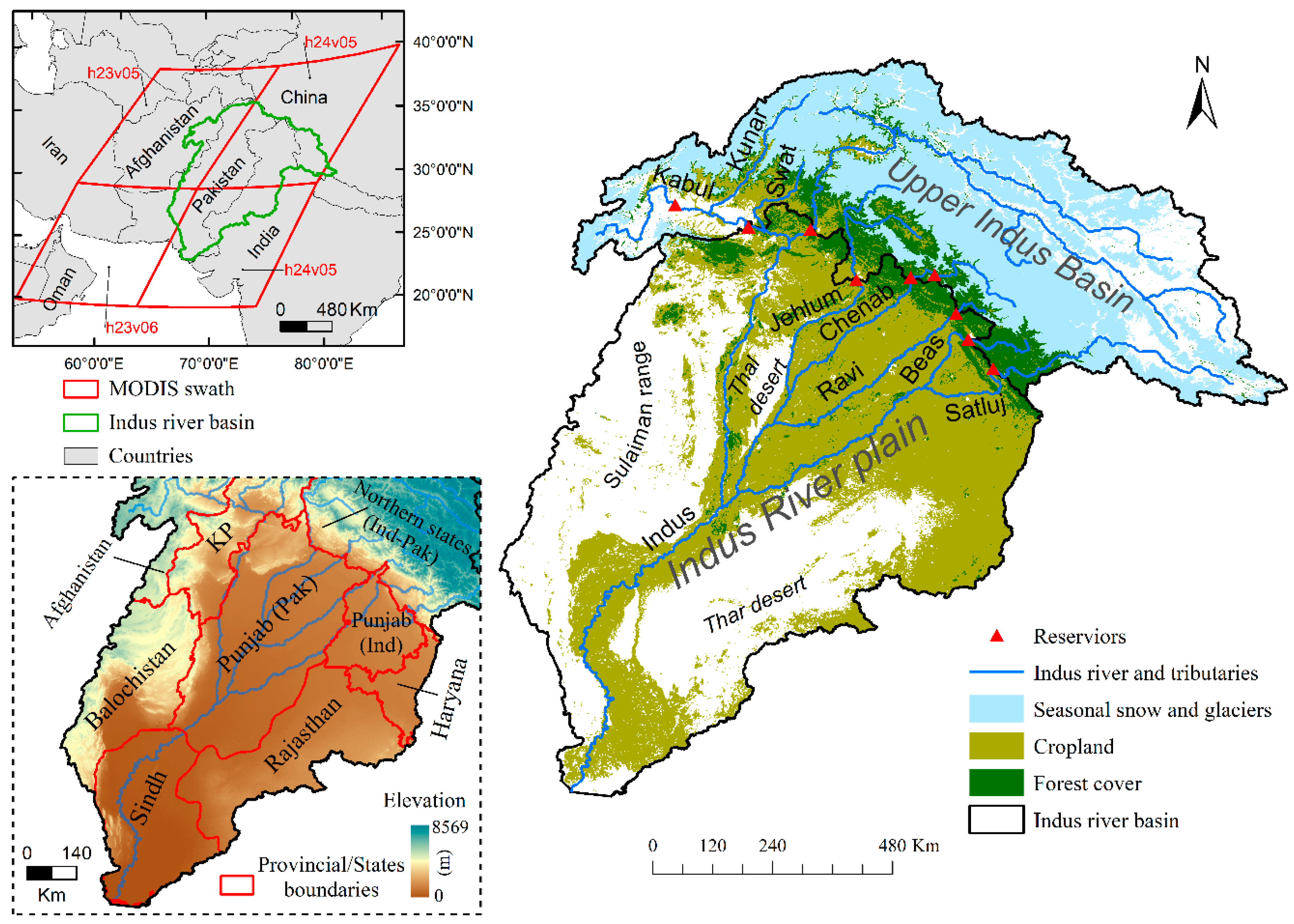
2.1. Study Area
2.2. Remote Sensing Data
2.3. Agrometeorological Data
3. Methods
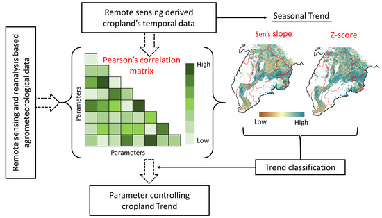
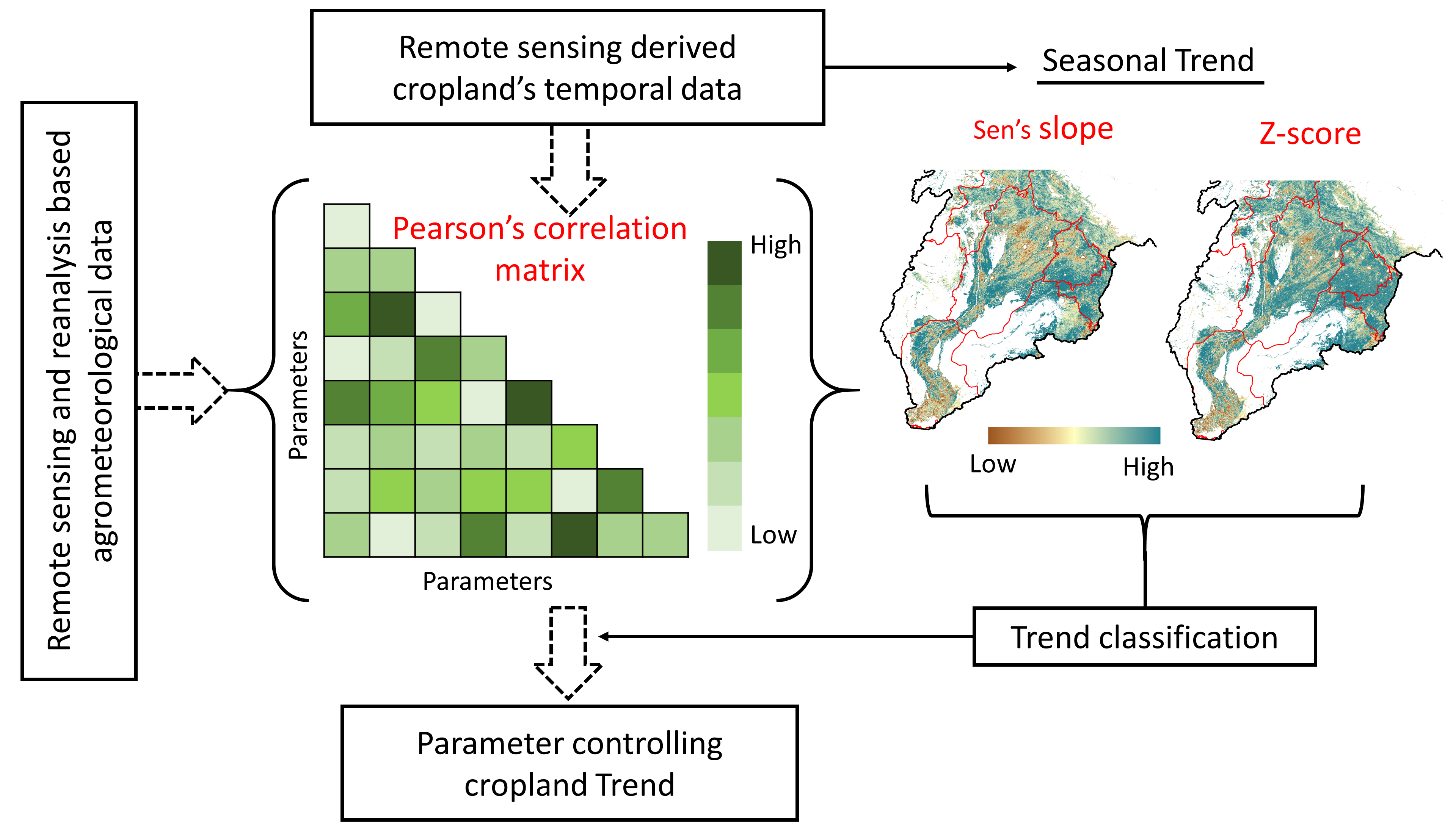
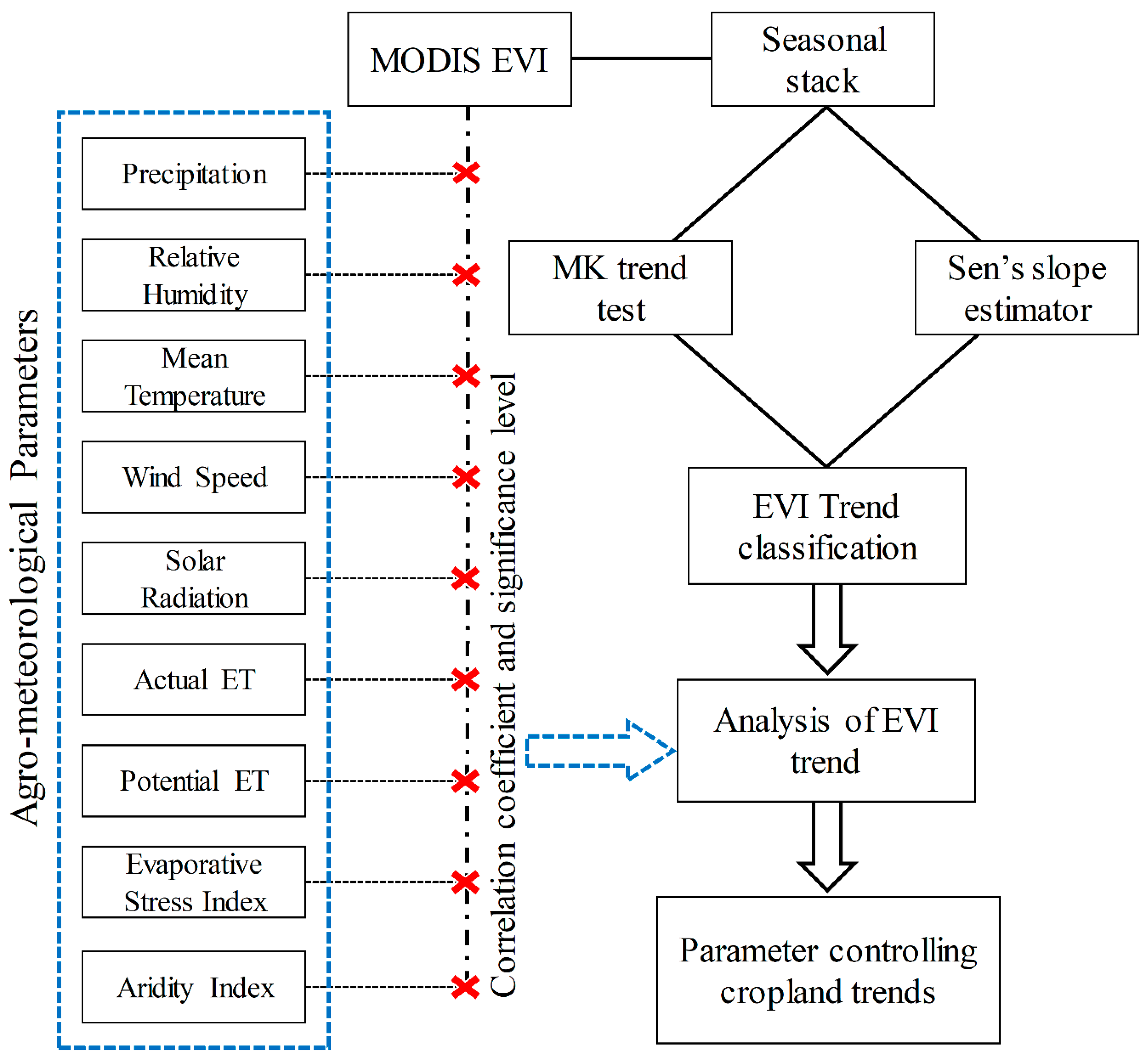
3.1. Overall Methodology
3.2. Trend Analysis
4. Results
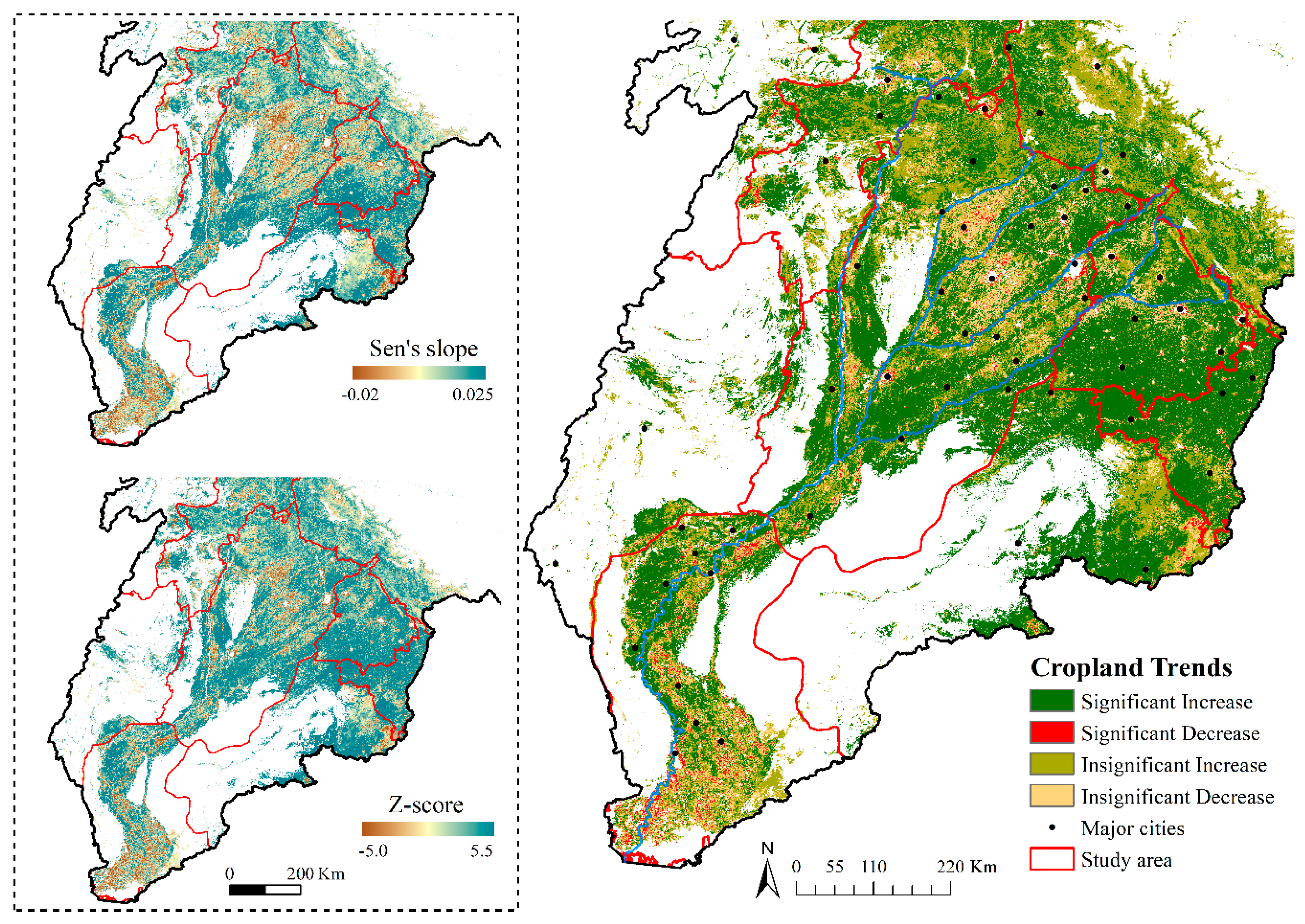
4.1. Spatial Variation of Seasonal Cropland Trends
4.1.1. Rabi Season
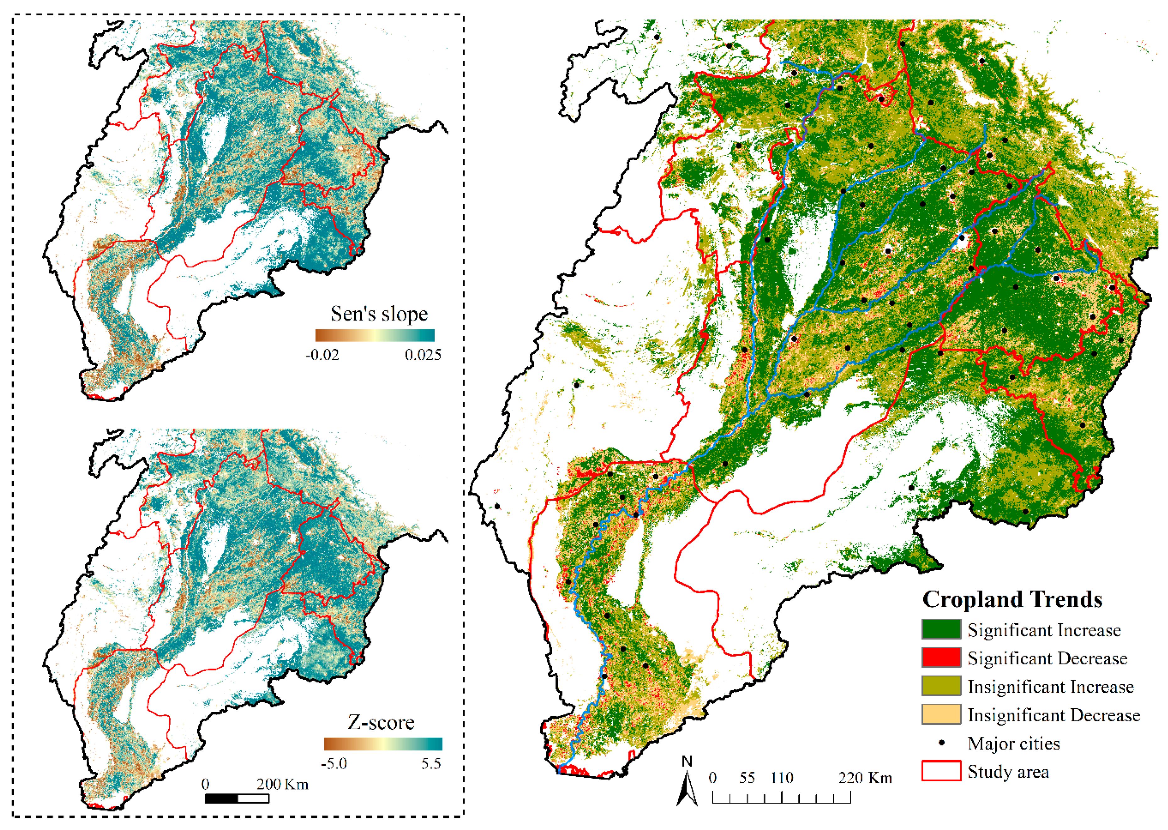
4.1.2. Kharif Season
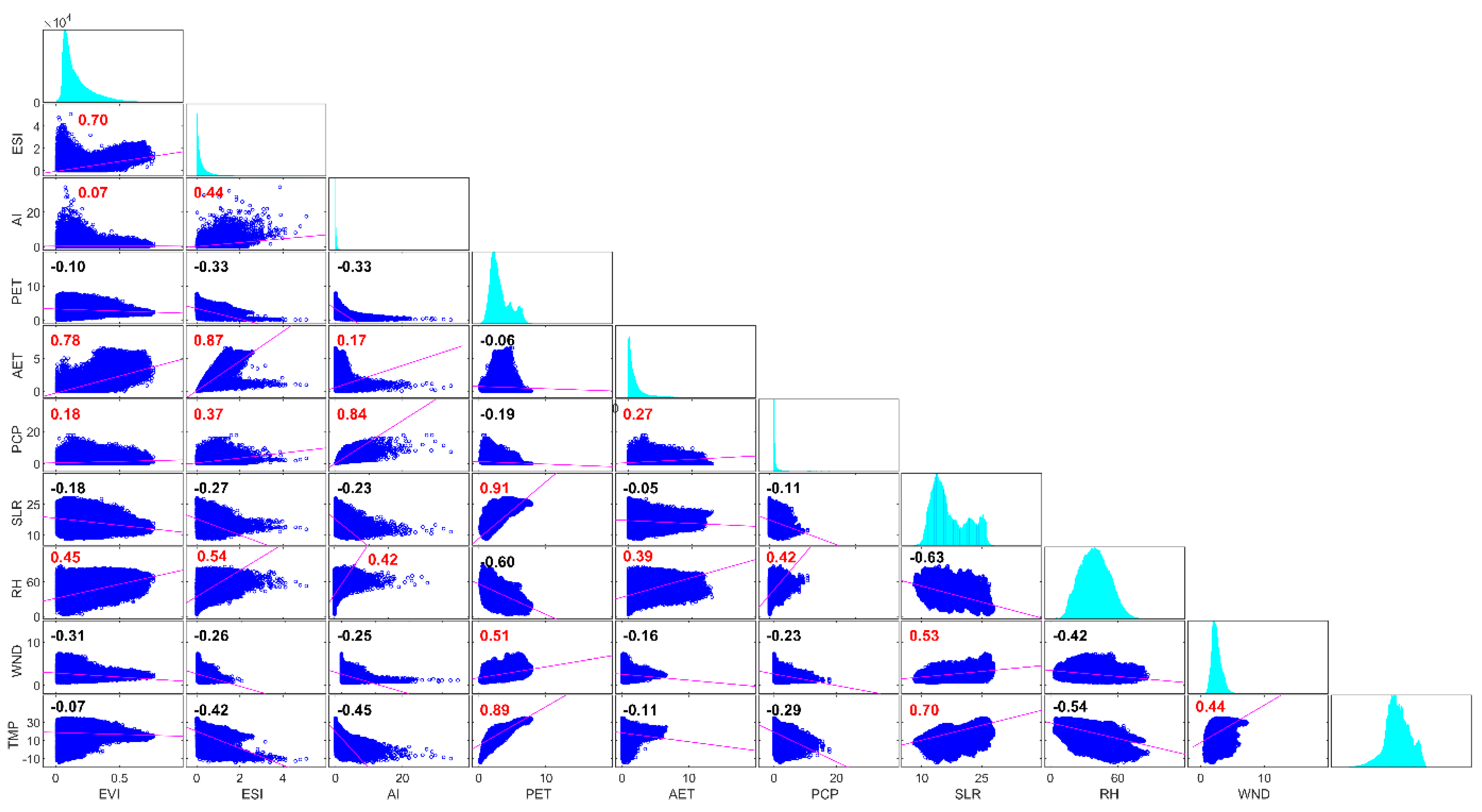
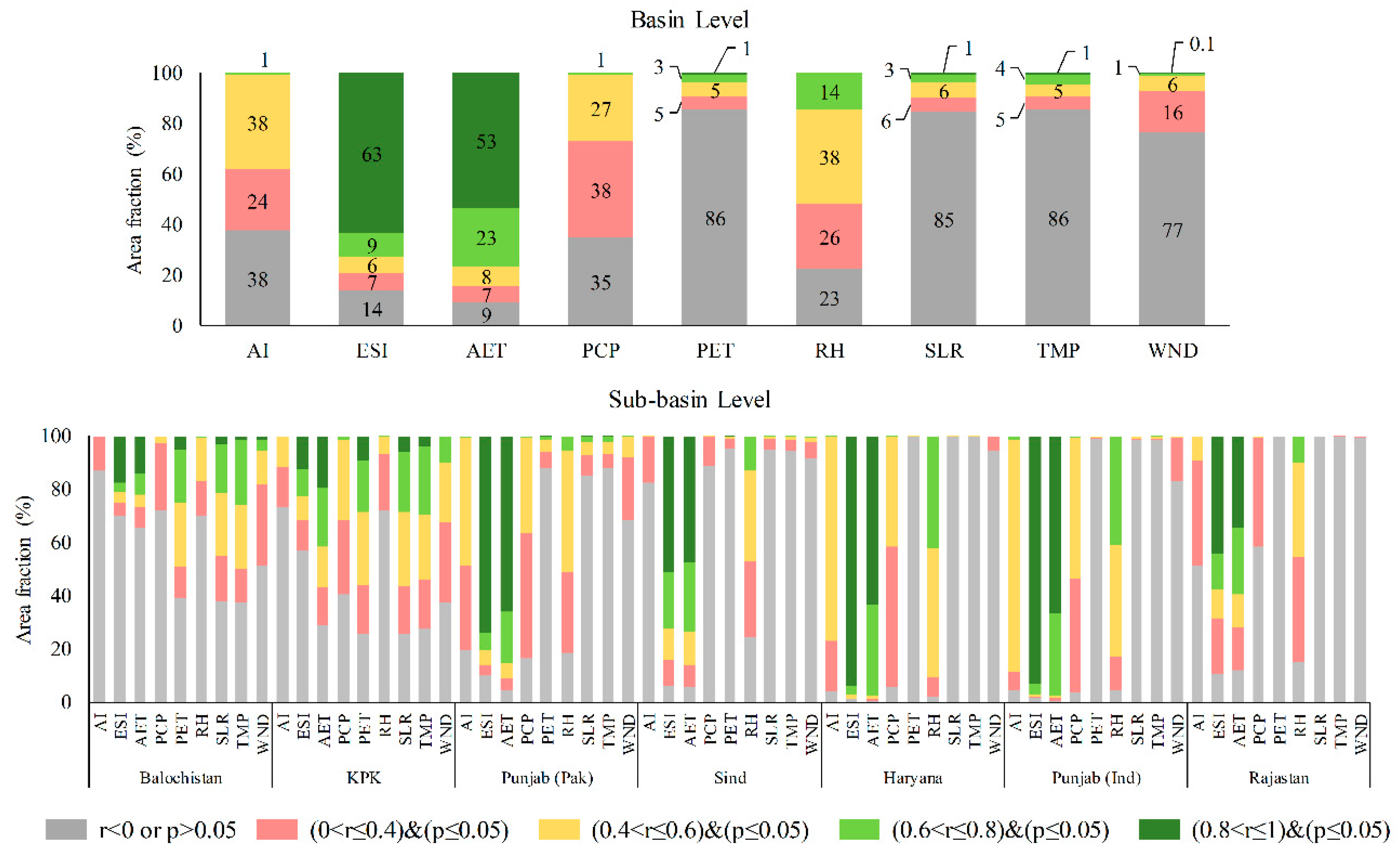
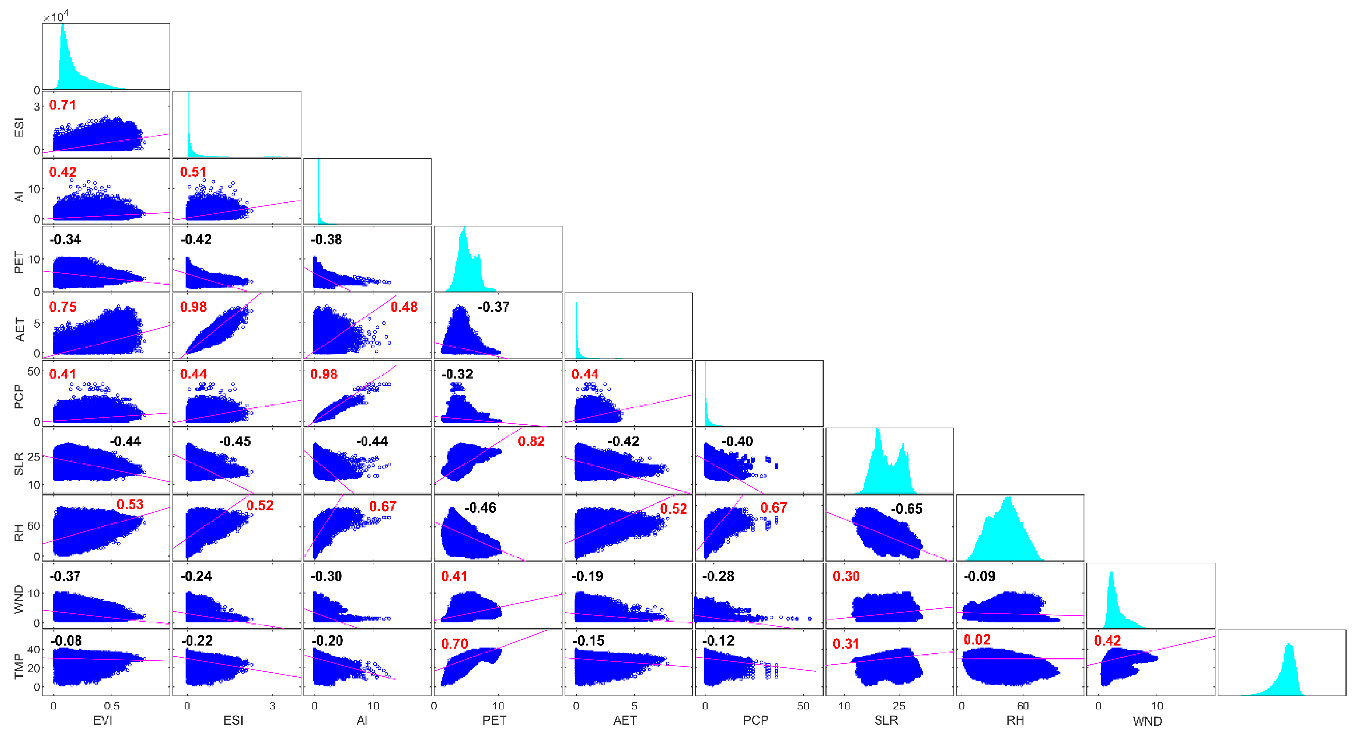
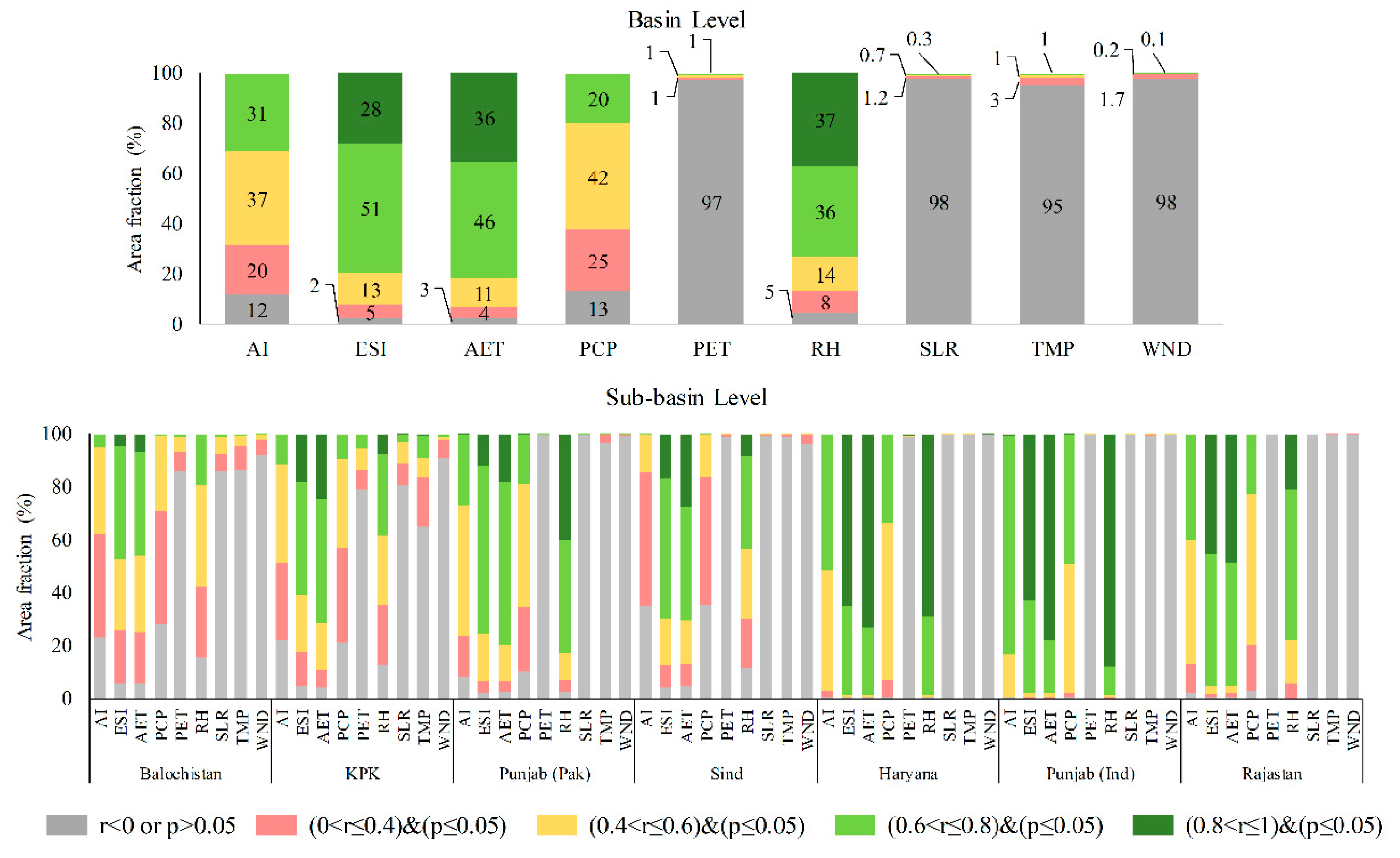
4.2. Nexus of Cropland and Agrometeorological Parameters
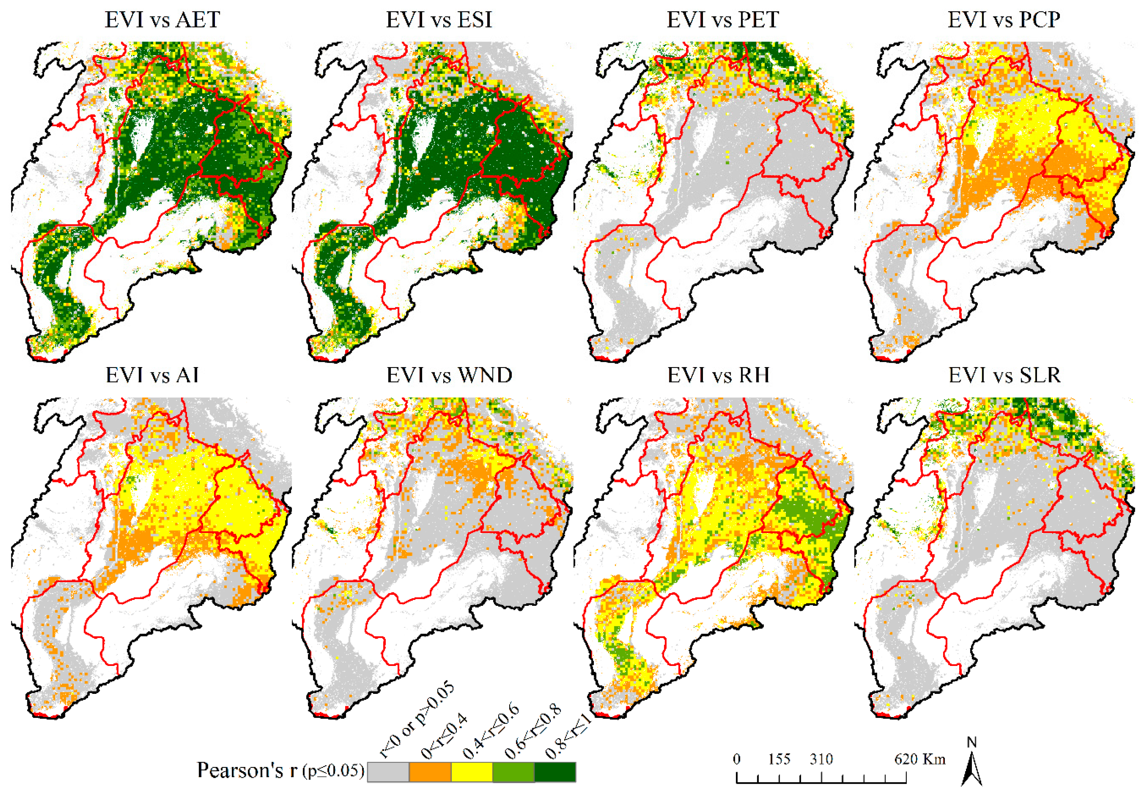
4.2.1. Rabi Season
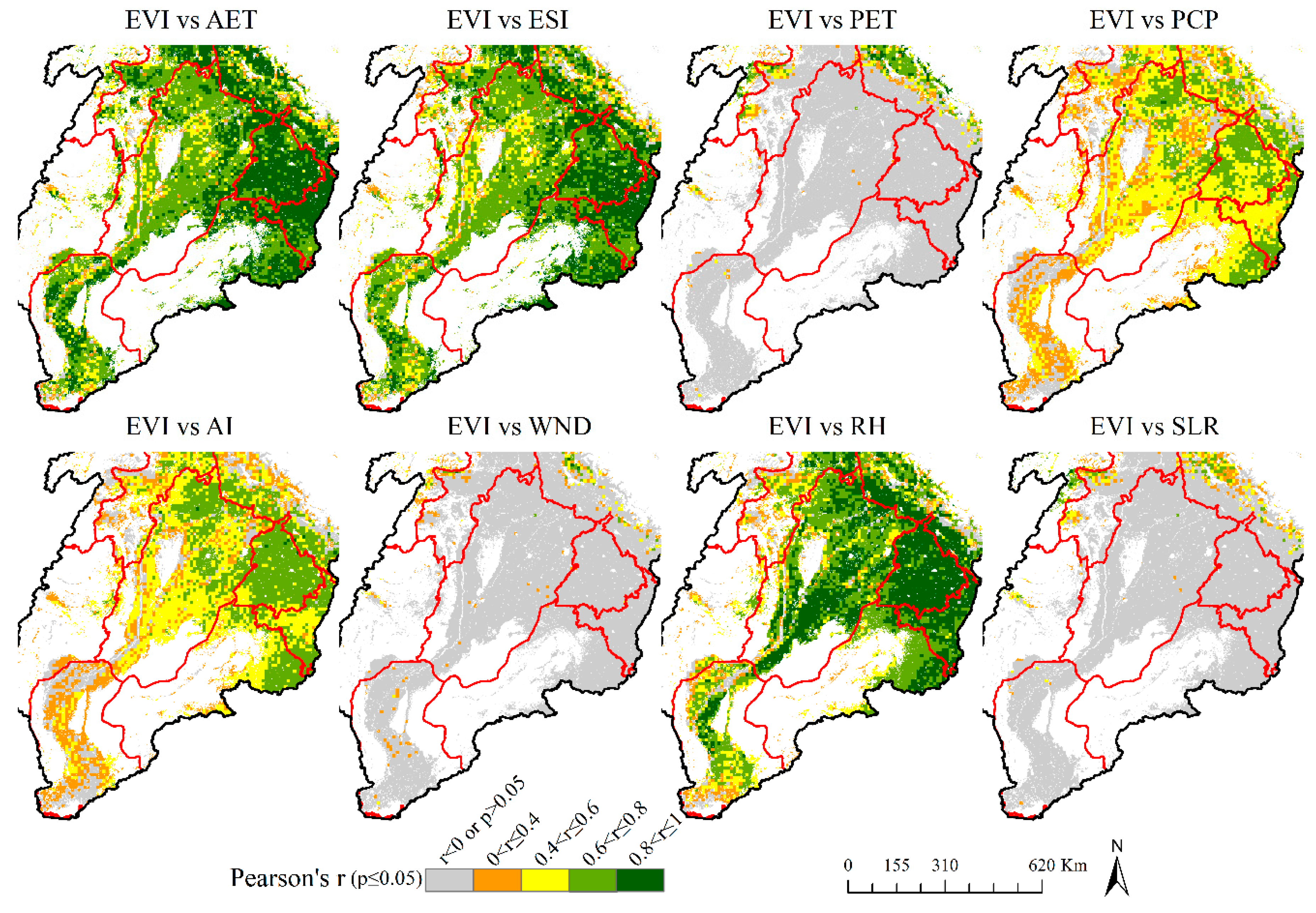
4.2.2. Kharif Season
5. Discussion
6. Conclusions
Author Contributions
Funding
Institutional Review Board Statement
Informed Consent Statement
Data Availability Statement
Conflicts of Interest
References
- Raza, A.; Razzaq, A.; Mehmood, S.S.; Zou, X.; Zhang, X.; Lv, Y.; Xu, J. Impact of climate change on crops adaptation and strategies to tackle its outcome: A review. Plants 2019, 8, 34. [Google Scholar] [CrossRef] [PubMed]
- Ray, D.K.; Gerber, J.S.; Macdonald, G.K.; West, P.C. Climate variation explains a third of global crop yield variability. Nat. Commun. 2015, 6, 5989. [Google Scholar] [CrossRef] [PubMed]
- Lobell, D.B.; Schlenker, W.; Costa-Roberts, J. Climate trends and global crop production since 1980. Science 2011, 333, 616–620. [Google Scholar] [CrossRef] [PubMed]
- Kukal, M.S.; Irmak, S. Climate-Driven Crop Yield and Yield Variability and Climate Change Impacts on the U.S. Great Plains Agricultural Production. Sci. Rep. 2018, 8, 1–18. [Google Scholar] [CrossRef] [PubMed]
- Zhang, Y.; Zhang, C.; Wang, Z.; Chen, Y.; Gang, C.; An, R.; Li, J. Vegetation dynamics and its driving forces from climate change and human activities in the Three-River Source Region, China from 1982 to 2012. Sci. Total Environ. 2016, 563, 210–220. [Google Scholar] [CrossRef]
- Zhang, Y.; Song, C.; Band, L.E.; Sun, G.; Li, J. Reanalysis of global terrestrial vegetation trends from MODIS products: Browning or greening? Remote Sens. Environ. 2017, 191, 145–155. [Google Scholar] [CrossRef]
- Pan, N.; Feng, X.; Fu, B.; Wang, S.; Ji, F.; Pan, S. Increasing global vegetation browning hidden in overall vegetation greening: Insights from time-varying trends. Remote Sens. Environ. 2018, 214, 59–72. [Google Scholar] [CrossRef]
- Qu, S.; Wang, L.; Lin, A.; Zhu, H.; Yuan, M. What drives the vegetation restoration in Yangtze River basin, China: Climate change or anthropogenic factors? Ecol. Indic. 2018, 90, 438–450. [Google Scholar] [CrossRef]
- Qu, S.; Wang, L.; Lin, A.; Yu, D.; Yuan, M.; Li, C. Distinguishing the impacts of climate change and anthropogenic factors on vegetation dynamics in the Yangtze River Basin, China. Ecol. Indic. 2020, 108, 105724. [Google Scholar] [CrossRef]
- Wang, F.; Liang, W.; Fu, B.; Jin, Z.; Yan, J.; Zhang, W.; Fu, S.; Yan, N. Changes of cropland evapotranspiration and its driving factors on the loess plateau of China. Sci. Total Environ. 2020, 728, 138582. [Google Scholar] [CrossRef]
- Tang, J.; Di, L. Past and future trajectories of farmland loss due to rapid urbanization using Landsat imagery and the Markov-CA model: A case study of Delhi, India. Remote Sens. 2019, 11, 180. [Google Scholar] [CrossRef]
- Gumma, M.K.; Mohammad, I.; Nedumaran, S.; Whitbread, A.; Lagerkvist, C.J. Urban sprawl and adverse impacts on agricultural land: A case study on Hyderabad, India. Remote Sens. 2017, 9, 1136. [Google Scholar] [CrossRef]
- Xu, Y.; Yu, L.; Zhao, F.R.; Cai, X.; Zhao, J.; Lu, H.; Gong, P. Tracking annual cropland changes from 1984 to 2016 using time-series Landsat images with a change-detection and post-classification approach: Experiments from three sites in Africa. Remote Sens. Environ. 2018, 218, 13–31. [Google Scholar] [CrossRef]
- Liu, F.; Zhang, Z.; Zhao, X.; Wang, X.; Zuo, L.; Wen, Q.; Yi, L.; Xu, J.; Hu, S.; Liu, B. Chinese cropland losses due to urban expansion in the past four decades. Sci. Total Environ. 2019, 650, 847–857. [Google Scholar] [CrossRef]
- Fassnacht, F.E.; Schiller, C.; Kattenborn, T.; Zhao, X.; Qu, J. A Landsat-based vegetation trend product of the Tibetan Plateau for the time-period 1990–2018. Sci. Data 2019, 6, 1–11. [Google Scholar] [CrossRef]
- Liu, Y.; Li, L.; Chen, X.; Zhang, R.; Yang, J. Temporal-spatial variations and influencing factors of vegetation cover in Xinjiang from 1982 to 2013 based on GIMMS-NDVI3g. Glob. Planet. Chang. 2018, 169, 145–155. [Google Scholar] [CrossRef]
- Lamchin, M.; Lee, W.K.; Jeon, S.W.; Wang, S.W.; Lim, C.H.; Song, C.; Sung, M. Long-term trend and correlation between vegetation greenness and climate variables in Asia based on satellite data. Sci. Total Environ. 2018, 618, 1089–1095. [Google Scholar] [CrossRef]
- Zhao, Q.; Ma, X.; Liang, L.; Yao, W. Spatial-temporal variation characteristics of multiple meteorological variables and vegetation over the loess plateau region. Appl. Sci. 2020, 10, 1000. [Google Scholar] [CrossRef]
- Zhang, Y.; Wang, X.; Li, C.; Cai, Y.; Yang, Z.; Yi, Y. NDVI dynamics under changing meteorological factors in a shallow lake in future metropolitan, semiarid area in North China. Sci. Rep. 2018, 8, 1–13. [Google Scholar] [CrossRef]
- Running, S.; Mu, Q.; Zhao, M.; Moreno, A. MODIS Global Terrestrial Evapotranspiration (ET) Product (NASA MOD16A2/A3) NASA Earth Observing System MODIS Land Algorithm; NASA: Washington, DC, USA, 2017.
- Hersbach, H.; Bell, B.; Berrisford, P.; Hirahara, S.; Horányi, A.; Muñoz-Sabater, J.; Nicolas, J.; Peubey, C.; Radu, R.; Schepers, D.; et al. The ERA5 global reanalysis. Q. J. R. Meteorol. Soc. 2020, 146, 1999–2049. [Google Scholar] [CrossRef]
- Urraca, R.; Huld, T.; Gracia-Amillo, A.; Martinez-de-Pison, F.J.; Kaspar, F.; Sanz-Garcia, A. Evaluation of global horizontal irradiance estimates from ERA5 and COSMO-REA6 reanalyses using ground and satellite-based data. Sol. Energy 2018, 164, 339–354. [Google Scholar] [CrossRef]
- Nogueira, M. Inter-comparison of ERA-5, ERA-interim and GPCP rainfall over the last 40 years: Process-based analysis of systematic and random differences. J. Hydrol. 2020, 583, 124632. [Google Scholar] [CrossRef]
- Tarek, M.; Brissette, F.P.; Arsenault, R. Evaluation of the ERA5 reanalysis as a potential reference dataset for hydrological modelling over North America. Hydrol. Earth Syst. Sci. 2020, 24, 2527–2544. [Google Scholar] [CrossRef]
- Belmonte Rivas, M.; Stoffelen, A. Characterizing ERA-Interim and ERA5 surface wind biases using ASCAT. Ocean Sci. 2019, 15, 831–852. [Google Scholar] [CrossRef]
- Hargreaves, G.H. Moisture availability and crop production. Trans. ASAE 1975, 18, 0980–0984. [Google Scholar] [CrossRef]
- Barrow, C.J. World atlas of desertification (United nations environment programme), edited by N. Middleton and D. S. G. Thomas. Edward Arnold, London. Land Degrad. Dev. 1992, 3, 249. [Google Scholar] [CrossRef]
- Allen, R.G.; Pereira, L.S.; Raes, D.; Smith, M. Crop Evapotranspiration—Guidelines for Computing Crop Water Requirements—FAO Irrigation and Drainage Paper 56; FAO: Rome, Italy, 1998. [Google Scholar]
- Kendall, M.G. Rank Correlation Methods. In Biometrika; Oxford University Press: Oxford, UK, 1957; p. 298. [Google Scholar]
- Mann, H.B. Nonparametric Tests Against Trend. Econometrica 1945, 13, 245–259. [Google Scholar] [CrossRef]
- Kisi, O.; Ay, M. Comparison of Mann-Kendall and innovative trend method for water quality parameters of the Kizilirmak River, Turkey. J. Hydrol. 2014, 513, 362–375. [Google Scholar] [CrossRef]
- Sen, P.K. Estimates of the Regression Coefficient Based on Kendall’s Tau. J. Am. Stat. Assoc. 1968, 63, 1379–1389. [Google Scholar] [CrossRef]
- Sarmah, S.; Jia, G.; Zhang, A.; Singha, M. Assessing seasonal trends and variability of vegetation growth from NDVI3G, MODIS NDVI and EVI over South Asia. Remote Sens. Lett. 2018, 9, 1195–1204. [Google Scholar] [CrossRef]
- Gao, X.; Liang, S.; He, B. Detected global agricultural greening from satellite data. Agric. For. Meteorol. 2019, 276, 107652. [Google Scholar] [CrossRef]
- Nabil, M.; Zhang, M.; Bofana, J.; Wu, B.; Stein, A.; Dong, T.; Zeng, H.; Shang, J. Assessing factors impacting the spatial discrepancy of remote sensing based cropland products: A case study in Africa. Int. J. Appl. Earth Obs. Geoinf. 2020, 85, 102010. [Google Scholar] [CrossRef]
- Javadian, M.; Behrangi, A.; Smith, W.K.; Fisher, J.B. Global trends in evapotranspiration dominated by increases across large cropland regions. Remote Sens. 2020, 12, 1221. [Google Scholar] [CrossRef]
- Anderson, M.C.; Zolin, C.A.; Sentelhas, P.C.; Hain, C.R.; Semmens, K.; Tugrul Yilmaz, M.; Gao, F.; Otkin, J.A.; Tetrault, R. The Evaporative Stress Index as an indicator of agricultural drought in Brazil: An assessment based on crop yield impacts. Remote Sens. Environ. 2016, 174, 82–99. [Google Scholar] [CrossRef]
- Krakauer, N.Y.; Cook, B.I.; Puma, M.J. Effect of irrigation on humid heat extremes. Environ. Res. Lett. 2020, 15, 094010. [Google Scholar] [CrossRef]
- Kimura, R. Global detection of aridification or increasing wetness in arid regions from 2001 to 2013. Nat. Hazards 2020, 103, 2261–2276. [Google Scholar] [CrossRef]
- Dimri, A.P.; Kumar, D.; Chopra, S.; Choudhary, A. Indus River Basin: Future climate and water budget. Int. J. Climatol. 2019, 39, 395–406. [Google Scholar] [CrossRef]
- Adnan, M.; Nabi, G.; Saleem Poomee, M.; Ashraf, A. Snowmelt runoff prediction under changing climate in the Himalayan cryosphere: A case of Gilgit River Basin. Geosci. Front. 2017, 8, 941–949. [Google Scholar] [CrossRef]
- Usman, M.; Abbas, A.; Saqib, Z.A. Conjunctive use of water and its management for enhanced productivity of major crops across tertiary canal irrigation system of indus basin in Pakistan. Pak. J. Agric. Sci. 2016, 53, 257–264. [Google Scholar] [CrossRef]


| Sub-Basin/Trend Class | Increase (p < 0.05) | Decrease (p < 0.05) | Increase (p > 0.05) | Decrease (p > 0.05) |
|---|---|---|---|---|
| Balochistan | 56.75 | 0.79 | 8.36 | 34.10 |
| KP | 48.24 | 1.72 | 12.45 | 37.59 |
| Punjab (Pak) | 55.54 | 2.09 | 16.79 | 25.58 |
| Sindh | 39.87 | 6.67 | 23.01 | 30.44 |
| Haryana | 76.82 | 0.90 | 6.80 | 15.48 |
| Punjab (Ind) | 71.03 | 0.98 | 13.15 | 14.85 |
| Rajasthan | 67.28 | 1.07 | 6.43 | 25.21 |
| Sub-Basin/Trend Class | Increase (p < 0.05) | Decrease (p < 0.05) | Increase (p > 0.05) | Decrease (p > 0.05) |
|---|---|---|---|---|
| Balochistan | 26.95 | 5.33 | 44.29 | 23.44 |
| KP | 47.35 | 1.04 | 42.30 | 9.31 |
| Punjab (Pak) | 52.46 | 1.88 | 34.67 | 10.99 |
| Sindh | 27.04 | 6.26 | 36.20 | 30.50 |
| Haryana | 53.54 | 0.98 | 29.65 | 15.84 |
| Punjab (Ind) | 68.15 | 1.11 | 15.46 | 15.28 |
| Rajasthan | 61.89 | 0.14 | 35.96 | 2.01 |
| No. | Nexus Level | R-Value | p-Value |
|---|---|---|---|
| 1 | Strong | >0.8 to 1 | ≤0.05 |
| 2 | Relatively Strong | >0.6 to 0.8 | ≤0.05 |
| 3 | Moderate | >0.4 to 0.6 | ≤0.05 |
| 4 | Weak | >0 to 0.4 | ≤0.05 |
| 5 | No Nexus | <0 | >0.05 |
Publisher’s Note: MDPI stays neutral with regard to jurisdictional claims in published maps and institutional affiliations. |
© 2020 by the authors. Licensee MDPI, Basel, Switzerland. This article is an open access article distributed under the terms and conditions of the Creative Commons Attribution (CC BY) license (http://creativecommons.org/licenses/by/4.0/).
Share and Cite
Zhou, Q.; Ismaeel, A. Seasonal Cropland Trends and Their Nexus with Agrometeorological Parameters in the Indus River Plain. Remote Sens. 2021, 13, 41. https://doi.org/10.3390/rs13010041
Zhou Q, Ismaeel A. Seasonal Cropland Trends and Their Nexus with Agrometeorological Parameters in the Indus River Plain. Remote Sensing. 2021; 13(1):41. https://doi.org/10.3390/rs13010041
Chicago/Turabian StyleZhou, Qiming, and Ali Ismaeel. 2021. "Seasonal Cropland Trends and Their Nexus with Agrometeorological Parameters in the Indus River Plain" Remote Sensing 13, no. 1: 41. https://doi.org/10.3390/rs13010041
APA StyleZhou, Q., & Ismaeel, A. (2021). Seasonal Cropland Trends and Their Nexus with Agrometeorological Parameters in the Indus River Plain. Remote Sensing, 13(1), 41. https://doi.org/10.3390/rs13010041