Instance Segmentation for Large, Multi-Channel Remote Sensing Imagery Using Mask-RCNN and a Mosaicking Approach

 ,
,  ,
,  , , ,
, , ,  , , and
Abstract
1. Introduction
Related Works on Center Pivot Detection
2. Materials and Methods
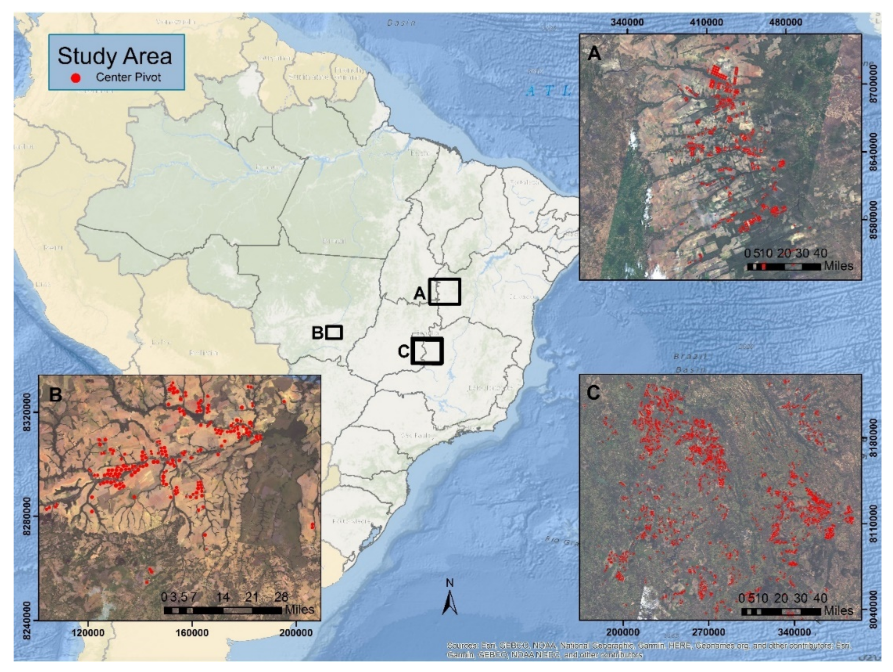
2.1. Dataset and Study Areas
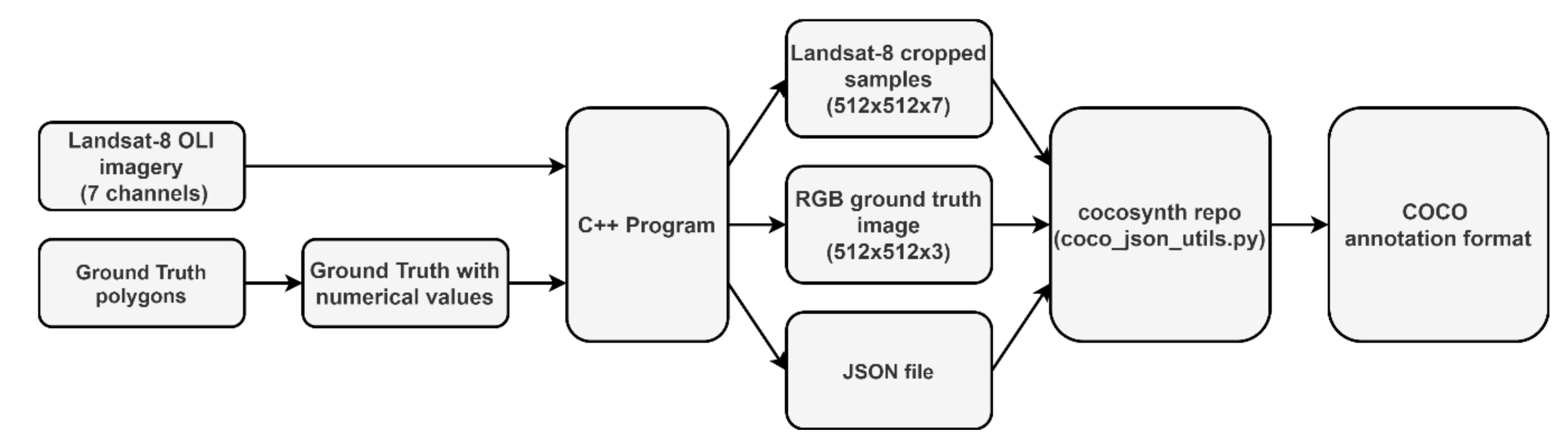
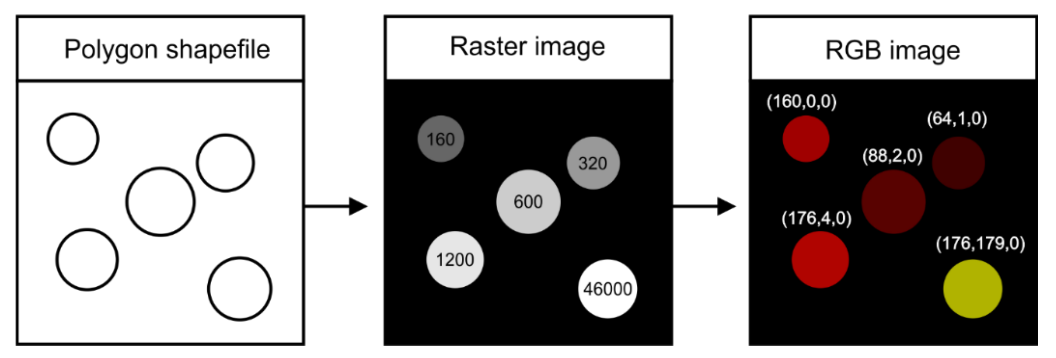
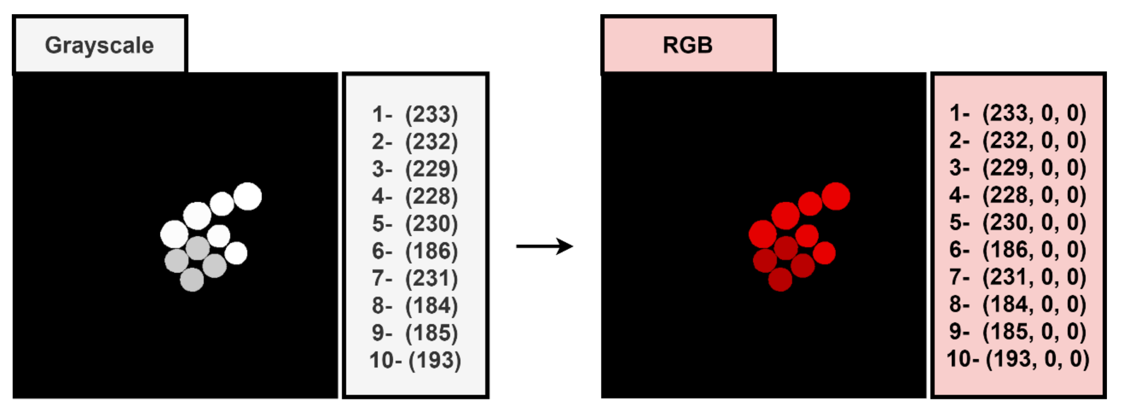
2.2. COCO Annotation Format
2.3. Data Split
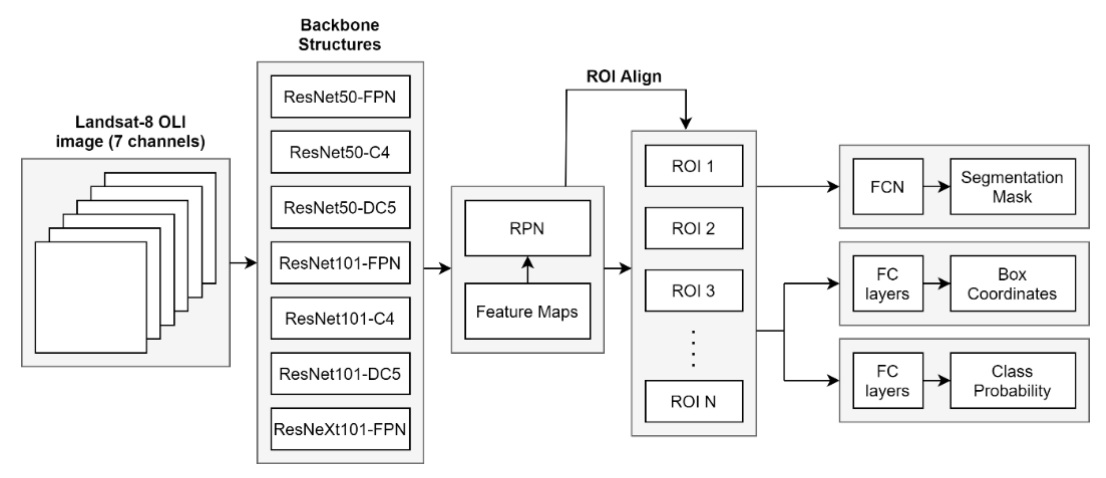
2.4. Mask R-CNN
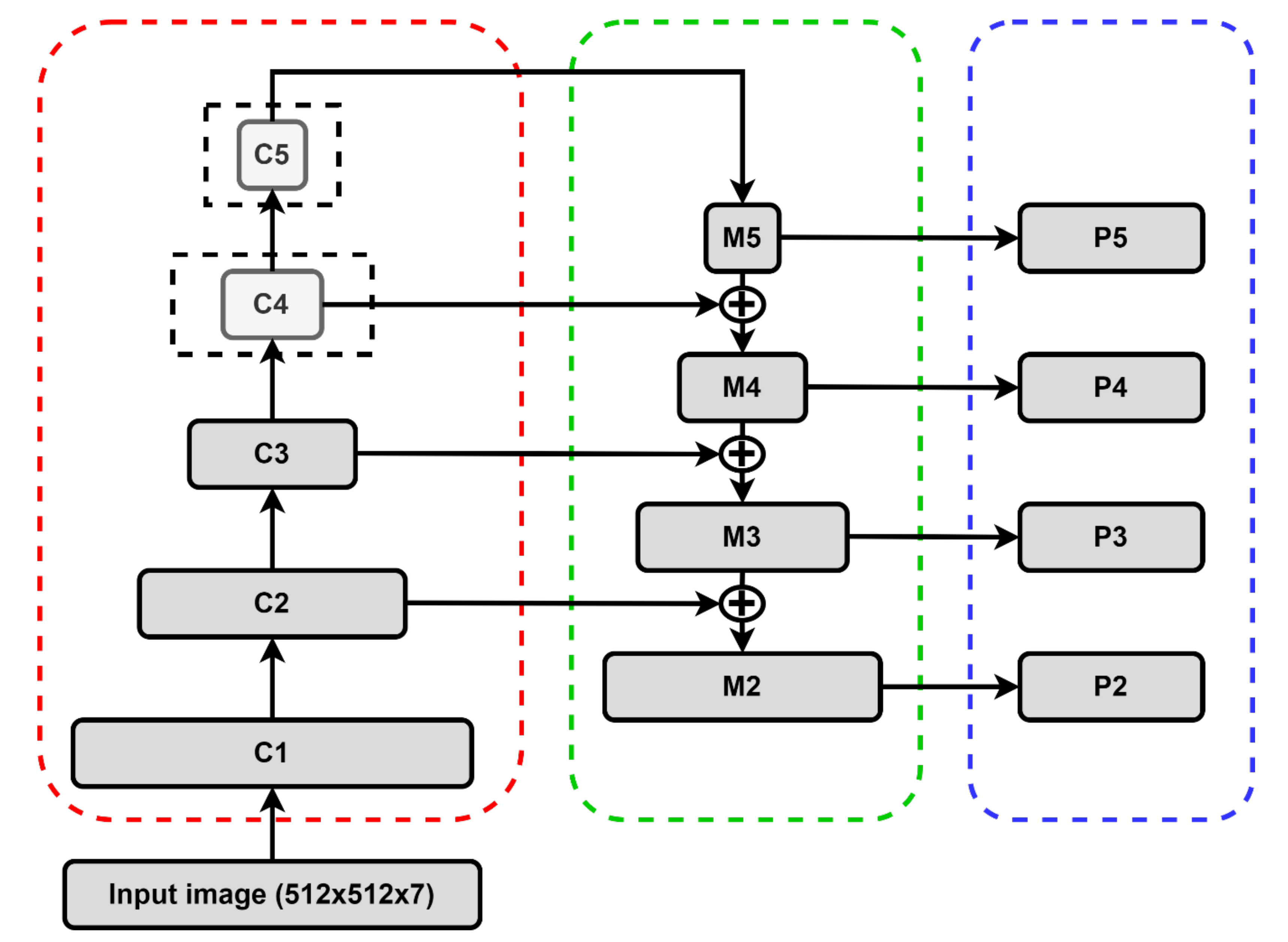
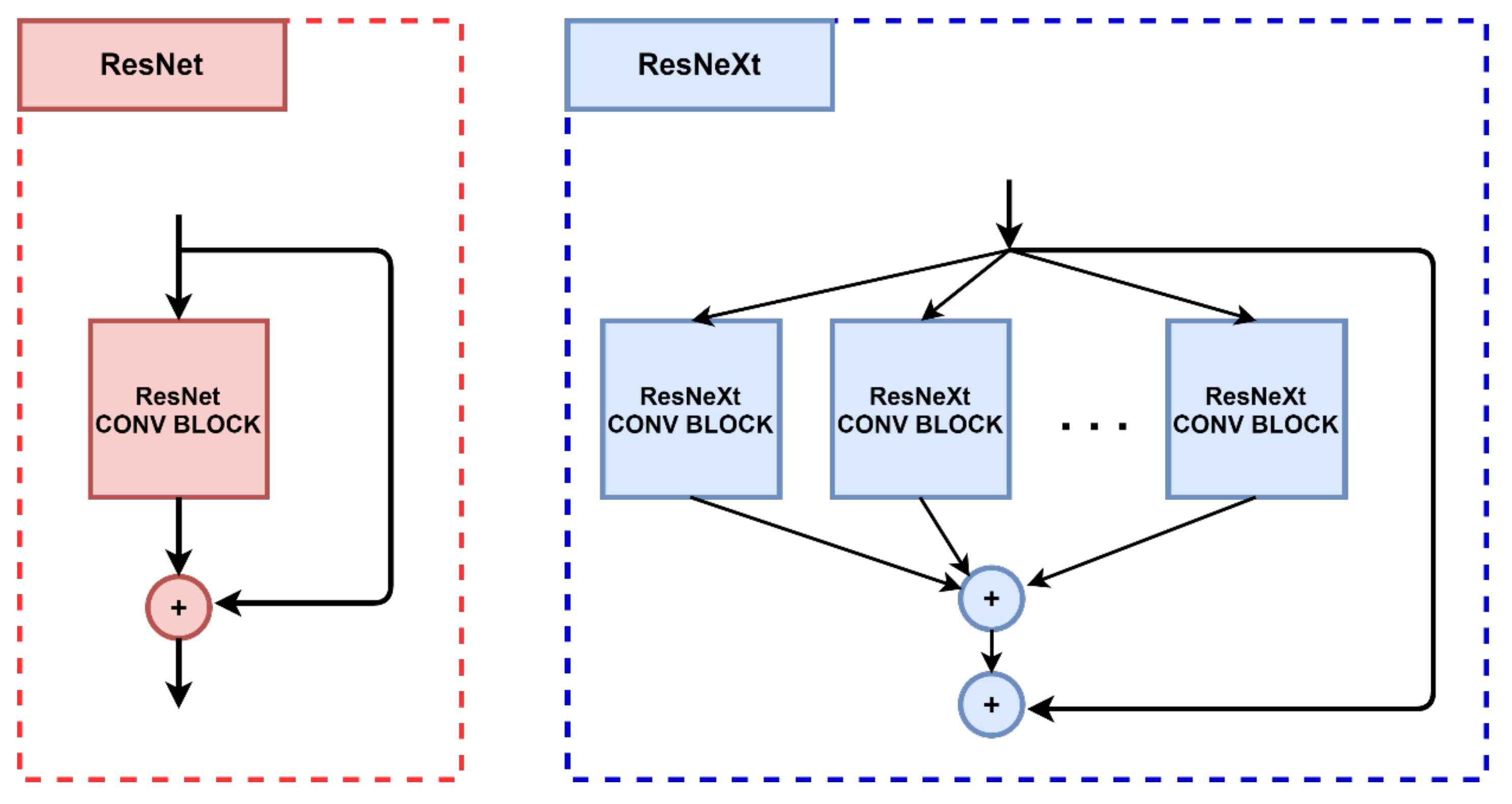
2.4.1. Backbone Structure
2.4.2. Region Proposal Network and Region of Interest (ROI) Align
2.4.3. Loss Functions
2.4.4. Hyperparameter Configuration
2.5. Accuracy Analysis
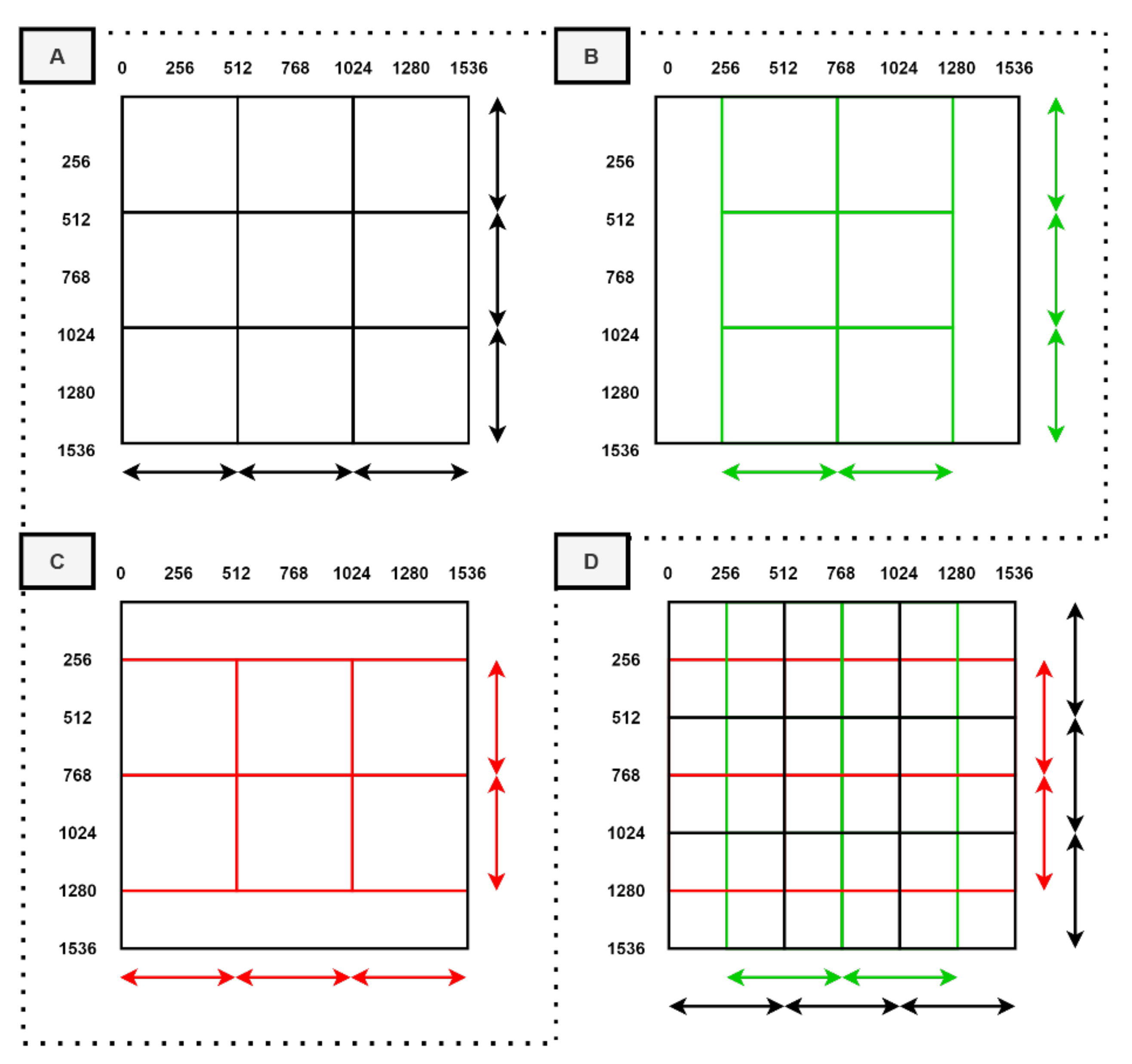
2.6. Scene Mosaicking
3. Results
3.1. Ground Truth COCO Transformation
3.2. Evaluation of COCO Metrics
3.3. Image Mosaicking
4. Discussion
5. Conclusions
Author Contributions
Funding
Acknowledgments
Conflicts of Interest
References
- Zhu, X.X.; Tuia, D.; Mou, L.; Xia, G.; Zhang, L.; Xu, F.; Fraundorfer, F. Deep Learning in Remote Sensing: A Comprehensive Review and List of Resources. IEEE Geosci. Remote Sens. Mag. 2017, 5, 8–36. [Google Scholar] [CrossRef]
- Liu, L.; Ouyang, W.; Wang, X.; Fieguth, P.; Chen, J.; Liu, X.; Pietikäinen, M. Deep Learning for Generic Object Detection: A Survey. Int. J. Comput. Vis. 2020, 128, 261–318. [Google Scholar] [CrossRef]
- Zhang, L.; Zhang, L.; Du, B. Deep learning for remote sensing data: A technical tutorial on the state of the art. IEEE Geosci. Remote Sens. Mag. 2016, 4, 22–40. [Google Scholar] [CrossRef]
- Nogueira, K.; Penatti, O.A.B.; dos Santos, J.A. Towards better exploiting convolutional neural networks for remote sensing scene classification. Pattern Recognit. 2017, 61, 539–556. [Google Scholar] [CrossRef]
- Ma, L.; Liu, Y.; Zhang, X.; Ye, Y.; Yin, G.; Johnson, B.A. Deep learning in remote sensing applications: A meta-analysis and review. ISPRS J. Photogramm. Remote Sens. 2019, 152, 166–177. [Google Scholar] [CrossRef]
- Zhang, L.; Li, W.; Shen, L.; Lei, D. Multilevel dense neural network for pan-sharpening. Int. J. Remote Sens. 2020, 41, 7201–7216. [Google Scholar] [CrossRef]
- Ma, J.; Yu, W.; Chen, C.; Liang, P.; Guo, X.; Jiang, J. Pan-GAN: An unsupervised pan-sharpening method for remote sensing image fusion. Inf. Fusion 2020, 62, 110–120. [Google Scholar] [CrossRef]
- Liu, L.; Wang, J.; Zhang, E.; Li, B.; Zhu, X.; Zhang, Y.; Peng, J. Shallow-Deep Convolutional Network and Spectral-Discrimination-Based Detail Injection for Multispectral Imagery Pan-Sharpening. IEEE J. Sel. Top. Appl. Earth Obs. Remote Sens. 2020, 13, 1772–1783. [Google Scholar] [CrossRef]
- Liu, X.; Liu, Q.; Wang, Y. Remote sensing image fusion based on two-stream fusion network. Inf. Fusion 2020, 55, 1–15. [Google Scholar] [CrossRef]
- Hughes, L.H.; Schmitt, M.; Zhu, X.X. Mining hard negative samples for SAR-optical image matching using generative adversarial networks. Remote Sens. 2018, 10, 1552. [Google Scholar] [CrossRef]
- Merkle, N.; Luo, W.; Auer, S.; Müller, R.; Urtasun, R. Exploiting deep matching and SAR data for the geo-localization accuracy improvement of optical satellite images. Remote Sens. 2017, 9, 586. [Google Scholar] [CrossRef]
- Wang, S.; Quan, D.; Liang, X.; Ning, M.; Guo, Y.; Jiao, L. A deep learning framework for remote sensing image registration. ISPRS J. Photogramm. Remote Sens. 2018, 145, 148–164. [Google Scholar] [CrossRef]
- Ye, F.; Xiao, H.; Zhao, X.; Dong, M.; Luo, W.; Min, W. Remote Sensing Image Retrieval Using Convolutional Neural Network Features and Weighted Distance. IEEE Geosci. Remote Sens. Lett. 2018, 15, 1535–1539. [Google Scholar] [CrossRef]
- De Bem, P.P.; de Carvalho Júnior, O.A.; de Carvalho, O.L.F.; Gomes, R.A.T.; Fontes Guimarães, R. Performance Analysis of Deep Convolutional Autoencoders with Different Patch Sizes for Change Detection from Burnt Areas. Remote Sens. 2020, 12, 2576. [Google Scholar] [CrossRef]
- De Bem, P.P.; de Carvalho Junior, O.; Fontes Guimarães, R.; Trancoso Gomes, R. Change Detection of Deforestation in the Brazilian Amazon Using Landsat Data and Convolutional Neural Networks. Remote Sens. 2020, 12, 901. [Google Scholar] [CrossRef]
- Zhang, P.; Gong, M.; Su, L.; Liu, J.; Li, Z. Change detection based on deep feature representation and mapping transformation for multi-spatial-resolution remote sensing images. ISPRS J. Photogramm. Remote Sens. 2016, 116, 24–41. [Google Scholar] [CrossRef]
- Peng, D.; Zhang, Y.; Guan, H. End-to-End Change Detection for High Resolution Satellite Images Using Improved UNet++. Remote Sens. 2019, 11, 1382. [Google Scholar] [CrossRef]
- Ammour, N.; Alhichri, H.; Bazi, Y.; Benjdira, B.; Alajlan, N.; Zuair, M. Deep Learning Approach for Car Detection in UAV Imagery. Remote Sens. 2017, 9, 312. [Google Scholar] [CrossRef]
- Chen, Y.; Li, Y.; Wang, J.; Chen, W.; Zhang, X. Remote Sensing Image Ship Detection under Complex Sea Conditions Based on Deep Semantic Segmentation. Remote Sens. 2020, 12, 625. [Google Scholar] [CrossRef]
- Dong, Z.; Lin, B. Learning a robust CNN-based rotation insensitive model for ship detection in VHR remote sensing images. Int. J. Remote Sens. 2020, 41, 3614–3626. [Google Scholar] [CrossRef]
- Yu, Y.; Gu, T.; Guan, H.; Li, D.; Jin, S. Vehicle Detection from High-Resolution Remote Sensing Imagery Using Convolutional Capsule Networks. IEEE Geosci. Remote Sens. Lett. 2019, 16, 1894–1898. [Google Scholar] [CrossRef]
- Diakogiannis, F.I.; Waldner, F.; Caccetta, P.; Wu, C. ResUNet-a: A deep learning framework for semantic segmentation of remotely sensed data. ISPRS J. Photogramm. Remote Sens. 2020, 162, 94–114. [Google Scholar] [CrossRef]
- Volpi, M.; Tuia, D. Deep multi-task learning for a geographically-regularized semantic segmentation of aerial images. ISPRS J. Photogramm. Remote Sens. 2018, 144, 48–60. [Google Scholar] [CrossRef]
- Zhao, W.; Du, S.; Wang, Q.; Emery, W.J. Contextually guided very-high-resolution imagery classification with semantic segments. ISPRS J. Photogramm. Remote Sens. 2017, 132, 48–60. [Google Scholar] [CrossRef]
- Wang, S.; Chen, W.; Xie, S.M.; Azzari, G.; Lobell, D.B. Weakly supervised deep learning for segmentation of remote sensing imagery. Remote Sens. 2020, 12, 207. [Google Scholar] [CrossRef]
- De Castro Filho, H.C.; de Carvalho Júnior, O.A.; de Carvalho, O.L.F.; de Bem, P.P.; dos Santos de Moura, R.; Olino de Albuquerque, A.; Rosa Silva, C.; Guimarães Ferreira, P.H.; Guimarães, R.F.; Gomes, R.A.T. Rice Crop Detection Using LSTM, Bi-LSTM, and Machine Learning Models from Sentinel-1 Time Series. Remote Sens. 2020, 12, 2655. [Google Scholar] [CrossRef]
- Ienco, D.; Interdonato, R.; Gaetano, R.; Ho Tong Minh, D. Combining Sentinel-1 and Sentinel-2 Satellite Image Time Series for land cover mapping via a multi-source deep learning architecture. ISPRS J. Photogramm. Remote Sens. 2019, 158, 11–22. [Google Scholar] [CrossRef]
- Interdonato, R.; Ienco, D.; Gaetano, R.; Ose, K. DuPLO: A DUal view Point deep Learning architecture for time series classification. ISPRS J. Photogramm. Remote Sens. 2019, 149, 91–104. [Google Scholar] [CrossRef]
- Zhong, L.; Hu, L.; Zhou, H. Deep learning based multi-temporal crop classification. Remote Sens. Environ. 2019, 221, 430–443. [Google Scholar] [CrossRef]
- Wieland, M.; Li, Y.; Martinis, S. Multi-sensor cloud and cloud shadow segmentation with a convolutional neural network. Remote Sens. Environ. 2019, 230, 111203. [Google Scholar] [CrossRef]
- Li, Z.; Shen, H.; Cheng, Q.; Liu, Y.; You, S.; He, Z. Deep learning based cloud detection for medium and high resolution remote sensing images of different sensors. ISPRS J. Photogramm. Remote Sens. 2019, 150, 197–212. [Google Scholar] [CrossRef]
- Xie, F.; Shi, M.; Shi, Z.; Yin, J.; Zhao, D. Multilevel cloud detection in remote sensing images based on deep learning. IEEE J. Sel. Top. Appl. Earth Obs. Remote Sens. 2017, 10, 3631–3640. [Google Scholar] [CrossRef]
- Li, Y.; Chen, W.; Zhang, Y.; Tao, C.; Xiao, R.; Tan, Y. Accurate cloud detection in high-resolution remote sensing imagery by weakly supervised deep learning. Remote Sens. Environ. 2020, 250, 112045. [Google Scholar] [CrossRef]
- Li, T.; Shen, H.; Yuan, Q.; Zhang, L. Geographically and temporally weighted neural networks for satellite-based mapping of ground-level PM2.5. ISPRS J. Photogramm. Remote Sens. 2020, 167, 178–188. [Google Scholar] [CrossRef]
- Park, Y.; Kwon, B.; Heo, J.; Hu, X.; Liu, Y.; Moon, T. Estimating PM2.5 concentration of the conterminous United States via interpretable convolutional neural networks. Environ. Pollut. 2020, 256, 113395. [Google Scholar] [CrossRef]
- Shen, H.; Li, T.; Yuan, Q.; Zhang, L. Estimating Regional Ground-Level PM 2.5 Directly From Satellite Top-Of-Atmosphere Reflectance Using Deep Belief Networks. J. Geophys. Res. Atmos. 2018, 123, 13875–13886. [Google Scholar] [CrossRef]
- Wen, C.; Liu, S.; Yao, X.; Peng, L.; Li, X.; Hu, Y.; Chi, T. A novel spatiotemporal convolutional long short-term neural network for air pollution prediction. Sci. Total Environ. 2019, 654, 1091–1099. [Google Scholar] [CrossRef]
- Carranza-García, M.; García-Gutiérrez, J.; Riquelme, J.C. A framework for evaluating land use and land cover classification using convolutional neural networks. Remote Sens. 2019, 11, 274. [Google Scholar] [CrossRef]
- Helber, P.; Bischke, B.; Dengel, A.; Borth, D. Eurosat: A novel dataset and deep learning benchmark for land use and land cover classification. IEEE J. Sel. Top. Appl. Earth Obs. Remote Sens. 2019, 12, 2217–2226. [Google Scholar] [CrossRef]
- Zhang, C.; Sargent, I.; Pan, X.; Li, H.; Gardiner, A.; Hare, J.; Atkinson, P.M. Joint Deep Learning for land cover and land use classification. Remote Sens. Environ. 2019, 221, 173–187. [Google Scholar] [CrossRef]
- Zhang, C.; Harrison, P.A.; Pan, X.; Li, H.; Sargent, I.; Atkinson, P.M. Scale Sequence Joint Deep Learning (SS-JDL) for land use and land cover classification. Remote Sens. Environ. 2020, 237, 111593. [Google Scholar] [CrossRef]
- Huang, B.; Zhao, B.; Song, Y. Urban land-use mapping using a deep convolutional neural network with high spatial resolution multispectral remote sensing imagery. Remote Sens. Environ. 2018, 214, 73–86. [Google Scholar] [CrossRef]
- Huang, F.; Yu, Y.; Feng, T. Automatic extraction of urban impervious surfaces based on deep learning and multi-source remote sensing data. J. Vis. Commun. Image Represent. 2019, 60, 16–27. [Google Scholar] [CrossRef]
- Li, W.; Liu, H.; Wang, Y.; Li, Z.; Jia, Y.; Gui, G. Deep Learning-Based Classification Methods for Remote Sensing Images in Urban Built-Up Areas. IEEE Access 2019, 7, 36274–36284. [Google Scholar] [CrossRef]
- Srivastava, S.; Vargas-Muñoz, J.E.; Tuia, D. Understanding urban landuse from the above and ground perspectives: A deep learning, multimodal solution. Remote Sens. Environ. 2019, 228, 129–143. [Google Scholar] [CrossRef]
- Li, X.; Liu, B.; Zheng, G.; Ren, Y.; Zhang, S.; Liu, Y.; Gao, L.; Liu, Y.; Zhang, B.; Wang, F. Deep learning-based information mining from ocean remote sensing imagery. Natl. Sci. Rev. 2020, nwaa047. [Google Scholar] [CrossRef]
- Arellano-Verdejo, J.; Lazcano-Hernandez, H.E.; Cabanillas-Terán, N. ERISNet: Deep neural network for Sargassum detection along the coastline of the Mexican Caribbean. PeerJ 2019, 7, e6842. [Google Scholar] [CrossRef]
- Guo, H.; Wei, G.; An, J. Dark Spot Detection in SAR Images of Oil Spill Using Segnet. Appl. Sci. 2018, 8, 2670. [Google Scholar] [CrossRef]
- Gao, Y.; Gao, F.; Dong, J.; Wang, S. Transferred Deep Learning for Sea Ice Change Detection From Synthetic-Aperture Radar Images. IEEE Geosci. Remote Sens. Lett. 2019, 16, 1655–1659. [Google Scholar] [CrossRef]
- Garcia-Garcia, A.; Orts-Escolano, S.; Oprea, S.; Villena-Martinez, V.; Garcia-Rodriguez, J. A Review on Deep Learning Techniques Applied to Semantic Segmentation. arXiv 2017, arXiv:1704.06857. [Google Scholar]
- Guo, Y.; Liu, Y.; Georgiou, T.; Lew, M.S. A review of semantic segmentation using deep neural networks. Int. J. Multimed. Inf. Retr. 2018, 7, 87–93. [Google Scholar] [CrossRef]
- Garcia-Garcia, A.; Orts-Escolano, S.; Oprea, S.; Villena-Martinez, V.; Martinez-Gonzalez, P.; Garcia-Rodriguez, J. A survey on deep learning techniques for image and video semantic segmentation. Appl. Soft Comput. 2018, 70, 41–65. [Google Scholar] [CrossRef]
- Geng, Q.; Zhou, Z.; Cao, X. Survey of recent progress in semantic image segmentation with CNNs. Sci. China Inf. Sci. 2018, 61, 1–18. [Google Scholar] [CrossRef]
- Lateef, F.; Ruichek, Y. Survey on semantic segmentation using deep learning techniques. Neurocomputing 2019, 338, 321–348. [Google Scholar] [CrossRef]
- Yu, H.; Yang, Z.; Tan, L.; Wang, Y.; Sun, W.; Sun, M.; Tang, Y. Methods and datasets on semantic segmentation: A review. Neurocomputing 2018, 304, 82–103. [Google Scholar] [CrossRef]
- He, K.; Gkioxari, G.; Dollar, P.; Girshick, R. Mask R-CNN. IEEE Trans. Pattern Anal. Mach. Intell. 2020, 42, 386–397. [Google Scholar] [CrossRef]
- Dai, J.; He, K.; Sun, J. Instance-Aware Semantic Segmentation via Multi-task Network Cascades. In Proceedings of the 2016 IEEE Conference on Computer Vision and Pattern Recognition (CVPR), Las Vegas, NV, USA, 26 June–1 July 2016; pp. 3150–3158. [Google Scholar]
- Pinheiro, P.O.; Collobert, R.; Dollar, P. Learning to Segment Object Candidates. In Proceedings of the 28th International Conference on Neural Information Processing Systems (NIPS’15), Montreal, QC, Canada, 7–12 December 2015; pp. 1990–1998. [Google Scholar]
- Pinheiro, P.O.; Lin, T.Y.; Collobert, R.; Dollár, P. Learning to refine object segments. In Proceedings of the 14th European Conference on Computer Vision (ECCV 2016), Amsterdam, The Netherlands, 11–14 October 2016; Volume 9905, pp. 75–91. [Google Scholar] [CrossRef]
- Arnab, A.; Torr, P.H.S. Pixelwise Instance Segmentation with a Dynamically Instantiated Network. In Proceedings of the 2017 IEEE Conference on Computer Vision and Pattern Recognition (CVPR), Honolulu, HI, USA, 21–26 July 2017; pp. 879–888. [Google Scholar]
- Bai, M.; Urtasun, R. Deep Watershed Transform for Instance Segmentation. In Proceedings of the 2017 IEEE Conference on Computer Vision and Pattern Recognition (CVPR), Honolulu, HI, USA, 21–26 July 2017; pp. 2858–2866. [Google Scholar]
- Kirillov, A.; Levinkov, E.; Andres, B.; Savchynskyy, B.; Rother, C. InstanceCut: From Edges to Instances with MultiCut. In Proceedings of the 2017 IEEE Conference on Computer Vision and Pattern Recognition (CVPR), Honolulu, HI, USA, 21–26 July 2017; pp. 7322–7331. [Google Scholar]
- Liu, S.; Qi, L.; Qin, H.; Shi, J.; Jia, J. Path Aggregation Network for Instance Segmentation. In Proceedings of the 2018 IEEE/CVF Conference on Computer Vision and Pattern Recognition, Salt Lake City, UT, USA, 18–23 June 2018; pp. 8759–8768. [Google Scholar]
- Li, Y.; Qi, H.; Dai, J.; Ji, X.; Wei, Y. Fully Convolutional Instance-Aware Semantic Segmentation. In Proceedings of the 2017 IEEE Conference on Computer Vision and Pattern Recognition (CVPR), Honolulu, HI, USA, 21–26 July 2017; pp. 4438–4446. [Google Scholar]
- Cai, Z.; Vasconcelos, N. Cascade R-CNN: Delving Into High Quality Object Detection. In Proceedings of the 2018 IEEE/CVF Conference on Computer Vision and Pattern Recognition, Salt Lake City, UT, USA, 18–23 June 2018; pp. 6154–6162. [Google Scholar]
- Chen, K.; Ouyang, W.; Loy, C.C.; Lin, D.; Pang, J.; Wang, J.; Xiong, Y.; Li, X.; Sun, S.; Feng, W.; et al. Hybrid Task Cascade for Instance Segmentation. In Proceedings of the 2019 IEEE/CVF Conference on Computer Vision and Pattern Recognition (CVPR), Long Beach, CA, USA, 16–21 June 2019; pp. 4969–4978. [Google Scholar]
- Huang, Z.; Huang, L.; Gong, Y.; Huang, C.; Wang, X. Mask Scoring R-CNN. In Proceedings of the 2019 IEEE/CVF Conference on Computer Vision and Pattern Recognition (CVPR), Long Beach, CA, USA, 16–21 June 2019; pp. 6402–6411. [Google Scholar]
- Su, H.; Wei, S.; Liu, S.; Liang, J.; Wang, C.; Shi, J.; Zhang, X. HQ-ISNet: High-Quality Instance Segmentation for Remote Sensing Imagery. Remote Sens. 2020, 12, 989. [Google Scholar] [CrossRef]
- Asgari Taghanaki, S.; Abhishek, K.; Cohen, J.P.; Cohen-Adad, J.; Hamarneh, G. Deep semantic segmentation of natural and medical images: A review. Artif. Intell. Rev. 2020. [Google Scholar] [CrossRef]
- Deng, S.; Zhang, X.; Yan, W.; Chang, E.I.C.; Fan, Y.; Lai, M.; Xu, Y. Deep learning in digital pathology image analysis: A survey. Front. Med. 2020. [Google Scholar] [CrossRef]
- Jiang, Y.; Li, C. Convolutional Neural Networks for Image-Based High-Throughput Plant Phenotyping: A Review. Plant. Phenomics 2020, 2020, 4152816. [Google Scholar] [CrossRef]
- Ruiz-Santaquiteria, J.; Bueno, G.; Deniz, O.; Vallez, N.; Cristobal, G. Semantic versus instance segmentation in microscopic algae detection. Eng. Appl. Artif. Intell. 2020, 87, 103271. [Google Scholar] [CrossRef]
- Qiao, Y.; Truman, M.; Sukkarieh, S. Cattle segmentation and contour extraction based on Mask R-CNN for precision livestock farming. Comput. Electron. Agric. 2019, 165, 104958. [Google Scholar] [CrossRef]
- Xu, B.; Wang, W.; Falzon, G.; Kwan, P.; Guo, L.; Chen, G.; Tait, A.; Schneider, D. Automated cattle counting using Mask R-CNN in quadcopter vision system. Comput. Electron. Agric. 2020, 171, 105300. [Google Scholar] [CrossRef]
- Champ, J.; Mora-Fallas, A.; Goëau, H.; Mata-Montero, E.; Bonnet, P.; Joly, A. Instance segmentation for the fine detection of crop and weed plants by precision agricultural robots. Appl. Plant. Sci. 2020, 8, 1–10. [Google Scholar] [CrossRef] [PubMed]
- Zhang, Q.; Liu, Y.; Gong, C.; Chen, Y.; Yu, H. Applications of Deep Learning for Dense Scenes Analysis in Agriculture: A Review. Sensors 2020, 20, 1520. [Google Scholar] [CrossRef]
- Yekeen, S.T.; Balogun, A.; Wan Yusof, K.B. A novel deep learning instance segmentation model for automated marine oil spill detection. ISPRS J. Photogramm. Remote Sens. 2020, 167, 190–200. [Google Scholar] [CrossRef]
- Li, Q.; Mou, L.; Hua, Y.; Sun, Y.; Jin, P.; Shi, Y.; Zhu, X.X. Instance segmentation of buildings using keypoints. arXiv 2020, arXiv:2006.03858. [Google Scholar]
- Wen, Q.; Jiang, K.; Wang, W.; Liu, Q.; Guo, Q.; Li, L.; Wang, P. Automatic Building Extraction from Google Earth Images under Complex Backgrounds Based on Deep Instance Segmentation Network. Sensors 2019, 19, 333. [Google Scholar] [CrossRef]
- Mou, L.; Zhu, X.X. Vehicle Instance Segmentation from Aerial Image and Video Using a Multitask Learning Residual Fully Convolutional Network. IEEE Trans. Geosci. Remote Sens. 2018, 56, 6699–6711. [Google Scholar] [CrossRef]
- Feng, Y.; Diao, W.; Zhang, Y.; Li, H.; Chang, Z.; Yan, M.; Sun, X.; Gao, X. Ship Instance Segmentation from Remote Sensing Images Using Sequence Local Context Module. In Proceedings of the 2019 IEEE International Geoscience and Remote Sensing Symposium (IGARSS 2019), Yokohama, Japan, 28 July–2 August 2019; pp. 1025–1028. [Google Scholar]
- Yu, Y.; Zhang, K.; Yang, L.; Zhang, D. Fruit detection for strawberry harvesting robot in non-structural environment based on Mask-RCNN. Comput. Electron. Agric. 2019, 163, 104846. [Google Scholar] [CrossRef]
- Wei, X.S.; Xie, C.W.; Wu, J.; Shen, C. Mask-CNN: Localizing parts and selecting descriptors for fine-grained bird species categorization. Pattern Recognit. 2018, 76, 704–714. [Google Scholar] [CrossRef]
- Audebert, N.; Le Saux, B.; Lefèvre, S. Beyond RGB: Very high resolution urban remote sensing with multimodal deep networks. ISPRS J. Photogramm. Remote Sens. 2018, 140, 20–32. [Google Scholar] [CrossRef]
- De Albuquerque, A.O.; de Carvalho Júnior, O.A.; de Carvalho, O.L.F.; de Bem, P.P.; Ferreira, P.H.G.; dos Santos de Moura, R.; Silva, C.R.; Trancoso Gomes, R.A.; Fontes Guimarães, R. Deep Semantic Segmentation of Center Pivot Irrigation Systems from Remotely Sensed Data. Remote Sens. 2020, 12, 2159. [Google Scholar] [CrossRef]
- Martins, V.S.; Kaleita, A.L.; Gelder, B.K.; da Silveira, H.L.F.; Abe, C.A. Exploring multiscale object-based convolutional neural network (multi-OCNN) for remote sensing image classification at high spatial resolution. ISPRS J. Photogramm. Remote Sens. 2020, 168, 56–73. [Google Scholar] [CrossRef]
- Yi, Y.; Zhang, Z.; Zhang, W.; Zhang, C.; Li, W.; Zhao, T. Semantic Segmentation of Urban Buildings from VHR Remote Sensing Imagery Using a Deep Convolutional Neural Network. Remote Sens. 2019, 11, 1774. [Google Scholar] [CrossRef]
- Audebert, N.; Le Saux, B.; Lefèvre, S. Segment-before-Detect: Vehicle Detection and Classification through Semantic Segmentation of Aerial Images. Remote Sens. 2017, 9, 368. [Google Scholar] [CrossRef]
- Mahdianpari, M.; Salehi, B.; Rezaee, M.; Mohammadimanesh, F.; Zhang, Y. Very Deep Convolutional Neural Networks for Complex Land Cover Mapping Using Multispectral Remote Sensing Imagery. Remote Sens. 2018, 10, 1119. [Google Scholar] [CrossRef]
- Russell, B.C.; Torralba, A.; Murphy, K.P.; Freeman, W.T. LabelMe: A Database and Web-Based Tool for Image Annotation. Int. J. Comput. Vis. 2008, 77, 157–173. [Google Scholar] [CrossRef]
- Deng, J.; Dong, W.; Socher, R.; Li, L.-J.; Kai, L.; Fei-Fei, L. ImageNet: A large-scale hierarchical image database. In Proceedings of the 2009 IEEE Conference on Computer Vision and Pattern Recognition, Miami, FL, USA, 22–24 June 2009; pp. 248–255. [Google Scholar]
- Everingham, M.; Eslami, S.M.A.; Van Gool, L.; Williams, C.K.I.; Winn, J.; Zisserman, A. The Pascal Visual Object Classes Challenge: A Retrospective. Int. J. Comput. Vis. 2015, 111, 98–136. [Google Scholar] [CrossRef]
- Cordts, M.; Omran, M.; Ramos, S.; Rehfeld, T.; Enzweiler, M.; Benenson, R.; Franke, U.; Roth, S.; Schiele, B. The Cityscapes Dataset for Semantic Urban Scene Understanding. In Proceedings of the 2016 IEEE Conference on Computer Vision and Pattern Recognition (CVPR), Las Vegas, NV, USA, 26 June–1 July 2016; Volume 29, pp. 3213–3223. [Google Scholar]
- Kuznetsova, A.; Rom, H.; Alldrin, N.; Uijlings, J.; Krasin, I.; Pont-Tuset, J.; Kamali, S.; Popov, S.; Malloci, M.; Kolesnikov, A.; et al. The Open Images Dataset V4. Int. J. Comput. Vis. 2020, 128, 1956–1981. [Google Scholar] [CrossRef]
- Lin, T.-Y.; Maire, M.; Belongie, S.; Hays, J.; Perona, P.; Ramanan, D.; Dollár, P.; Zitnick, C.L. Microsoft COCO: Common Objects in Context. In Proceedings of the 13th European Conference on Computer Vision (ECCV 2014), Zurich, Switzerland, 6–12 September 2014; Volume 8693, pp. 740–755, ISBN 978-3-319-10601-4. [Google Scholar]
- Wu, Y.; Kirillov, A.; Massa, F.; Lo, W.-Y.; Girshick, R. Detectron2. 2019. Available online: lhttps://github.com/facebookresearch/detectron2 (accessed on 14 November 2020).
- Rundquist, D.C.; Hoffman, R.O.; Carlson, M.P.; Cook, A.E. Nebraska center-pivot inventory: An example of operational satellite remote sensing on a long-term basis. Photogramm. Eng. Remote Sensing 1989, 55, 587–590. [Google Scholar]
- Heller, R.C.; Johnson, K.A. Estimating irrigated land acreage from Landsat imagery. Photogramm. Eng. Remote Sensing 1979, 45, 1379–1386. [Google Scholar]
- Agência Nacional de Águas. Levantamento da Agricultura Irrigada por Pivôs Centrais no Brasil (1985–2017); ANA: Brasilia, Brazil, 2019. [Google Scholar]
- Agência Nacional de Águas. Levantamento da Agricultura Irrigada por Pivôs Centrais no Brasil—2014: Relatório Síntese; ANA: Brasilia, Brazil, 2016; ISBN 9788582100349. [Google Scholar]
- Ferreira, E.; De Toledo, J.H.; Dantas, A.A.A.; Pereira, R.M. Cadastral maps of irrigated areas by center pivots in the State of Minas Gerais, using CBERS-2B/CCD satellite imaging. Eng. Agric. 2011, 31, 771–780. [Google Scholar] [CrossRef]
- Martins, J.D.; Bohrz, I.S.; Fredrich, M.; Veronez, R.P.; Kunz, G.A.; Tura, E.F. Levantamento da área irrigada por pivô central no Estado do Rio Grande do Sul. Irrig. Botucatu 2016, 21, 300–311. [Google Scholar] [CrossRef]
- Zhang, C.; Yue, P.; Di, L.; Wu, Z. Automatic Identification of Center Pivot Irrigation Systems from Landsat Images Using Convolutional Neural Networks. Agriculture 2018, 8, 147. [Google Scholar] [CrossRef]
- Saraiva, M.; Protas, É.; Salgado, M.; Souza, C. Automatic Mapping of Center Pivot Irrigation Systems from Satellite Images Using Deep Learning. Remote Sens. 2020, 12, 558. [Google Scholar] [CrossRef]
- Shermeyer, J.; Hossler, T.; van Etten, A.; Hogan, D.; Lewis, R.; Kim, D. RarePlanes: Synthetic Data Takes Flight. arXiv 2020, arXiv:2006.02963. [Google Scholar]
- Xia, G.; Bai, X.; Ding, J.; Zhu, Z.; Belongie, S.; Luo, J.; Datcu, M.; Pelillo, M.; Zhang, L. DOTA: A Large-Scale Dataset for Object Detection in Aerial Images. In Proceedings of the 2018 IEEE/CVF Conference on Computer Vision and Pattern Recognition, Salt Lake City, UT, USA, 18–23 June 2018; pp. 3974–3983. [Google Scholar]
- Zamir, S.W.; Arora, A.; Gupta, A.; Khan, S.; Sun, G.; Khan, F.S.; Zhu, F.; Shao, L.; Xia, G.S.; Bai, X. iSAID: A large-scale dataset for instance segmentation in aerial images. arXiv 2019, arXiv:1905.12886. [Google Scholar]
- Van Etten, A.; Lindenbaum, D.; Bacastow, T. SpaceNet: A remote sensing dataset and challenge series. arXiv 2018, arXiv:1807.01232. [Google Scholar]
- Althoff, D.; Rodrigues, L.N. The expansion of center-pivot irrigation in the cerrado biome. Irriga 2019, 1, 56–61. [Google Scholar] [CrossRef]
- Brunckhorst, A.; de Souza Bias, E. Aplicação de sig na gestão de conflitos pelo uso da água na porção goiana da bacia hidrográfica do rio são Marcos, município de Cristalina—GO. Geociencias 2014, 33, 23–31. [Google Scholar]
- Silva, L.M.D.C.; Da Hora, M.D.A.G.M. Conflito pelo Uso da Água na Bacia Hidrográfica do Rio São Marcos: O Estudo de Caso da UHE Batalha. Engevista 2014, 17, 166. [Google Scholar] [CrossRef]
- De Oliveira, S.N.; de Carvalho Júnior, O.A.; Gomes, R.A.T.; Guimarães, R.F.; McManus, C.M. Landscape-fragmentation change due to recent agricultural expansion in the Brazilian Savanna, Western Bahia, Brazil. Reg. Environ. Chang. 2017, 17, 411–423. [Google Scholar] [CrossRef]
- De Oliveira, S.N.; de Carvalho Júnior, O.A.; Trancoso Gomes, R.A.; Fontes Guimarães, R.; McManus, C.M. Deforestation analysis in protected areas and scenario simulation for structural corridors in the agricultural frontier of Western Bahia, Brazil. Land Use Policy 2017, 61, 40–52. [Google Scholar] [CrossRef]
- Pousa, R.; Costa, M.H.; Pimenta, F.M.; Fontes, V.C.; Castro, M. Climate change and intense irrigation growth in Western Bahia, Brazil: The urgent need for hydroclimatic monitoring. Water 2019, 11, 933. [Google Scholar] [CrossRef]
- Kelly, A. Cocosynth. Available online: https://github.com/akTwelve/cocosynth (accessed on 30 August 2020).
- He, K.; Gkioxari, G.; Dollar, P.; Girshick, R. Mask R-CNN. In Proceedings of the 2017 IEEE International Conference on Computer Vision (ICCV), Venice, Italy, 22–29 October 2017; pp. 2980–2988. [Google Scholar]
- Girshick, R.; Donahue, J.; Darrell, T.; Malik, J. Rich Feature Hierarchies for Accurate Object Detection and Semantic Segmentation. In Proceedings of the 2014 IEEE Conference on Computer Vision and Pattern Recognition, Columbus, OH, USA, 23–28 June 2014; Volume 1, pp. 580–587. [Google Scholar]
- Girshick, R. Fast R-CNN. In Proceedings of the 2015 IEEE International Conference on Computer Vision (ICCV), Santiago, Chile, 7–13 December 2015; pp. 1440–1448. [Google Scholar]
- Ren, S.; He, K.; Girshick, R.; Sun, J. Faster R-CNN: Towards Real-Time Object Detection with Region Proposal Networks. IEEE Trans. Pattern Anal. Mach. Intell. 2017, 39, 1137–1149. [Google Scholar] [CrossRef]
- He, K.; Zhang, X.; Ren, S.; Sun, J. Deep Residual Learning for Image Recognition. In Proceedings of the 2016 IEEE Conference on Computer Vision and Pattern Recognition (CVPR), Las Vegas, NV, USA, 26 June–1 July 2016; Volume 45, pp. 770–778. [Google Scholar]
- Xie, S.; Girshick, R.; Dollar, P.; Tu, Z.; He, K. Aggregated Residual Transformations for Deep Neural Networks. In Proceedings of the 2017 IEEE Conference on Computer Vision and Pattern Recognition (CVPR), Honolulu, HI, USA, 21–26 July 2017; pp. 5987–5995. [Google Scholar]
- Lin, T.-Y.; Dollar, P.; Girshick, R.; He, K.; Hariharan, B.; Belongie, S. Feature Pyramid Networks for Object Detection. In Proceedings of the 2017 IEEE Conference on Computer Vision and Pattern Recognition (CVPR), Honolulu, HI, USA, 21–26 July 2017; pp. 936–944. [Google Scholar]
- Girshick, R.; Donahue, J.; Darrell, T.; Malik, J. Region-Based Convolutional Networks for Accurate Object Detection and Segmentation. IEEE Trans. Pattern Anal. Mach. Intell. 2016, 38, 142–158. [Google Scholar] [CrossRef]
- Dai, Z.; Heckel, R. Channel Normalization in Convolutional Neural Network avoids Vanishing Gradients. arXiv 2019, arXiv:1907.09539. [Google Scholar]
- Bolya, D.; Zhou, C.; Xiao, F.; Lee, Y.J. YOLACT: Real-Time Instance Segmentation. In Proceedings of the 2019 IEEE/CVF International Conference on Computer Vision (ICCV), Seoul, Korea, 27 October–2 November 2019; pp. 9156–9165. [Google Scholar]
- Bolya, D.; Zhou, C.; Xiao, F.; Lee, Y.J. YOLACT++: Better Real-time Instance Segmentation. IEEE Trans. Pattern Anal. Mach. Intell. 2020, 1. [Google Scholar] [CrossRef]
- Zhao, W.; Du, S.; Emery, W.J. Object-Based Convolutional Neural Network for High-Resolution Imagery Classification. IEEE J. Sel. Top. Appl. Earth Obs. Remote Sens. 2017, 10, 3386–3396. [Google Scholar] [CrossRef]
- Zhang, C.; Sargent, I.; Pan, X.; Li, H.; Gardiner, A.; Hare, J.; Atkinson, P.M. An object-based convolutional neural network (OCNN) for urban land use classification. Remote Sens. Environ. 2018, 216, 57–70. [Google Scholar] [CrossRef]
- Deng, Z.; Sun, H.; Zhou, S.; Zhao, J.; Lei, L.; Zou, H. Multi-scale object detection in remote sensing imagery with convolutional neural networks. ISPRS J. Photogramm. Remote Sens. 2018, 145, 3–22. [Google Scholar] [CrossRef]
- Su, H.; Wei, S.; Yan, M.; Wang, C.; Shi, J.; Zhang, X. Object Detection and Instance Segmentation in Remote Sensing Imagery Based on Precise Mask R-CNN. In Proceedings of the 2019 IEEE International Geoscience and Remote Sensing Symposium (IGARSS 2019), Yokohama, Japan, 28 July–2 August 2019; pp. 1454–1457. [Google Scholar]
- Pang, J.; Li, C.; Shi, J.; Xu, Z.; Feng, H. R2-CNN: Fast Tiny Object Detection in Large-Scale Remote Sensing Images. IEEE Trans. Geosci. Remote Sens. 2019, 57, 5512–5524. [Google Scholar] [CrossRef]
- Li, K.; Wan, G.; Cheng, G.; Meng, L.; Han, J. Object detection in optical remote sensing images: A survey and a new benchmark. ISPRS J. Photogramm. Remote Sens. 2020, 159, 296–307. [Google Scholar] [CrossRef]
- Zhao, K.; Kang, J.; Jung, J.; Sohn, G. Building Extraction from Satellite Images Using Mask R-CNN with Building Boundary Regularization. In Proceedings of the 2018 IEEE/CVF Conference on Computer Vision and Pattern Recognition, Salt Lake City, UT, USA, 18–23 June 2018; pp. 242–246. [Google Scholar]


| Number of Images | Number of Instances | |
|---|---|---|
| Train | 228 | 4762 |
| Validation | 50 | 650 |
| Test | 50 | 850 |
| Backbone | Type | AP | AP50 | AP75 | APsmall | APmedium | AR100 |
|---|---|---|---|---|---|---|---|
| Resnet50-FPN | Mask | 70.567 | 86.095 | 81.150 | 56.214 | 77.494 | 75.2 |
| Box | 69.142 | 86.425 | 82.452 | 57.154 | 78.110 | 74.7 | |
| Resnet50-DC5 | Mask | 65.28 | 81.722 | 79.185 | 43.874 | 75.344 | 72.3 |
| Box | 63.017 | 82.435 | 80.746 | 48.541 | 72.554 | 70.4 | |
| Resnet50-C4 | Mask | 67.835 | 82.334 | 82.294 | 50.233 | 78.400 | 73.1 |
| Box | 65.561 | 83.390 | 81.162 | 49.392 | 74.963 | 70.9 | |
| Resnet101-FPN | Mask | 75.213 | 90.915 | 87.601 | 64.564 | 83.047 | 80.6 |
| Box | 74.415 | 91.618 | 87.806 | 64.715 | 80.978 | 80.1 | |
| Renset101-DC5 | Mask | 74.408 | 90.542 | 86.151 | 62.163 | 82.615 | 78.8 |
| Box | 73.624 | 90.343 | 86.390 | 62.421 | 81.037 | 78.6 | |
| Resnet101-C4 | Mask | 74.776 | 90.765 | 86.611 | 62.665 | 83.370 | 79.0 |
| Box | 73.814 | 90.473 | 86.868 | 62.846 | 81.161 | 78.9 | |
| ResneXt101-FPN | Mask | 77.970 | 93.758 | 90.620 | 67.585 | 84.776 | 82.3 |
| Box | 77.433 | 93.651 | 90.459 | 68.545 | 82.933 | 82.1 |
| Backbone | Type | AP | AP50 | AP75 | APsmall | APmedium | AR100 |
|---|---|---|---|---|---|---|---|
| ResneXt101-FPN | Mask | 74.776 | 92.417 | 87.605 | 64.619 | 81.781 | 78.8 |
| Box | 74.562 | 92.928 | 88.506 | 65.947 | 80.394 | 78.4 |
Publisher’s Note: MDPI stays neutral with regard to jurisdictional claims in published maps and institutional affiliations. |
© 2020 by the authors. Licensee MDPI, Basel, Switzerland. This article is an open access article distributed under the terms and conditions of the Creative Commons Attribution (CC BY) license (http://creativecommons.org/licenses/by/4.0/).
Share and Cite
Carvalho, O.L.F.d.; de Carvalho Júnior, O.A.; Albuquerque, A.O.d.; Bem, P.P.d.; Silva, C.R.; Ferreira, P.H.G.; Moura, R.d.S.d.; Gomes, R.A.T.; Guimarães, R.F.; Borges, D.L. Instance Segmentation for Large, Multi-Channel Remote Sensing Imagery Using Mask-RCNN and a Mosaicking Approach. Remote Sens. 2021, 13, 39. https://doi.org/10.3390/rs13010039
Carvalho OLFd, de Carvalho Júnior OA, Albuquerque AOd, Bem PPd, Silva CR, Ferreira PHG, Moura RdSd, Gomes RAT, Guimarães RF, Borges DL. Instance Segmentation for Large, Multi-Channel Remote Sensing Imagery Using Mask-RCNN and a Mosaicking Approach. Remote Sensing. 2021; 13(1):39. https://doi.org/10.3390/rs13010039
Chicago/Turabian StyleCarvalho, Osmar Luiz Ferreira de, Osmar Abílio de Carvalho Júnior, Anesmar Olino de Albuquerque, Pablo Pozzobon de Bem, Cristiano Rosa Silva, Pedro Henrique Guimarães Ferreira, Rebeca dos Santos de Moura, Roberto Arnaldo Trancoso Gomes, Renato Fontes Guimarães, and Díbio Leandro Borges. 2021. "Instance Segmentation for Large, Multi-Channel Remote Sensing Imagery Using Mask-RCNN and a Mosaicking Approach" Remote Sensing 13, no. 1: 39. https://doi.org/10.3390/rs13010039
APA StyleCarvalho, O. L. F. d., de Carvalho Júnior, O. A., Albuquerque, A. O. d., Bem, P. P. d., Silva, C. R., Ferreira, P. H. G., Moura, R. d. S. d., Gomes, R. A. T., Guimarães, R. F., & Borges, D. L. (2021). Instance Segmentation for Large, Multi-Channel Remote Sensing Imagery Using Mask-RCNN and a Mosaicking Approach. Remote Sensing, 13(1), 39. https://doi.org/10.3390/rs13010039