1. Introduction
Grapevines are highly sensitive to environmental conditions, which influence yield, grape composition, wine quality and wine style [
1]. The concept of “terroir” represents the combined effects of soil, climate, topography and human factors (e.g., viticultural management, choice of cultivar). Among the many climatic variables that influence grapevine physiology and phenology, temperature is often considered the most important [
2,
3,
4].
Bioclimatic indices calculated from climate data are the most common way to identify impacts of climate on grapevine growth. They are used to classify and compare winegrowing regions based on cumulative air temperature (e.g., Winkler index (WI), Huglin index (HI), Jones index) [
5,
6,
7] and can also be combined with phenological stages [
8]. Temperatures may vary greatly at fine scales [
9,
10]. Atmospheric parameters at the boundary layer depend on surface conditions (e.g., roughness, type), which can cause high spatial variability over relatively small areas (i.e., a few square meters to a few square kilometers). Local factors (e.g., slope, exposure, type of soil, distance from the ocean) cause temperature variations that exceed climate variability at a larger scale. This spatial variability in temperature often provides optimal conditions for grapevine growth and gives a winegrowing terroir its specific characteristics [
11]. Thus, improved knowledge of local climate variability is essential to better recommend and implement adaptation strategies in response to climate change.
Previous studies have highlighted the potential and usefulness of fine-scale climate modelling in vineyards [
12,
13,
14,
15,
16] that considers the main elements of the local environment. A statistical climate modelling method at local scale has been developed in these previous studies to model daily air temperatures (point) based on local factors as predictors, i.e., elevation, slope, geographical coordinates and exposition [
13]. At the seasonal scale, bioclimatic indices are generally mapped using spatial interpolation or spatialization of air temperature collected from a network [
17]. However, using temperature sensor networks limits research on vineyards, requiring several years of data and network management, raising the issue of mapping larger areas. Thermal remote sensing data with high temporal resolution is an interesting alternative. Several studies have demonstrated the utility of methods for “downscaling” land surface temperature (LST) derived at low spatial resolutions from remote sensing to improve the precision of these data by using robust statistical methods and predictors (e.g., topography, vegetation characteristics) [
18,
19,
20,
21]. The availability of spatially and temporally continuous temperature time series at high spatial and temporal resolution is crucial for a wide range of applications.
LST is a key parameter in the physics of land surface processes from local to global scales. However, using LST from thermal infrared data acquired remotely remains a challenge. A relationship between LST and air temperature exists and is well studied, but it depends on the thermal product used, the types of applications and the validation data [
22,
23,
24,
25,
26]. A previous study of applying LST to viticulture highlighted LST’s potential by analyzing the correlation between air temperature and LST for one growing season (2017–2018) without spatial or temporal reconstruction in the Waipara Valley (New Zealand) [
27].
To use LST [
28], daily time series often need to be reconstructed due to a lack of data (i.e., due to clouds, atmospheric conditions or other low-quality data). Reconstructing a time series in remote sensing depends on the revisit time and availability of data. Previous studies have examined two approaches for using spatially and temporally continuous LST time series: statistical methods and physical methods [
18,
20,
29,
30,
31,
32,
33].
The main objective of this study was to define the optimal spatial resolution for mapping bioclimatic indices when downscaling MODIS thermal satellite imagery. The study had three goals: (1) reconstruct daily time series of LST from 2012–2018, (2) downscale LST using topographic variables (slope, elevation, exposure, coordinates) using a support vector machine (SVM) algorithm and (3) evaluate the accuracy of using bioclimatic indices calculated from spatialized air temperature or downscaled LST (daily and weekly separately) using the identical method model [
13] of the previous studies.
2. Materials and Methods
2.1. Study Site and Data Collection
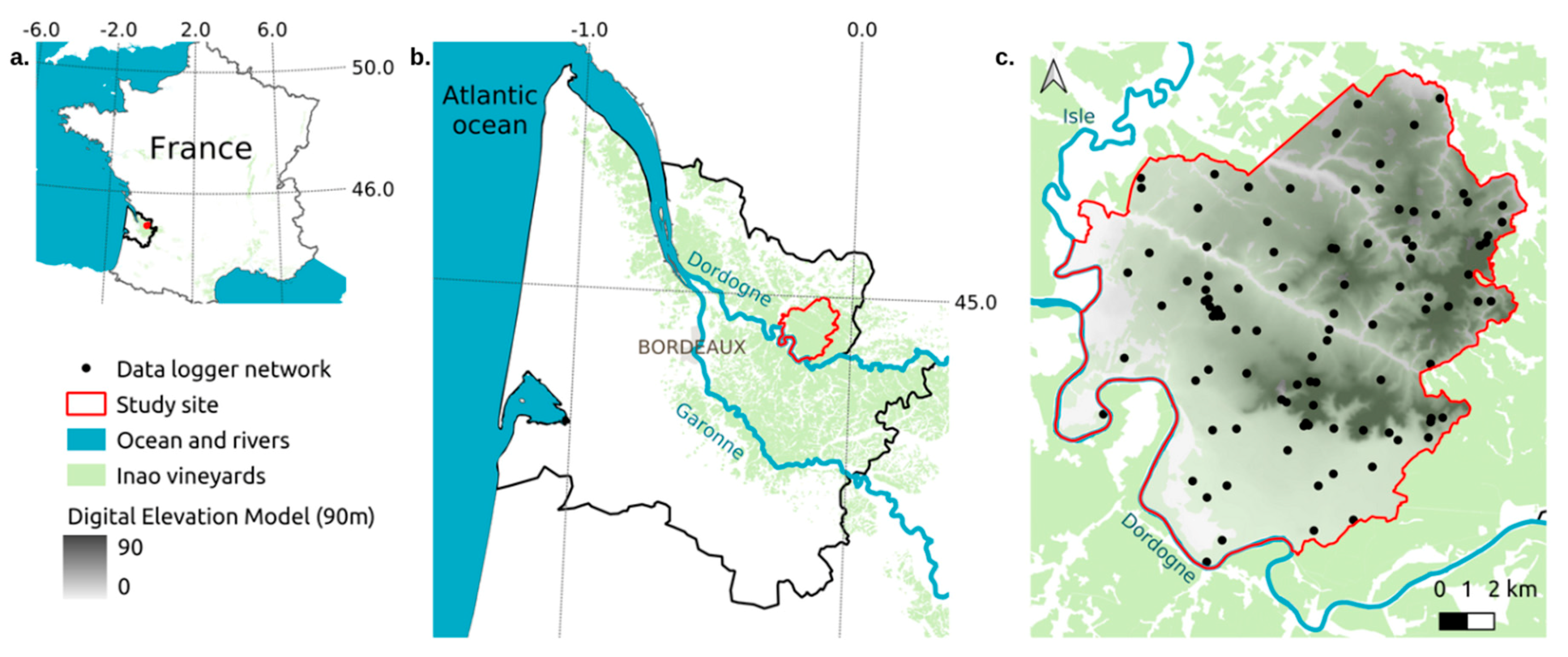
The study site was the vineyards of Saint-Emilion and Pomerol, in the winegrowing region of Bordeaux, in southwestern France (
Figure 1). It is bounded to the north by the Gironde administrative department and to the south by the Dordogne River. Its oceanic temperate climate, classified as Cfb (i.e., mild temperate, fully humid, warm summer) in the Köppen classification [
34], combined with a topographic context that ranges from 10–100 m with different soil types, provides suitable conditions for growing grapevines. This winegrowing region has been documented in detail in many studies of impacts of climate change on vineyards to climate change and their adaptation to it [
13,
35,
36,
37,
38]. The present study focused on the winegrowing period (i.e., March to October) of 2002–2018.
Elevation data (
Table 1) came from the Shuttle Radar Topography Mission (SRTM—NASA) at two resolutions: 1 arc-second for global coverage (~30 m) and 3 arc-seconds for global coverage (~90 m) [
39] and from Global Multi-resolution Terrain Elevation Data (GMTED2010) [
40] at the resolutions of 7.5 arc-seconds (~250 m), 15 arc-seconds (~500 m) and 30 arc-seconds (~1000 m). The data were downloaded from EarthExplorer (
https://earthexplorer.usgs.gov/). Topographic variables were derived from the digital elevation models (DEMs): elevation (m), slope (°), north-south orientation (°), east-west orientation (°) and geographic coordinates (latitude/longitude).
Air temperature data (
Table 1) came from a network of 90 air temperature data loggers, installed in the grapevine canopy 1.5 m from the ground, that recorded minimum and maximum air temperatures at hourly intervals. The network was installed in 2012 to consider the variety of local topographic parameters to better represent their influence on the local climate; it was also used for validation in previous studies [
13,
41].
LST data (
Table 1) was acquired using thermal remote sensing by the Terra (MOD) and Aqua (MYD) satellites with the MODIS sensor on board. Two satellites provide four daily LST datasets (two daytime and two nighttime). Two types of products were used: MOD11A1/MY11A1 (i.e., M*D11A1) (daily) and MOD11A2/MYD11A2 (i.e., M*D11A2) (8-day averaged composite). These data were downloaded via AppEars (
https://lpdaacsvc.cr.usgs.gov/appeears/) for the Gironde department from 2012–2018.
We used this dataset to calculate the common bioclimatic indices used in viticulture studies. Most are based on the sum of daily temperatures over a baseline temperature, which corresponded to the minimum vegetative temperature of 10 °C in this study [
5,
6,
8,
42].
2.2. Reconstruction and Downscaling of Daily LST Time Series
The weekly 1000 m LST averaged over 8 days (M*D11A2) [
43] were duplicated to create the daily LST for 8 days. The data missing from the daily LST at 1000 m (M*D11A1) [
44] were reconstructed with the available weekly LST data to create the daily LST time series. To decrease dependence on before and after temporal window reconstruction, this study replaced missing values with the 8-day composite values. The spatialization method (air temperature) and downscaling method (LST) were based on two assumptions: (1) temperature is related to topographic variables and can be modeled by machine-learning regression models and (2) a daily regression model that uses an SVM approach can predict (a) air temperature and (b) LST based on the topographic environment.
An SVM algorithm was used as a machine-learning regression model. We used the SVM initially developed by Cortes and Vapnik [
45] for classification studies, which uses a hyperplane to classify the input variables into an n-dimensional feature space with a maximum margin. We used the packages
caret [
46] and
e1071 [
47] of R software, version 4.0.1 (R Core Team, June 2020) to perform the regression using a radial kernel. Optimal values of the hyperparameters (cost and epsilon) were determined using 5-fold cross-validation, as developed in [
48] for spatializing air temperature.
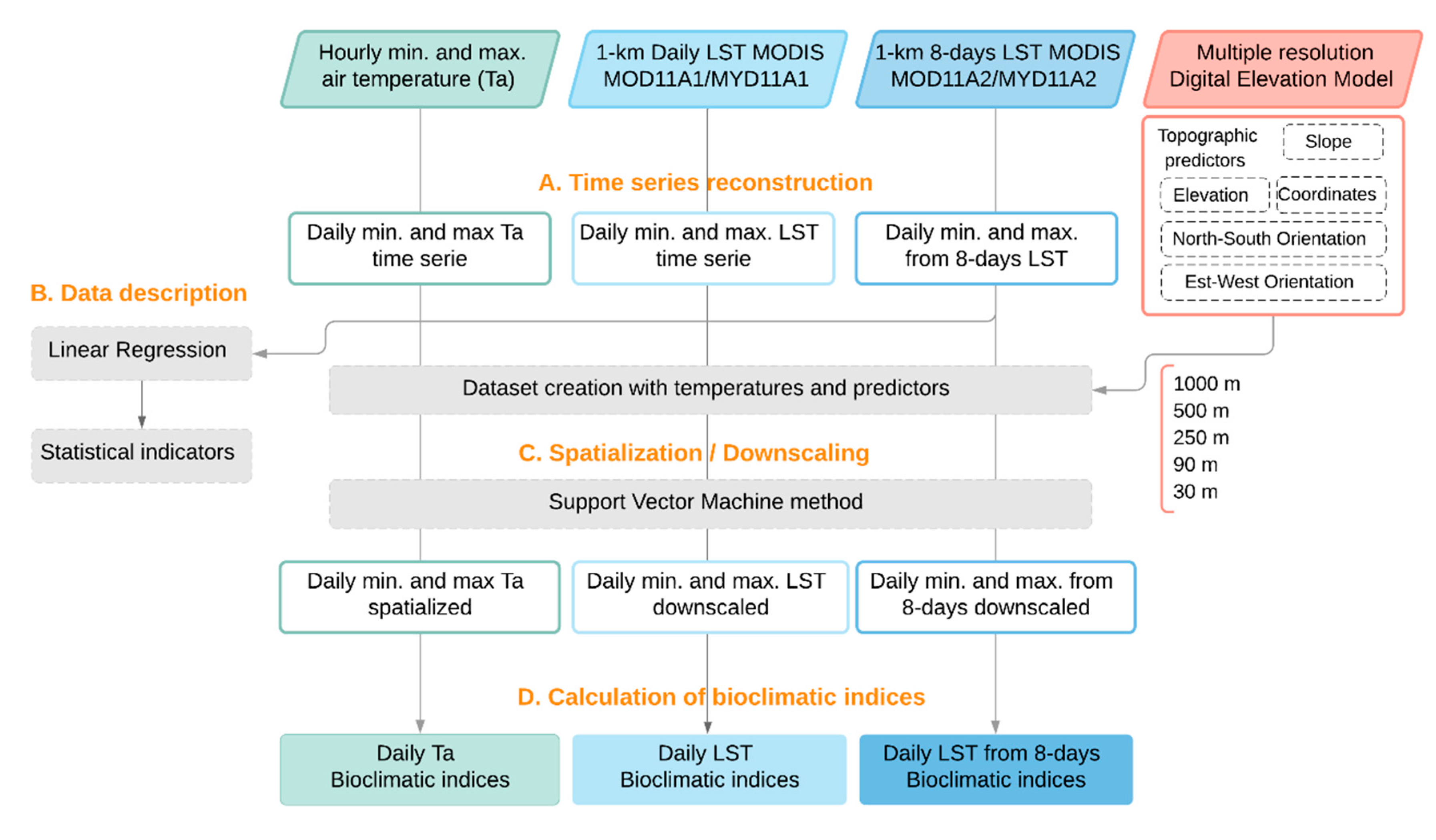
This study was based on four types of data: daily air temperatures, daily LST at 1000 m, weekly LST at 1000 m (i.e. chronology detailed in
Figure 2) and DEMs (1000, 500, 250, 90 and 30 m). The method had four steps (
Figure 3):
- A.
Create two daily time series for each type of data (hourly air temperature, daily LST and weekly LST): minima and maxima (
Figure 3A). These time series were created and calculated according to their time of acquisition (
Figure 2). If more than 60% of daily MODIS data were missing, they were reconstructed from the weekly MODIS data. The weekly MODIS data were duplicated to create the daily time series needed for the bioclimatic indices. In parallel, topographic variables were extracted from the DEMs at multiple resolutions (1000, 500, 250, 90 and 30 m): elevation, slope, north-south and east-west orientations and coordinates (latitude/longitude).
- B.
Analyze linear relationships between minimum and maximum air temperature and minimum, maximum (and their mean) (1) daily LST (M*D11A1) and (2) daily LST from the weekly data (M*D11A2) (
Figure 3B).
- C.
Spatialize air temperature and downscale LST with the SVM algorithm using topographic variables as predictors. Each modeled day of the growing season was trained with hyperparameters and determined by 5-fold cross-validation (
Figure 3C). The spatialized predictions at the daily scale were exported in raster format.
- D.
Calculate, from the predicted daily data, the seasonal WI and HI for the three types of data: air temperature, daily LST and daily LST from weekly data (
Figure 3D).
2.3. Bioclimatic Indices
The first index used was the standard index for growing degree-days (GDD), also known as
WI [
49]. It equals the sum of daily mean temperature greater than 10 °C during the seven months of the growing season (1 April to 31 October, Northern Hemisphere). This index enables several regions of the world to be compared [
5].
The heliothermal
HI [
6] is calculated using daily mean and maximum temperatures greater than 10 °C over six months of the growing season (1 April to 30 September, Northern Hemisphere) and includes a coefficient (k, 1.03 in this study) to adjust the day length as a function of the latitude.
2.4. Relationship between Daily Air Temperature and Daily LST from Daily and 8-Day Composite MODIS Products
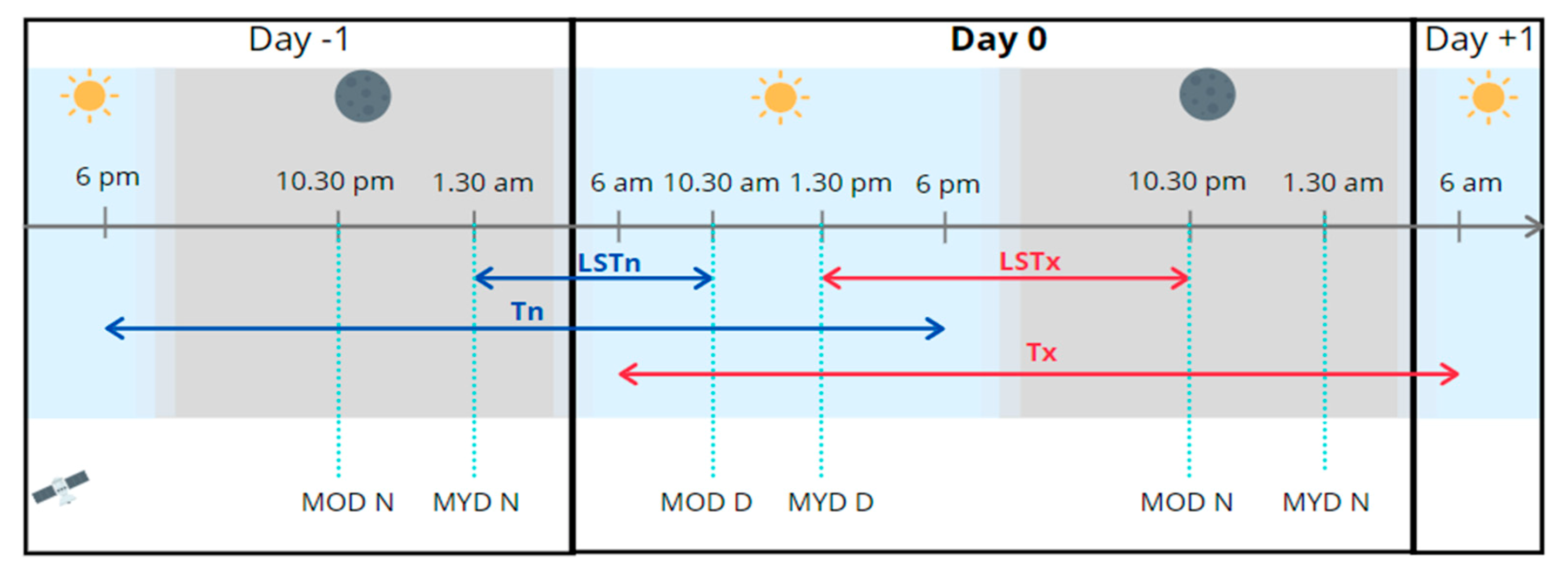
We studied the daily relationship between air temperature and LST per year for the 90 sensor locations that recorded air temperature and the two types of MODIS data extracted for these same locations: daily LST (M*D11A1) and 8-day composite LST (M*D11A2) transformed into daily time series. Thus, each of these two products contained two nighttime datasets and two daytime datasets.
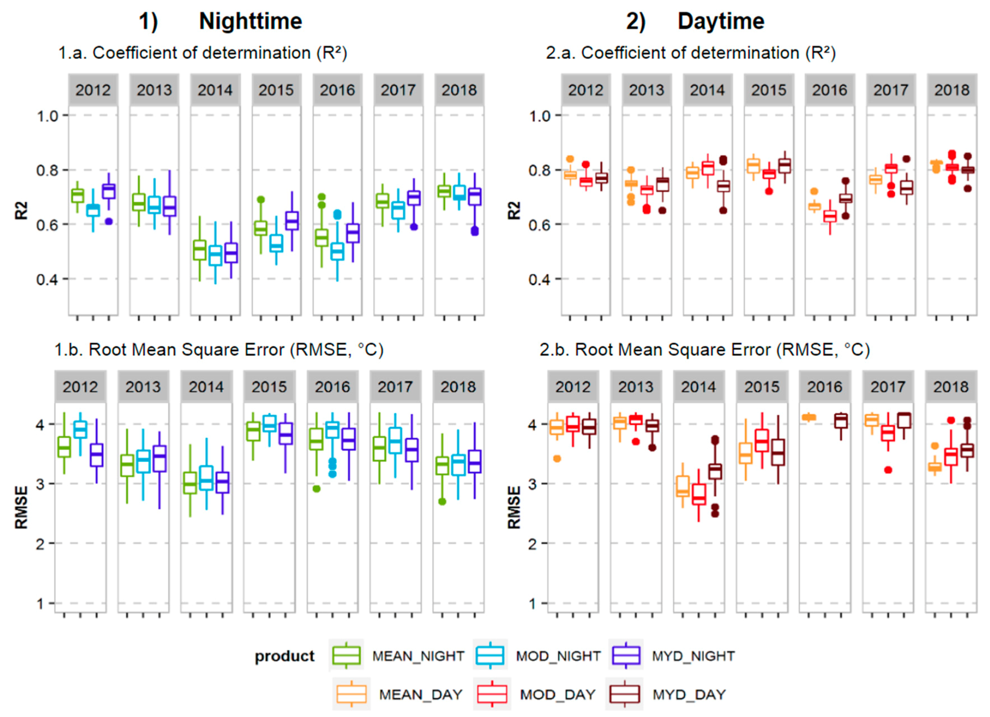
This first step analyzed the influence of the time of satellite passage on the LST, to obtain the best estimates of minimum and maximum air temperatures using statistical indicators such as coefficient of determination (i.e., R2) and root mean square error (i.e., RMSE). Each type of MODIS data and their mean (when both were available) were related to the daily minimum air temperature for nighttime data (MOD_NIGHT, MYD_NIGHT and MEAN_NIGHT, respectively) and to the daily maximum air temperature for daytime data (MOD_DAY, MYD_DAY and MEAN_DAY, respectively). Moreover, to verify the spatial distribution between bioclimatic indices values from temperature and LST by resolutions, Pearson correlation tests were computed after checking visually the normality of the distribution of indices.
3. Results
Coefficients of determination (R
2) of the linear relation between daily air temperature and LST (M*D11A1) were slightly higher for daytime (R
2 = 0.47–0.93) than for nighttime data (
Figure 4). Several studies have used linear regression to demonstrate the strong relationship between air temperatures and MODIS LST in different geographical contexts and time series lengths. For example, overpass timing influenced accuracy [
50], Aqua and Terra satellites had similar accuracy [
51,
52], one satellite was more accurate than the other [
53,
54] or nighttime data were more accurate than daytime data [
22,
55]. Both nighttime and daytime data showed that the mean of data from the two satellites (Aqua and Terra) stabilized the variability by maintaining a strong relationship while requiring less than half of the amount of data (mean of 90 observations vs. 160 observations for each MODIS product).
Linear relationships between daily LST from the 8-day composite (M*D11A2) and daily air temperatures showed, like for daily LST, slightly better results for daytime data than nighttime data, with higher R
2 and lower RMSE) (
Figure 5). Most results were not as good as those for the daily LST data. Since weekly data were pixel-averaged over 8 days, they were more repetitive than daily data and had less variable temperature. Peaks in minimum or maximum temperatures during each day were less visible (
Figure 4 Results varied greatly among years. For example, the mean of the nighttime data of the MODIS products (MEAN_NIGHT) had R
2 from 0.50 (2014) to 0.72 (2018) but similar RMSE. Averaging these indicators over the growing season precluded determination of the intra-annual variability.
Analysis of air temperature and LST quantified the relationship and variability between these two types of data from 2012–2018 for several possible combinations of MODIS products distributed between daytime and nighttime data: MOD product (Terra satellite), MYD product (Aqua satellite) and MEAN product (average of the two). The daily MODIS data (M*D11A1) were more similar to air temperatures than the weekly MODIS data (M*D11A2), but required more data, pre-processing, and reconstruction; consequently, biases must be considered. Weekly data were also required in this study to calculate bioclimatic indices based on cumulative daily temperature during the growing season.
3.1. Performance of the Multi-Resolution SVM Algorithm
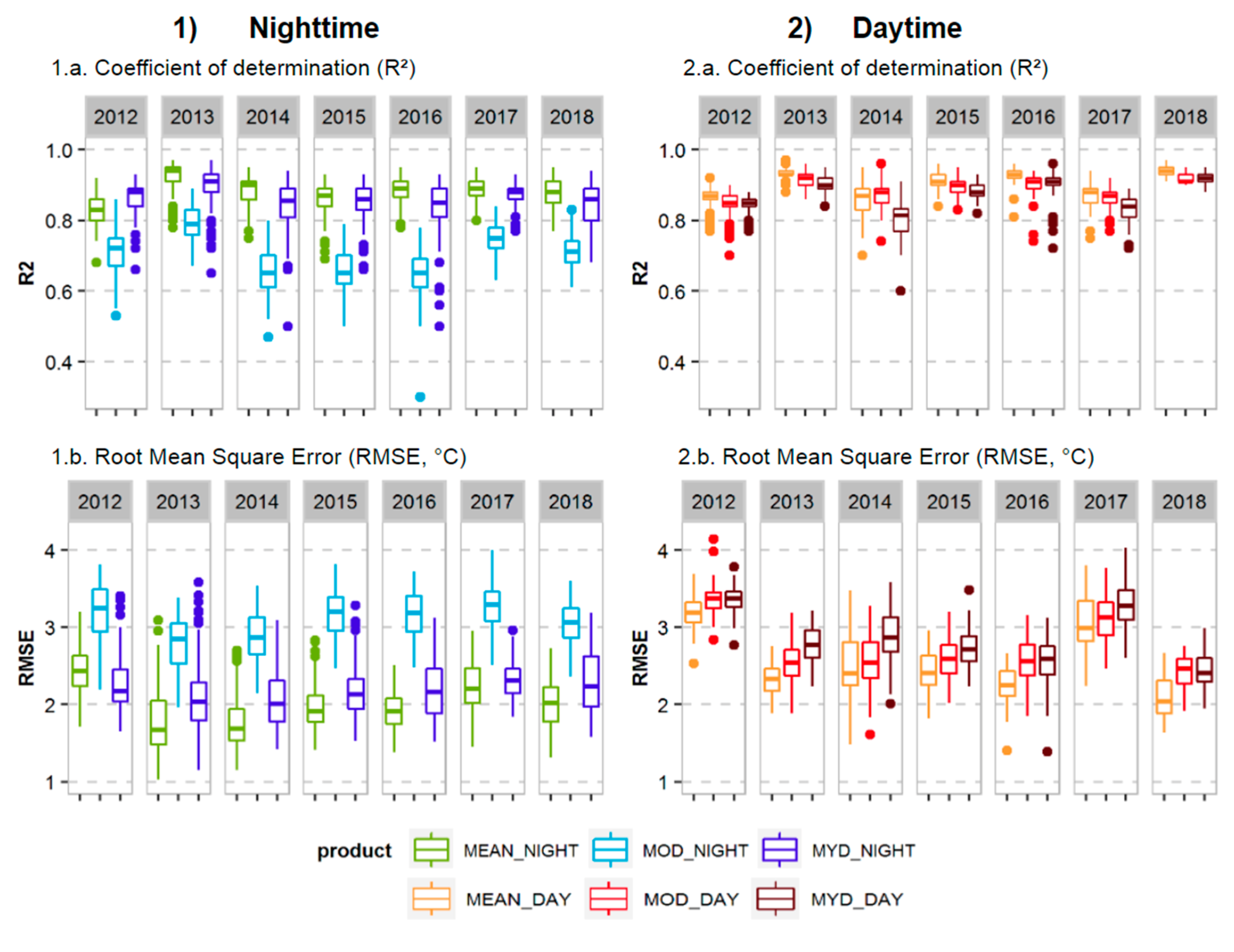
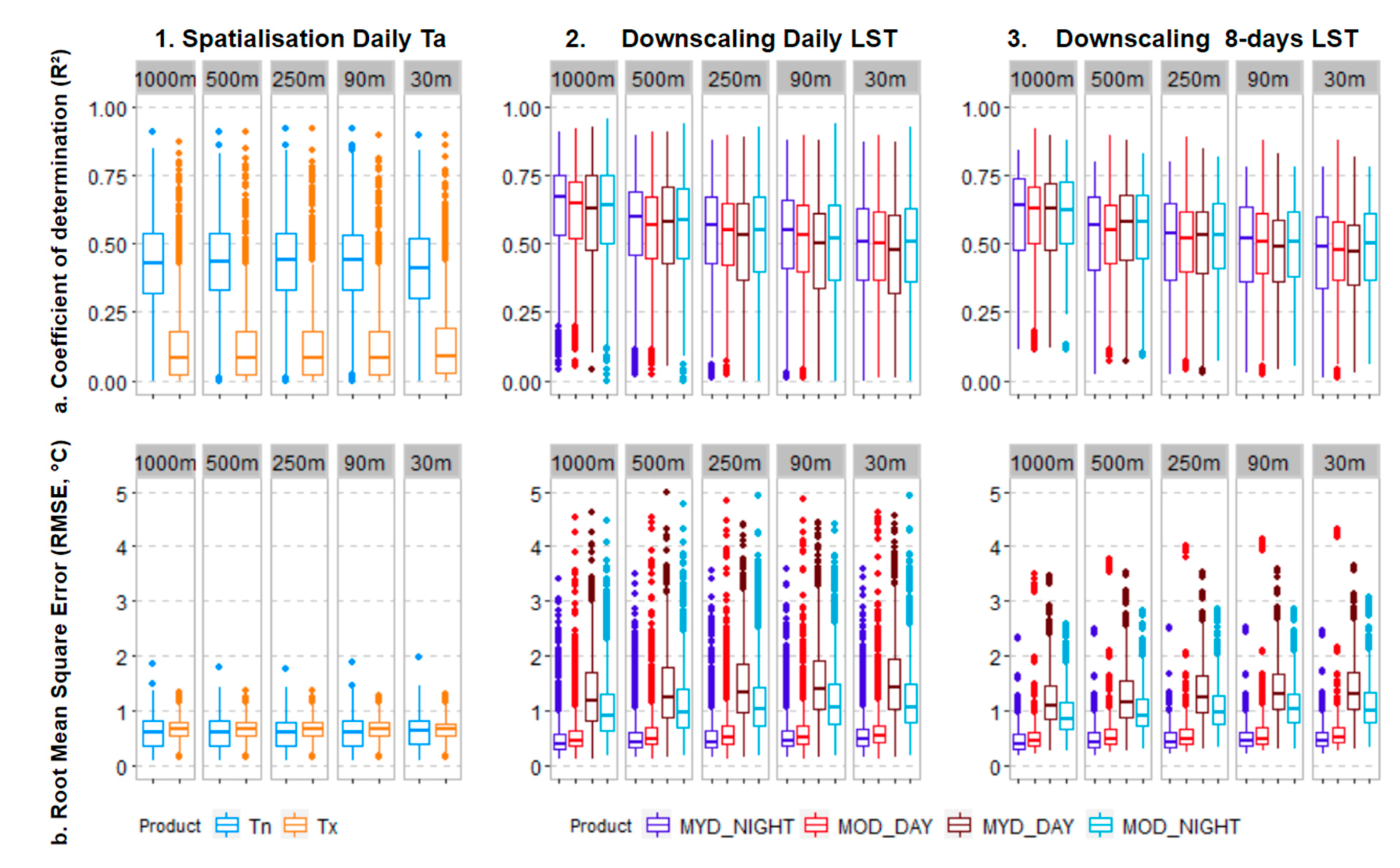
When calculating performances of daily SVM models for minimum air temperature (Tn) and maximum air temperature (Tx) time series and each MODIS product time series (MOD_DAY, MOD_NIGHT, MYD_DAY and MYD_NIGHT), the results varied greatly at all spatial resolutions (
Figure 6.1): R
2 of Tn and Tx ranged from 0.0-0.92, but the interquartile range of R
2 was 0.32–0.53 for Tn vs. 0.02–0.18 for Tx (
Figure 6.1a). For the daily LST (
Figure 6.2) and 8-day composite LST (
Figure 6.3), the interquartile ranges of R
2 were similar and ranged from 0.27–0.75. The RMSE was slightly better for lower resolutions (e.g., 1000 m) than higher resolutions (e.g., 30 m). For MODIS products, the MOD product (MOD_DAY and MOD_NIGHT) performed better than the MYD product (MYD_DAY and MYD_NIGHT). For the timing of acquisition, daytime products had slightly lower performance due to daytime atmospheric conditions. For nighttime acquisition, the MYD_NIGHT product had better performance and less variability than the MOD_NIGHT product. The downscaling performances between daily LST (M*D11A1,
Figure 6.2) and daily LST from weekly data (M*D11A2
Figure 6.3) were similar at all spatial resolutions. They differed mainly in RMSE, which had lower variability for the weekly products (M*D11A2,
Figure 6.3b). The downscaling method was less effective for air temperature than for LST.
The same statistical and evaluation methods were used to spatialize the air temperatures and downscale both types of LST data (daily and weekly). The performances of modeling air temperatures were lower than those of modeling the two types of LST. As continuous matrices of data, the remote sensing images cover the entire study area more accurately than point data from air temperature sensors.
3.2. Mapping Bioclimatic Indices Using Air Temperature and LST
The WI (
Figure 7) and HI (
Figure 8) bioclimatic indices at spatial resolutions of 30–1000 m and averaged for 2012–2018 demonstrated the influence of topographic variables used to spatialize temperatures. Index values calculated from air temperatures were lower than those calculated from LST. Topographic variables influenced greatly the indices calculated from air temperatures. The network of temperature sensors was installed to represent all topographic contexts of the study site. As a result, the variability in the microclimate was considered at a fine scale. In addition, for indices calculated from LST, the local topography was less visible in the downscaling, but thermal patterns were distinct and similar to those generated by air temperatures.
3.2.1. Spatial Distribution of Bioclimatic Indices
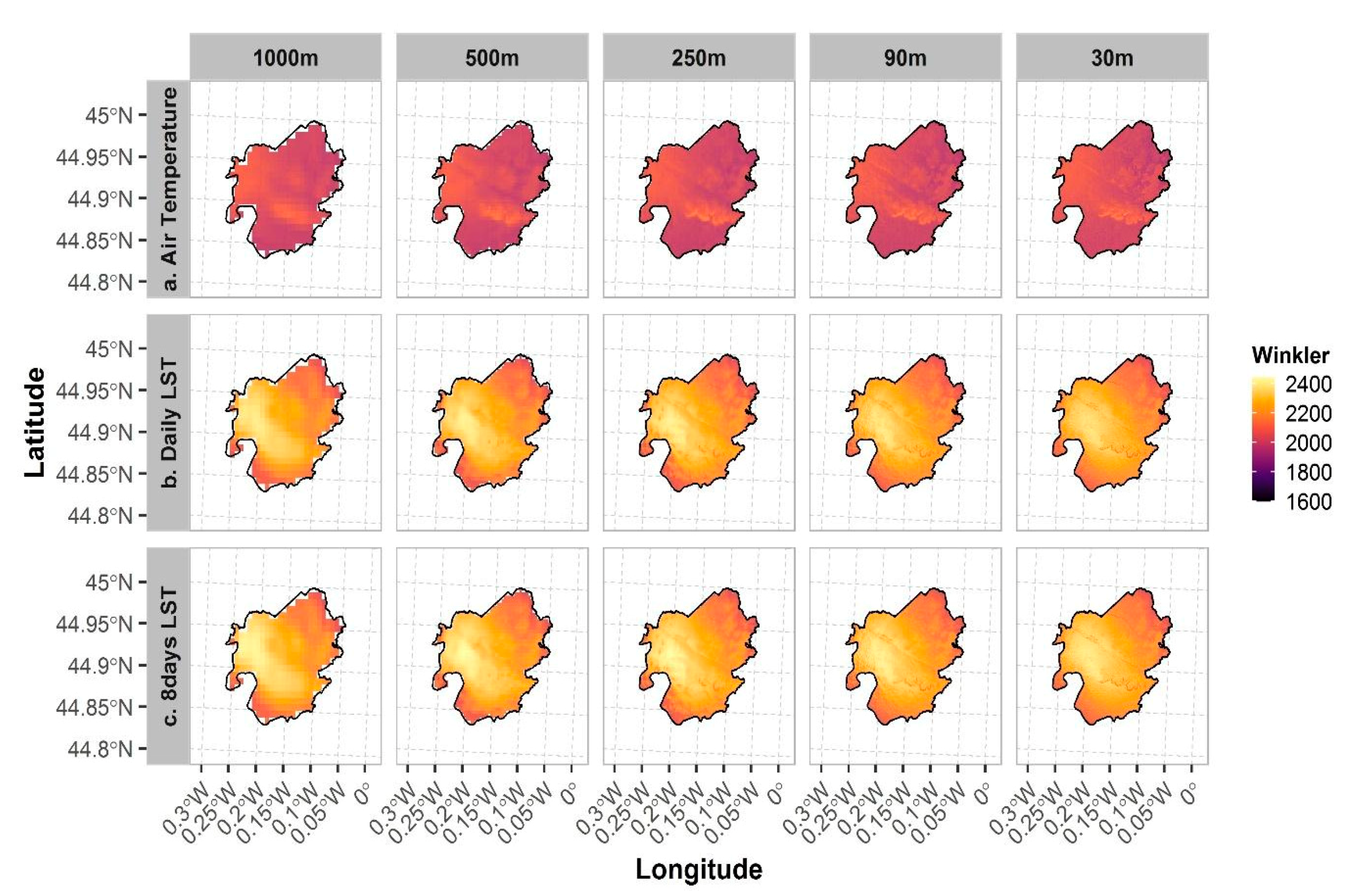
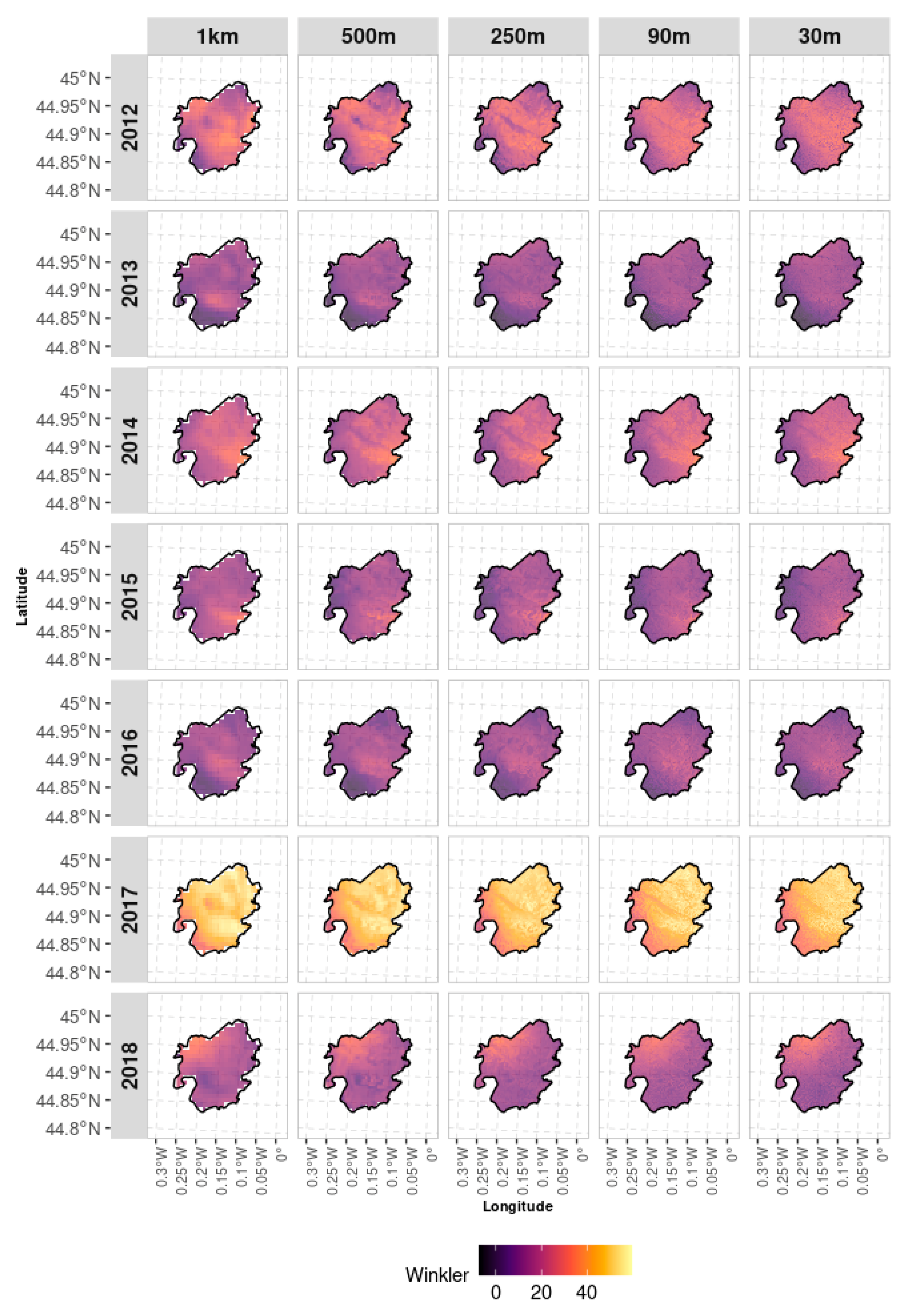
The WI averaged for 2012–2018 and over the study area calculated from air temperatures was 1840 °C (±1 standard deviation (SD) = 108 °C) (
Figure 7a). However, inter-annual variability was high, and several growing seasons were cooler than the average, with 1751 °C (2012), 1733 °C (2013), and 1751 °C (2016), and 2018 was the season with the highest WI (2036 °C). The WI increased as elevation increased, with marked differences among valley bottoms at the highest resolutions.
The WI calculated from the daily (M*D11A1,
Figure 7b) and weekly (M*D11A2,
Figure 7c) LST were similar and in the same order (from lowest to highest), but remained higher than those of the air temperatures. For these two LST datasets, WI of the 2013 season was much lower, and that of the 2018 season much higher, than the mean of the period and the other seasons individually. The highest WI appeared in the west of the study area, with a slight increase in areas with higher elevations, although less pronounced than the increase in air temperatures. The north and south of the study area had lower WI, like that for air temperatures.
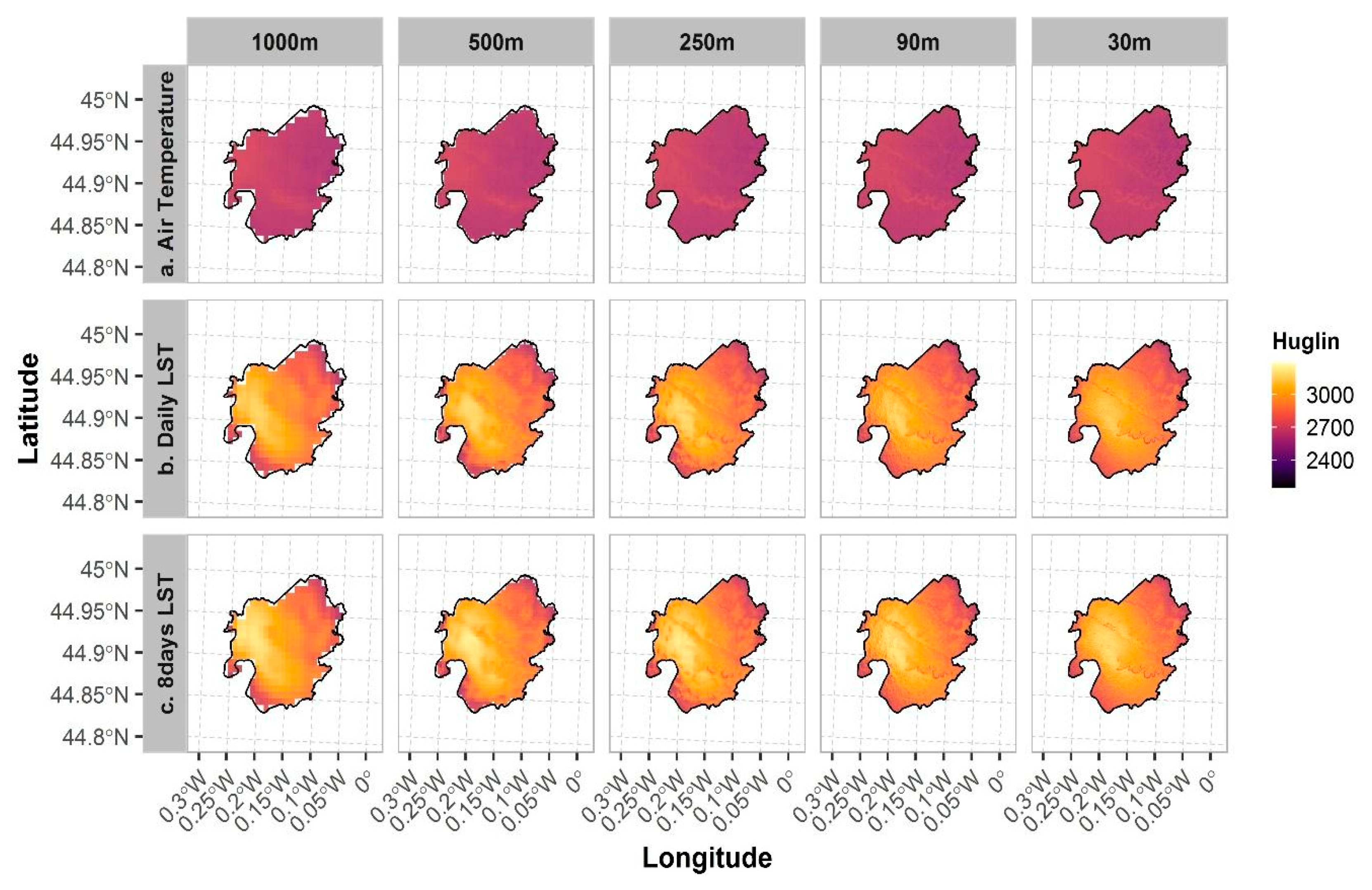
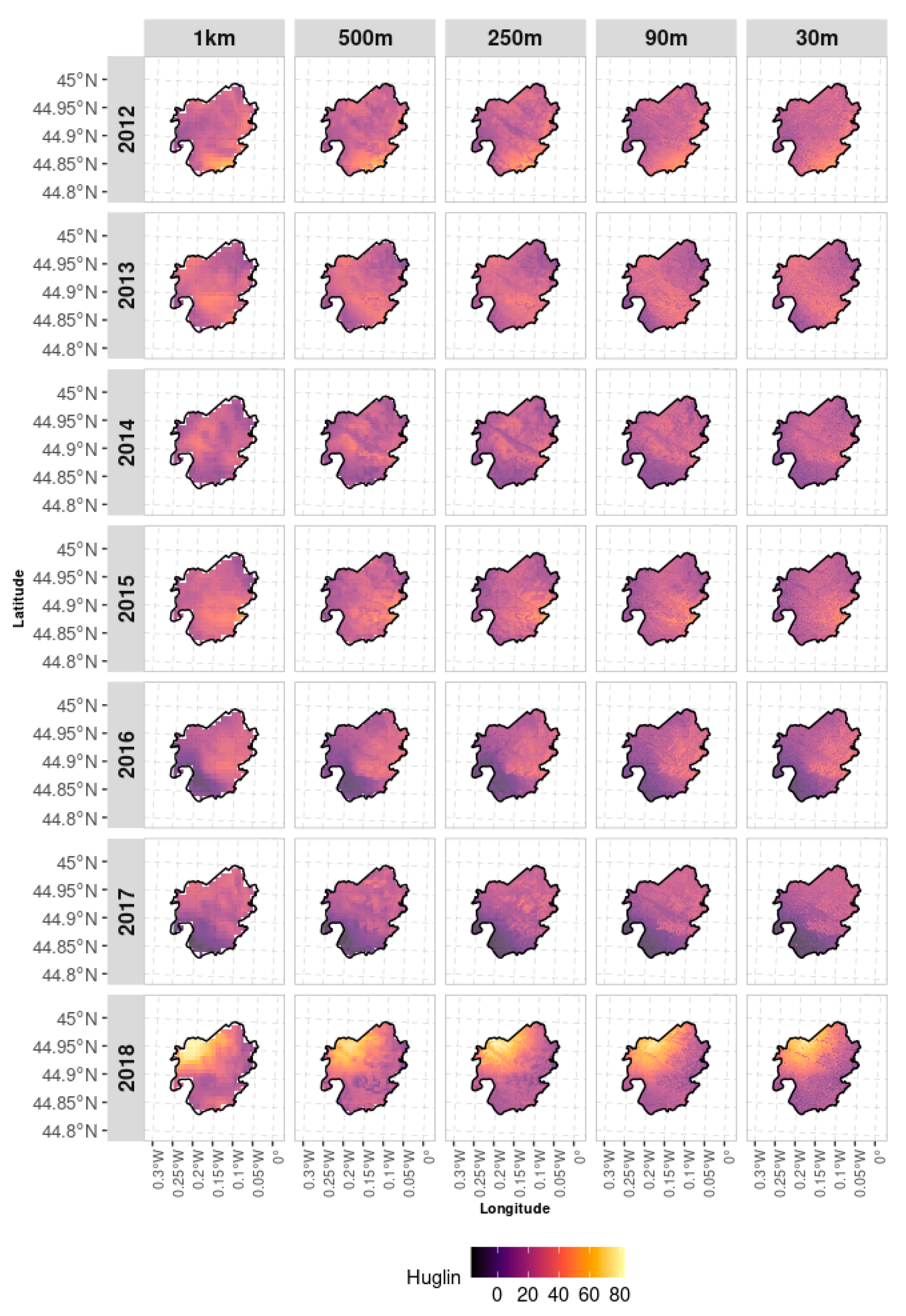
For the HI calculated from air temperature, the mean was 2410 °C (SD = 137 °C) averaged over the entire area for 2012–2018 and all resolutions (
Figure 8a). Regardless of the resolution, the maximum or minimum HI values were similar and spatially consistent. Variability was higher among growing seasons than among resolutions. At all resolutions of the study area, mean HI was lowest in the 2013 growing season (2209 °C) and highest in the 2018 growing season (2656 °C).
For daily (M*D11A1,
Figure 8a) and weekly (M*11A2,
Figure 8c) LST, the HI values were similar, with higher HI for the 8-day composite data. Thus, for 2012–2018 and all resolutions, mean HI was 2745 °C (SD = 209 °C) and 2768 °C (SD = 211 °C) for the daily LST and 8-day composite LST data, respectively. For air temperatures, the two HI calculated from LST reflected, for the given time series, lower HI for the 2014 growing season (daily: 2520 °C and 8-day: 2540 °C) and higher HI for the 2018 growing season (daily: 2939 °C and 8-day: 2971 °C). For air temperatures and LST, the inclusion of maximum temperatures in HI revealed a strong west/northeast gradient.
3.2.2. Evaluation of Difference between Air Temperature and LST Bioclimatic Indices
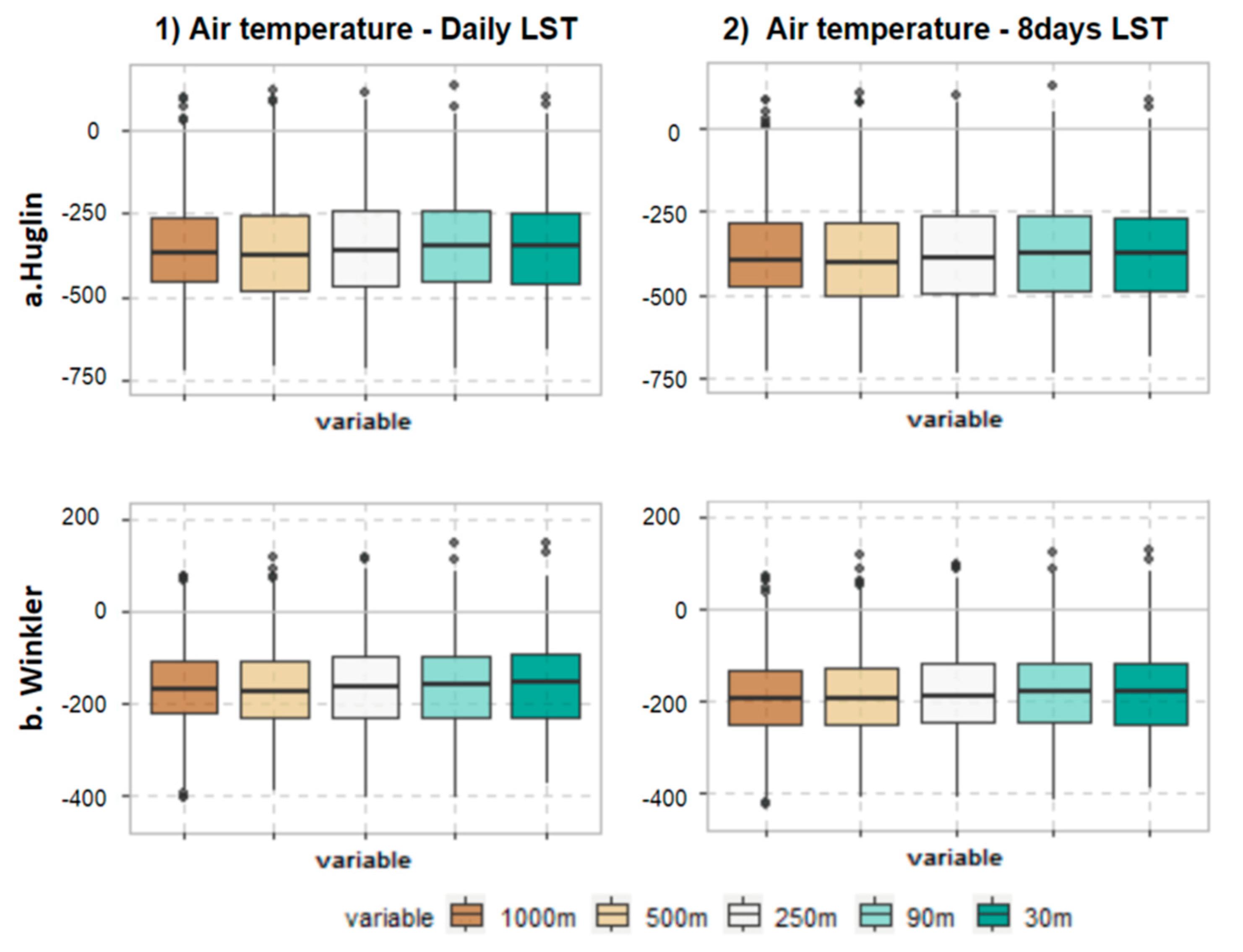
When calculating differences in the bioclimatic indices between air temperature and LST, LST tended to have higher values at all spatial resolutions (
Figure 9). For the WI (
Figure 9a), the differences and ranges of values were nearly the same at all resolutions. The difference in median WI was nearly 100 °C and that in interquartile ranges ranged from 0 °C to −150 °C. For the HI (
Figure 9b), the difference in the median was nearly 200 °C and that in the interquartile ranged from −100 °C for the first quartile to −300 °C for the third quartile. In addition to these results, correlations between bioclimatic indices based on air temperature and LST were calculated (
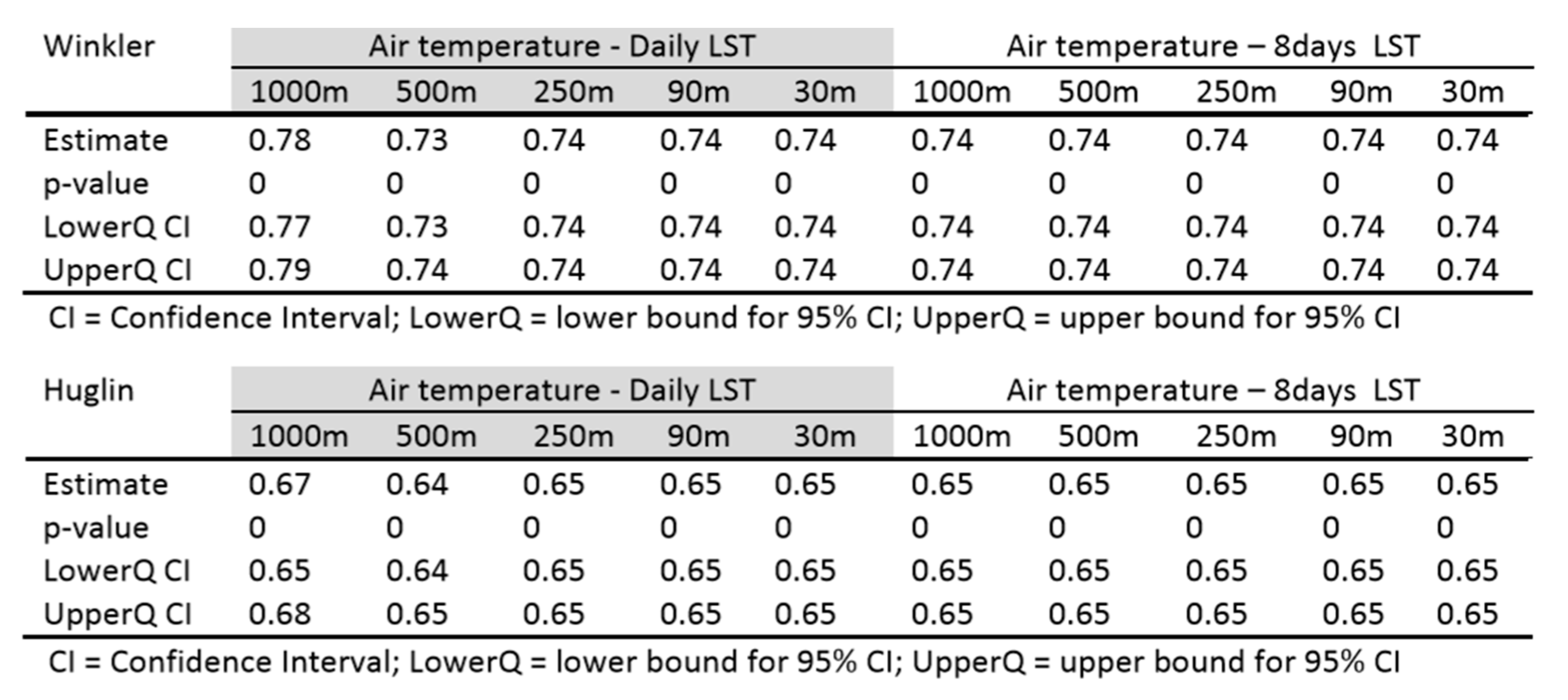
Appendix B,
Figure A3). Bioclimatic indices calculated from air temperature or calculated from LST had a higher positive Pearson correlation for the WI than for the HI, both for the daily and weekly LST correlated with air temperatures. All
p-values were under the significance level of 0.05, indicating that the Pearson correlation coefficients were statistically significant.
Differences in bioclimatic index values between (1) daily air temperature and daily LST and (2) daily air temperature and weekly LST were consistent at different spatial resolutions. The HI had higher variability in the differences than the WI, which gave weight to the maximum temperatures and generated more bias. In addition, the topography of the study site generated biases with larger differences, especially in areas with higher elevation and relief (
Appendix A,
Figure A1 and
Figure A2). Certain growing seasons were more distinct than others, such as the 2018 season for both indices (
Appendix A,
Figure A1 and
Figure A2), when the northwest of the study site had larger differences, or the 2017 season for the WI (
Appendix A,
Figure A1), which had the largest differences.
4. Discussion
The relationship between air temperature and grapevine development has been extensively studied and demonstrated across many winegrowing regions. The point data in the present study enabled us to analyze the thermal microclimate of grapevines, but they remain strongly limited in time and space. The thermal satellite data, despite representing the surface temperature above grapevines, appears to have potential in the search for more global coverage and the use of time series. This study demonstrated statistical relationships between daily air temperature and daily and weekly LST for nighttime (minimum) and daytime (maximum) data.
The main objective of this study was to evaluate the potential of the SVM approach to downscale LST bioclimatic indices in vineyards. The results of the daily and weekly 1000 m MODIS time-series downscaling at multiple spatial resolutions are encouraging for application to viticulture. The overall downscaling results using an SVM approach at all resolutions combined had R2 of 0.40–0.65 and RMSE of 0.4–1.6 °C, with more variable RMSE in daytime than in nighttime.
The lowest resolution (1000 m) is not suitable for monitoring cumulative temperatures because it does not consider topographic variables. The highest resolutions (30 and 90 m) seem better adapted to study local variability but generated biases that were too large because the topographic variables had a strong influence, and the models were oversampled. However, moderate resolutions, such as 500 or 250 m, provided more accurate information by decreasing the biases and errors associated with each step of the study. Moreover, the calculation times and smaller amount of data are reasonable for these two resolutions, which facilitates reproducibility.
The weekly data include less temperature variability than the daily data, but the results are still acceptable. By considering the biases, this approach can model the temperatures and indices with a spatial resolution suitable for the winegrowers (i.e., considering the terroir as much as possible). The objective was to evaluate the potential of MODIS thermal satellite imagery to calculate bioclimatic indices specific to viticulture by downscaling topographic variables. Daily and weekly LST in this approach are relevant to the scale of the grapevine growing season.
5. Conclusions
This study assessed LST downscaling to map bioclimatic indices in vineyards. Daily SVM models were applied based on the relationship between temperature and topographic variables. The approach demonstrated that SVM machine-learning regression was able to model daily temperatures accurately to calculate bioclimatic indices. The performance of LST is encouraging, but differs slightly from modeling air temperature. These differences and biases have been identified, but we have been investigating the spatial distribution between air temperatures from sensors network and the two MODIS (daily and weekly) LST. Downscaling LST at the scale of this type of site requires wider coverage and new topographic and vegetation variables to improve model training and validation. This study is an initial step in using LST to model the climate for viticulture, and in increasingly precise research of the true thermal microclimate of grapevines in a local environment, which may accentuate these effects or climatic events. This downscaling approach based on MODIS thermal satellite imagery is currently applied throughout the Gironde department, with validation from the national network of weather stations (LACCAVE2.21, IRP VINADAPT and AVVENIR projects).
Author Contributions
Conceptualization, G.M., R.L.R. and H.Q.; methodology, G.M.; software, G.M., P.-G.L. and R.L.R.; validation, G.M.; formal analysis, G.M., R.L.R., P.-G.L. and H.Q.; data curation, G.M., P.-G.L. and H.Q.; writing—original draft preparation, G.M.; supervision, H.Q.; project administration, H.Q. All authors have read and agreed to the published version of the manuscript.
Funding
This research was funded by the Conseil Interprofessionnel du Vin de Bordeaux (CIVB) and the AVVENIR project, grant number 51640/180008/9/10. The APC was funded by the metaprogramme Adaptation of Agriculture and Forests to Climate Change (AAFCC) of the French National Institute for Agriculture, Food and Environment Research (INRAE), especially through the Laccave2.21 project. This work was also supported by the IRP VINADAPT project.
Data Availability Statement
Not applicable.
Conflicts of Interest
The authors declare no conflict of interest. The funders had no role in the design of the study; in the collection, analyses, or interpretation of data; in the writing of the manuscript, or in the decision to publish the results.
Appendix A
Figure A1.
Spatial distribution of differences in the Winkler bioclimatic index calculated from daily land surface temperature (M*11A1) minus that calculated from the 8-day land surface temperature (M*D11A2) from 2012–2018 and gridded at different spatial resolutions.
Figure A1.
Spatial distribution of differences in the Winkler bioclimatic index calculated from daily land surface temperature (M*11A1) minus that calculated from the 8-day land surface temperature (M*D11A2) from 2012–2018 and gridded at different spatial resolutions.
Figure A2.
Spatial distribution of differences in the Huglin bioclimatic index calculated from daily land surface temperature (M*11A1) minus that calculated from the 8-day land surface temperature (M*D11A2) from 2012–2018 and gridded at different spatial resolutions.
Figure A2.
Spatial distribution of differences in the Huglin bioclimatic index calculated from daily land surface temperature (M*11A1) minus that calculated from the 8-day land surface temperature (M*D11A2) from 2012–2018 and gridded at different spatial resolutions.
Appendix B
Figure A3.
Table of Pearson correlation coefficients, computed between bioclimatic indices values from air temperature and LST, and statistical significance of the associated F-test.
Figure A3.
Table of Pearson correlation coefficients, computed between bioclimatic indices values from air temperature and LST, and statistical significance of the associated F-test.
References
- Van Leeuwen, C.; Seguin, G. The concept of terroir in viticulture. J. Wine Res. 2006, 17, 1–10. [Google Scholar] [CrossRef]
- Gladstones, J. Viticulture and Environment; Winetitles: Broadview, Australia, 1992. [Google Scholar]
- Jones, G.V.; Alves, F. Impact of climate change on wine production: A global overview and regional assessment in the Douro Valley of Portugal. Int. J. Glob. Warm. 2012, 4, 383–406. [Google Scholar] [CrossRef]
- Mira de Orduña, R. Climate change associated effects on grape and wine quality and production. Food Res. Int. 2010, 43, 1844–1855. [Google Scholar] [CrossRef]
- Winkler, A.J. Development and composition of grapes. Gen. Vitic. 1974, 138–196. [Google Scholar]
- Huglin, M.P. Nouveau mode d’evaluation des possibilites heliothermiques d’un milieu viticole. Comptes Rendus l’Académie d’Agric. Fr. 1978, 64, 1117–1126. [Google Scholar]
- Jones, G.; Moriondo, M.; Bois, B.; Hall, A.; Duff, A. Analysis of the spatial climate structure in viticulture regions worldwide. Bull. OIV 2009, 82, 507–517. [Google Scholar]
- Parker, A.K.; Cortázar-Atauri, I.G.D.; Leeuwen, C.V.; Chuine, I. General phenological model to characterise the timing of flowering and veraison of Vitis vinifera L. Aust. J. Grape Wine Res. 2011, 17, 206–216. [Google Scholar] [CrossRef]
- Ashcroft, M.B.; Gollan, J.R. Fine-resolution (25 m) topoclimatic grids of near-surface (5 cm) extreme temperatures and humidities across various habitats in a large (200 × 300 km) and diverse region. Int. J. Climatol. 2012, 32, 2134–2148. [Google Scholar] [CrossRef]
- Scherrer, D.; Körner, C. Topographically controlled thermal-habitat differentiation buffers alpine plant diversity against climate warming. J. Biogeogr. 2011, 38, 406–416. [Google Scholar] [CrossRef]
- Quénol, H. Viticulture—Experimentation or adaptation? In Adaptating to Climate Change; Thiebault, S., Laville, B., Euzen, A., Eds.; EdiSens: Isle Royale National Park, MI, USA, 2017; pp. 333–340. [Google Scholar]
- Fraga, H.; de Cortázar Atauri, I.G.; Malheiro, A.C.; Santos, J.A. Modelling climate change impacts on viticultural yield, phenology and stress conditions in Europe. Glob. Change Biol. 2016, 22, 3774–3788. [Google Scholar] [CrossRef]
- Le Roux, R.; De Rességuier, L.; Katurji, M.; Zawar-Reza, P.; Sturman, A.; Van Leeuwen, C.; Quénol, H. Analyse multiscalaire de la variabilité spatiale et temporelle des températures à l’échelle des appellations viticoles de Saint-Émilion, Pomerol et leurs satellites. Climatologie 2017. [Google Scholar] [CrossRef]
- Quénol, H.; de Cortazar Atauri, I.G.; Bois, B.; Sturman, A.; Bonnardot, V.; Roux, R.L. Which climatic modeling to assess climate change impacts on vineyards? OENO One 2017, 51, 91–97. [Google Scholar] [CrossRef]
- Sturman, A.; Zawar-Reza, P.; Soltanzadeh, I.; Katurji, M.; Bonnardot, V.; Parker, A.K.; Trought, M.C.T.; Quénol, H.; Roux, R.L.; Gendig, E.; et al. The application of high-resolution atmospheric modelling to weather and climate variability in vineyard regions. OENO One 2017, 51, 99–105. [Google Scholar] [CrossRef]
- van Leeuwen, C.; Roby, J.P.; Pernet, D.; Bois, B. Methodology of soil-based zoning for viticultural terroirs. Bull. OIV 2010, 83, 13–29. [Google Scholar]
- Zorer, R.; Rocchini, D.; Metz, M.; Delucchi, L.; Zottele, F.; Meggio, F.; Neteler, M. Daily MODIS Land Surface Temperature Data for the Analysis of the Heat Requirements of Grapevine Varieties. IEEE Trans. Geosci. Remote Sens. 2013, 51, 2128–2135. [Google Scholar] [CrossRef]
- Hutengs, C.; Vohland, M. Downscaling land surface temperatures at regional scales with random forest regression. Remote Sens. Environ. 2016, 178, 127–141. [Google Scholar] [CrossRef]
- Wang, Q.; Rodriguez-Galiano, V.; Atkinson, P.M. Geostatistical Solutions for Downscaling Remotely Sensed Land Surface Temperature. ISPRS Int. Arch. Photogramm. Remote Sens. Spat. Inf. Sci. 2017, 42W7, 913–917. [Google Scholar] [CrossRef]
- Yang, Y.; Li, X.; Pan, X.; Zhang, Y.; Cao, C.; Yang, Y.; Li, X.; Pan, X.; Zhang, Y.; Cao, C. Downscaling Land Surface Temperature in Complex Regions by Using Multiple Scale Factors with Adaptive Thresholds. Sensors 2017, 17, 744. [Google Scholar] [CrossRef]
- Bartkowiak, P.; Castelli, M.; Notarnicola, C. Downscaling land surface temperature from MODIS dataset with random forest approach over alpine vegetated areas. Remote Sens. 2019, 11, 1319. [Google Scholar] [CrossRef]
- Huang, R.; Zhang, C.; Huang, J.; Zhu, D.; Wang, L.; Liu, J. Mapping of Daily Mean Air Temperature in Agricultural Regions Using Daytime and Nighttime Land Surface Temperatures Derived from TERRA and AQUA MODIS Data. Remote Sens. 2015, 7, 8728–8756. [Google Scholar] [CrossRef]
- Shi, L.; Liu, P.; Kloog, I.; Lee, M.; Kosheleva, A.; Schwartz, J. Estimating daily air temperature across the Southeastern United States using high-resolution satellite data: A statistical modeling study. Environ. Res. 2016, 146, 51–58. [Google Scholar] [CrossRef] [PubMed]
- Meyer, H.; Katurji, M.; Appelhans, T.; Müller, M.; Nauss, T.; Roudier, P.; Zawar-Reza, P. Mapping Daily Air Temperature for Antarctica Based on MODIS LST. Remote Sens. 2016, 8, 732. [Google Scholar] [CrossRef]
- Zhou, W.; Peng, B.; Shi, J.; Wang, T.; Dhital, Y.; Yao, R.; Yu, Y.; Lei, Z.; Zhao, R.; Zhou, W.; et al. Estimating High Resolution Daily Air Temperature Based on Remote Sensing Products and Climate Reanalysis Datasets over Glacierized Basins: A Case Study in the Langtang Valley, Nepal. Remote Sens. 2017, 9, 959. [Google Scholar] [CrossRef]
- Xu, Y.; Knudby, A.; Shen, Y.; Liu, Y. Mapping monthly air temperature in the Tibetan Plateau from MODIS data based on machine learning methods. IEEE J. Sel. Top. Appl. Earth Obs. Remote Sens. 2018, 11, 345–354. [Google Scholar] [CrossRef]
- Morin, G.; Le Roux, R.; Sturman, A.; Quénol, H. Évaluation de la relation entre températures de l’air et températures de surface issues du satellite MODIS: Application aux vignobles de la vallée de Waipara (Nouvelle-Zélande). Climatologie 2018, 15, 62–83. [Google Scholar] [CrossRef]
- Wan, Z. New refinements and validation of the MODIS Land-Surface Temperature/Emissivity products. Remote Sens. Environ. 2008, 112, 59–74. [Google Scholar] [CrossRef]
- Bechtel, B.; Zakšek, K.; Hoshyaripour, G. Downscaling Land Surface Temperature in an Urban Area: A Case Study for Hamburg, Germany. Remote Sens. 2012, 4, 3184–3200. [Google Scholar] [CrossRef]
- Zakšek, K.; Oštir, K. Downscaling land surface temperature for urban heat island diurnal cycle analysis. Remote Sens. Environ. 2012, 117, 114–124. [Google Scholar] [CrossRef]
- Zhan, W.; Chen, Y.; Zhou, J.; Wang, J.; Liu, W.; Voogt, J.; Zhu, X.; Quan, J.; Li, J. Disaggregation of remotely sensed land surface temperature: Literature survey, taxonomy, issues, and caveats. Remote Sens. Environ. 2013, 131, 119–139. [Google Scholar] [CrossRef]
- Zhou, J.; Jia, L.; Menenti, M.; Gorte, B. On the performance of remote sensing time series reconstruction methods – A spatial comparison. Remote Sens. Environ. 2016, 187, 367–384. [Google Scholar] [CrossRef]
- Ebrahimy, H.; Azadbakht, M. Downscaling MODIS land surface temperature over a heterogeneous area: An investigation of machine learning techniques, feature selection, and impacts of mixed pixels. Comput. Geosci. 2019, 124, 93–102. [Google Scholar] [CrossRef]
- Kottek, M.; Grieser, J.; Beck, C.; Rudolf, B.; Rubel, F. World Map of the Köppen-Geiger climate classification updated. Meteorol. Z. 2006, 15, 259–263. [Google Scholar] [CrossRef]
- Quénol, H. Changement climatique et Terroirs Viticoles; Lavoisier Tec&Doc: Paris, France, 2014; ISBN 978-2-7430-1575-6. [Google Scholar]
- van Leeuwen, C.; Darriet, P. The Impact of Climate Change on Viticulture and Wine Quality*. J. Wine Econ. 2016, 11, 150–167. [Google Scholar] [CrossRef]
- van Leeuwen, C.; Destrac-Irvine, A. Modified grape composition under climate change conditions requires adaptations in the vineyard. OENO One 2017, 51, 147–154. [Google Scholar] [CrossRef]
- Le Roux, R.; de Rességuier, L.; Corpetti, T.; Jégou, N.; Madelin, M.; van Leeuwen, C.; Quénol, H. Comparison of two fine scale spatial models for mapping temperatures inside winegrowing areas. Agric. For. Meteorol. 2017, 247, 159–169. [Google Scholar] [CrossRef]
- Farr, T.G.; Rosen, P.A.; Caro, E.; Crippen, R.; Duren, R.; Hensley, S.; Kobrick, M.; Paller, M.; Rodriguez, E.; Roth, L. The shuttle radar topography mission. Rev. Geophys. 2007, 45. [Google Scholar] [CrossRef]
- Danielson, J.J.; Gesch, D.B. Global Multi-Resolution Terrain Elevation Data 2010 (GMTED2010); US Department of the Interior, US Geological Survey: Washington, DC, USA, 2011.
- De Rességuier, L.; Mary, S.; Le Roux, R.; Petitjean, T.; Quénol, H.; van Leeuwen, C. Temperature variability at local scale in the Bordeaux area. Relations with environmental factors and impact on vine phenology. Front. Plant Sci. 2020, 11, 515. [Google Scholar] [CrossRef]
- Parker, A.; de Cortázar-Atauri, I.G.; Chuine, I.; Barbeau, G.; Bois, B.; Boursiquot, J.-M.; Cahurel, J.-Y.; Claverie, M.; Dufourcq, T.; Gény, L.; et al. Classification of varieties for their timing of flowering and veraison using a modelling approach: A case study for the grapevine species Vitis vinifera L. Agric. For. Meteorol. 2013, 180, 249–264. [Google Scholar] [CrossRef]
- Wan, Z.; Hook, S.; Hulley, G. MOD11A2 MODIS/Terra Land Surface Temperature/Emissivity 8-Day L3 Global 1km SIN Grid V006; NASA EOSDIS Land Processes DAAC: Sioux Falls, SD, USA, 2015; Volume 10. [Google Scholar]
- Wan, Z.; Hook, S.; Hulley, G. MOD11A1 MODIS/Terra Land Surface Temperature/Emissivity Daily L3 Global 1 km SIN Grid V006 [Data Set]; NASA EOSDIS Land Processes DAAC: Sioux Falls, SD, USA, 2015; Volume 10. [Google Scholar]
- Cortes, C.; Vapnik, V. Support-vector networks. Mach. Learn. 1995, 20, 273–297. [Google Scholar] [CrossRef]
- Kuhn, M. The Caret Package. R Found. Stat. Comput. Vienna Austria URL Httpscran R-Proj. Orgpackage Caret 2012. Available online: https://cran.r-project.org/web/packages/caret/caret.pdf (accessed on 21 December 2020).
- Meyer, D.; Dimitriadou, E.; Hornik, K.; Weingessel, A.; Leisch, F.; Chang, C.C.; Lin, C.C. e1071: Misc functions of the Department of Statistics (e1071), TU Wien. R Package Version 2014, 1. Available online: https://cran.r-project.org/web/packages/e1071/e1071.pdf (accessed on 21 December 2020).
- Le Roux, R. Modélisation Climatique à l’échelle des Terroirs Viticoles dans un Contexte de Changement Climatique. Ph.D. Thesis, Université Rennes 2, Rennes, France, 2017. [Google Scholar]
- Amerine, M.; Winkler, A. Composition and Quality of Musts and Wines of California Grapes. Hilgardia 1944, 15, 493–675. [Google Scholar] [CrossRef]
- Mostovoy, G.V.; King, R.L.; Reddy, K.R.; Kakani, V.G.; Filippova, M.G. Statistical Estimation of Daily Maximum and Minimum Air Temperatures from MODIS LST Data over the State of Mississippi. GIScience Remote Sens. 2006, 43, 78–110. [Google Scholar] [CrossRef]
- Zhang, L.; Huang, J.; Guo, R.; Li, X.; Sun, W.; Wang, X. Spatio-temporal reconstruction of air temperature maps and their application to estimate rice growing season heat accumulation using multi-temporal MODIS data. J. Zhejiang Univ. Sci. B 2013, 14, 144–161. [Google Scholar] [CrossRef] [PubMed]
- Noi, P.; Kappas, M.; Degener, J. Estimating Daily Maximum and Minimum Land Air Surface Temperature Using MODIS Land Surface Temperature Data and Ground Truth Data in Northern Vietnam. Remote Sens. 2016, 8, 1002. [Google Scholar] [CrossRef]
- Benali, A.; Carvalho, A.C.; Nunes, J.P.; Carvalhais, N.; Santos, A. Estimating air surface temperature in Portugal using MODIS LST data. Remote Sens. Environ. 2012, 124, 108–121. [Google Scholar] [CrossRef]
- Sun, L.; Chen, Z.; Gao, F.; Anderson, M.; Song, L.; Wang, L.; Hu, B.; Yang, Y. Reconstructing daily clear-sky land surface temperature for cloudy regions from MODIS data. Comput. Geosci. 2017, 105, 10–20. [Google Scholar] [CrossRef]
- Zeng, L.; Wardlow, B.D.; Tadesse, T.; Shan, J.; Hayes, M.J.; Li, D.; Xiang, D. Estimation of daily air temperature based on MODIS land surface temperature products over the corn belt in the US. Remote Sens. 2015, 7, 951–970. [Google Scholar] [CrossRef]
Figure 1.
(a,b) The Saint-Emilion and Pomerol study site (red border) and the administrative department of Gironde (black border) in southwestern France, and (c) the study site’s topography and network of 90 air temperature data loggers (black points).
Figure 1.
(a,b) The Saint-Emilion and Pomerol study site (red border) and the administrative department of Gironde (black border) in southwestern France, and (c) the study site’s topography and network of 90 air temperature data loggers (black points).
Figure 2.
Chronology of acquisition of air temperature (sensors) and land surface temperature (LST) (Terra (MOD) and Aqua (MYD) satellites for (N)ighttime and (D)aytime. Blue arrows indicate calculation intervals of mean daily minimum air temperature (Tn) and LST (LSTn), while red arrows indicate those of mean daily maximum air temperature (Tx) and LST (LSTx).
Figure 3.
Flowchart of the general method used for data: air temperature (Ta), daily land surface temperature (LST) (MOD11A1/MYD11A1), weekly LST (MOD11A2/MYD11A2) and multiple resolutions of digital elevation models. (A) Times series reconstruction, (B) Data description, (C) Spatialization of air temperature and downscaling of LST, (D) Calculation of bioclimatic indices for the growing season.
Figure 4.
Boxplots of statistical indicators of the linear relationship between daily air temperature and daily land surface temperature (M*D11A1) from 2012–2018 gridded at different spatial resolutions, by the type of MODIS product for each year studied: (a) coefficient of determination (R2) and (b) root mean square error (RMSE).
Figure 5.
Boxplots of statistical indicators of the linear relationship between daily air temperature and daily land surface temperature derived from an 8-day composite (M*D11A2) from 2012–2018 gridded at different spatial resolutions, by the type of MODIS product for each year studied: (a) coefficient of determination (R2) and (b) root mean square error (RMSE).
Figure 6.
Boxplots of statistical indicators of the downscaling of (1) spatialization of air temperature, (2) downscaling of daily land surface temperature (LST) and (3) downscaling of the 8-day composite LST using the support vector machine algorithm gridded at different spatial resolutions, by the type of product for each year studied: (a) coefficient of determination (R2) and (b) root mean square error (RMSE, in °C).
Figure 7.
Spatial distribution of the Winkler index averaged from 2012–2018 and gridded at different spatial resolutions using (a) predicted air temperature, (b) downscaled daily land surface temperature (LST) (M*D11A1) and (c) downscaled 8-day LST (M*D11A2).
Figure 7.
Spatial distribution of the Winkler index averaged from 2012–2018 and gridded at different spatial resolutions using (a) predicted air temperature, (b) downscaled daily land surface temperature (LST) (M*D11A1) and (c) downscaled 8-day LST (M*D11A2).
Figure 8.
Spatial distribution of the Huglin index averaged from 2012–2018 and gridded at different spatial resolutions using (a) predicted air temperature, (b) downscaled daily land surface temperature (LST) (M*D11A1) and (c) downscaled 8-day LST (M*D11A2).
Figure 8.
Spatial distribution of the Huglin index averaged from 2012–2018 and gridded at different spatial resolutions using (a) predicted air temperature, (b) downscaled daily land surface temperature (LST) (M*D11A1) and (c) downscaled 8-day LST (M*D11A2).
Figure 9.
Distribution of differences (°C) between (1) daily air temperature and daily LST and (2) daily air temperature and 8days LST using to calculate the (a) Huglin and (b) Winkler bioclimatic indices at different spatial resolutions.
Figure 9.
Distribution of differences (°C) between (1) daily air temperature and daily LST and (2) daily air temperature and 8days LST using to calculate the (a) Huglin and (b) Winkler bioclimatic indices at different spatial resolutions.
Table 1.
Overview of original dataset used in the study.
Table 1.
Overview of original dataset used in the study.
| Data | Product and Source | Spatial Resolution | Temporal Resolution | Variable |
|---|
| Digital elevation model | SRTM—NASA | 30 m | - | Elevation (m) |
| 90 m | - | Slope (°) |
| GMTED—USGS | 250 m | - | N-S orientation (°) |
| 500 m | - | E-W orientation (°) |
| 1000 m | - | Coordinates (Lat./Long.) |
| Air temperature | TinyTag network | point | hourly | Minimum (Tn) and maximum (Tx) air temperature (°C) |
| Land surface temperature | MOD11A1/
MYD11A1 | 1000 m | daily (2 nighttime, 2 daytime) | Minimum and maximum land surface temperature (°C) |
MOD11A2/
MYD11A2 | 1000 m | 8-day composite (2 nighttime, 2 daytime) | Minimum and maximum land surface temperature (°C) |
| Publisher’s Note: MDPI stays neutral with regard to jurisdictional claims in published maps and institutional affiliations. |
© 2020 by the authors. Licensee MDPI, Basel, Switzerland. This article is an open access article distributed under the terms and conditions of the Creative Commons Attribution (CC BY) license (http://creativecommons.org/licenses/by/4.0/).


