Imputing Satellite-Derived Aerosol Optical Depth Using a Multi-Resolution Spatial Model and Random Forest for PM_2.5 Prediction

Abstract

A task for environmental health research is to produce complete pollution exposure maps despite limited monitoring data. Satellite-derived aerosol optical depth (AOD) is frequently used as a predictor in various models to improve PM_2.5 estimation, despite significant gaps in coverage. We analyze PM_2.5 and AOD from July 2011 in the contiguous United States. We examine two methods to aid in gap-filling AOD: (1) lattice kriging, a spatial statistical method adapted to handle large amounts data, and (2) random forest, a tree-based machine learning method. First, we evaluate each model’s performance in the spatial prediction of AOD, and we additionally consider ensemble methods for combining the predictors. In order to accurately assess the predictive performance of these methods, we construct spatially clustered holdouts to mimic the observed patterns of missing data. Finally, we assess whether gap-filling AOD through one of the proposed ensemble methods can improve prediction of PM_2.5 in a random forest model. Our results suggest that ensemble methods of combining lattice kriging and random forest can improve AOD gap-filling. Based on summary metrics of performance, PM_2.5 predictions based on random forest models were largely similar regardless of the inclusion of gap-filled AOD, but there was some variability in daily model predictions.

1. Introduction

Ambient outdoor air pollution, particularly particulate matter less than 2.5 micrometers in aerodynamic diameter (PM_2.5), poses a substantial risk to human health [1,2,3]. Air pollution monitors that can directly measure pollution concentrations are placed at a limited set of locations, resulting in large areas without direct measurements of ground-level pollution exposure. Aerosol optical depth (AOD) measures the amount of aerosol in the atmosphere and can be remotely sensed by satellite instruments at various spatial resolutions [4]. A growing literature has developed for using satellite-derived AOD as a proxy and predictor for PM_2.5 concentrations, often in conjunction with land-use and meteorological variables, using a range of model types such as geographically weighted regression, linear mixed effect models, and machine learning methods [5,6,7].

However, AOD itself has substantial missingness, complicating the process of predicting PM_2.5 concentrations. Gaps in AOD coverage are a result of cloud cover, snow cover, and surface brightness; for the moderate resolution imaging spectroradiometer (MODIS) 10 km product, on average each grid cell has no AOD available on approximately 70% of days, with substantial variation across regions [8,9]. AOD’s patterns of missingness are also not random for the purpose of PM_2.5 prediction; cloud and snow cover may plausibly be related to PM_2.5 concentrations [9,10]. At the scale of the continental United States, research suggests that missingness as a result of cloud cover is not likely to greatly bias monthly and yearly PM_2.5, although there is regional and seasonal variation [11]. However, Liang et al. [12] show that long-term PM_2.5 estimates in China are substantially biased as result of missing AOD observations. Furthermore, for health effects research, the relevant geographic scale is small and more impacted by missingness. When using PM_2.5 estimates based on satellite-derived AOD with substantial missingness, time series studies will miss many days and lose statistical power, and cohort studies will use potentially biased exposure estimates, resulting in a loss of statistical power. A number of approaches have been proposed for handling missing AOD observations when estimating PM_2.5 [7]. One approach has been to combine different AOD retrievals, although this will still result in incomplete coverage; e.g., Geng et al. [13] combine AOD measurements from Terra and Aqua satellites using linear regression. Other approaches have used AOD where available, but otherwise bypassed the need for gap-filling AOD [14,15,16].

Many recent studies use multi-stage approaches, where AOD is gap-filled, and then a model relating PM_2.5 to the gap-filled AOD and other land-use and meteorological variables is fit. These gap-filling models may use land-use and meteorological terms, as well as chemical transport model (CTM) estimates. Hu et al. [17] forego a statistical modeling procedure for gap-filling AOD, saving computational time, and they replace missing AOD values with CTM (GEOS-Chem) estimates of AOD. Xiao et al. [18] and Huang et al. [19] use linear models that include cloud fraction estimates, meteorological and land-use data together with smoothing splines, to account for spatial correlation for imputing AOD. Lv et al. [20] gap-fill AOD using a model that relates AOD to the ratio of daily and seasonal averages of PM_2.5 multiplied by the average seasonal AOD values for the grid cell for each city under study; a second stage then uses ordinary Kriging to fill in the remaining gaps. Because of the computational costs of ordinary Kriging, this method will not scale well to large datasets, but previous studies suggest that smoothing splines may not perform as well as Kriging in some settings [21]. Chen et al. [22] use a mixed effect model to first combine Terra and Aqua AOD measurements, and interpolate missing AOD values using inverse-distance weighting (IDW). IDW with a maximum distance will not be able to provide full coverage for AOD, however, as there are large missing areas with no observed data. Random forest (RF) is a popular machine learning method used for gap-filling, due to the fast implementations available and its ability to account for complex non-linear interactions of features [7,23]. Bi et al. [10] uses a two-stage model with RF being used to impute AOD using a number of relevant variables, including MODIS cloud and snow fractions. Several other recent papers impute AOD as part of a multi-stage process using RF (e.g., see Stafoggia et al. [24], Huang et al. [25], and Zhang et al. [26]). However, judging performance based on “out-of-bag” measures or random holdouts of observed data may be misleading in spatial prediction problems with large contiguous areas of missing data. Furthermore, when a strong spatial pattern is present as in AOD, it is unclear how RF performs compared to spatial statistical models. Jiang et al. [27] use RF to gap-fill AOD in China and evaluate performance using aerosol robotic network (AERONET) measurements [28,29]; however, there are relatively few locations with AERONET measurements on which to validate performance on any given day.

Importantly, models for gap-filling AOD are generally more costly to fit than models for estimating PM_2.5, due to the much larger number of daily observations. For example, in our case study, using a modeling grid of 12 km spatial resolution over the contiguous United States entails over 50,000 daily cells. While several studies have used machine learning methods for AOD gap-filling to overcome the computational costs, traditional spatial statistical methods like Kriging are not well-suited to handle large datasets due to the need to invert the spatial covariance matrix. Over the course of the last decade or so, several spatial statistical methods have been developed to handle big data [30,31]. Although considerable attention has been given to using ensemble and hybrid approaches for estimating PM_2.5 (e.g., [32,33,34,35]), AOD gap-filling for large areas has received less focus, possibly due to the greater computational cost.

To our knowledge, studies have not thus far considered ensemble methods for combining large-scale spatial statistical methods with machine learning methods for gap-filling AOD. In this study, we focus on a particular spatial statistical method, lattice kriging (LK) [36], together with RF for AOD gap-filling. Our study considers both RF and LK models for gap-filling MODIS AOD, as well as ensemble methods for combining these predictions following the super learner methodology [37,38]. Our case study focuses on the contiguous United States using daily data for the month of July 2011. We focus on a single month for computational reasons as each AOD model is fit daily to tens of thousands of observations, and we perform 10-fold cross-validation on each day as part of the ensemble method construction, resulting in an additional 10 models fit per day for LK and RF. We assess performance using spatially clustered holdouts for AOD gap-filling models that may more accurately measure performance than more commonly used approaches. Finally, we assess whether the imputed AOD product using ensemble methods improves PM_2.5 estimation in a random forest model. Broadly, we find that ensemble methods can be effective for AOD gap-filling, but there is less evidence to suggest an ultimate benefit for PM_2.5 estimation.

2. Materials and Methods

2.1. Study Area

The study area of interest is the contiguous United States, consisting of 48 states, and Washington DC, using daily data for the month of July 2011. We focused our analysis on July, as summer months generally have less AOD missingness than other months on average, while retaining substantial day-to-day variability in missingness. Descriptions of the data sources follow the work of Hu et al. [17].

2.2. PM_2.5 Measurements

We obtain measurements of PM_2.5 from the U.S. Environmental Protection Agency (EPA) Air Quality System (AQS) (https://www.epa.gov/outdoor-air-quality-data). We used 24h averaged concentrations collected from 1248 federal reference method samplers.

2.3. MODIS AOD

For the purpose of this study, we utilize Collection 6 level 2 Aqua MODIS retrievals at 550 nm wavelength using the MYD04_L2 product [4,39]. High-confidence AOD retrievals from the combined deep-blue/dark target parameter were used [8]. AOD at 550 nm is the main product provided by the various mainstream aerosol instruments, and 550 nm is the most common wavelength used in research applications for aerosols (https://atmosphere-imager.gsfc.nasa.gov/faqs/aerosol). Following previous work [17], these retrievals at a resolution of 10 km are regridded to 12 km × 12 km community multi-scare air quality (CMAQ) grids. We consider daily MODIS AOD data from July 2011, for a total of 53,807 daily cells in the contiguous United States. The proportion of cells in which daily AOD is observed ranges from a minimum of 26.33% to 54.63%, with an average of 41.08%. The top row of Figure 1 demonstrates two days with the least and most missing observed AOD points. We used MODIS AOD rather than a finer scaled product (e.g., 1 km² products), in part because our goal was to explore large-scale variation in the national map for AOD, and in part due to computational costs.

2.4. GEOS-Chem AOD

GEOS-Chem is a “global 3-D model of atmospheric chemistry driven by assimilated meteorological observations from the Goddard Earth Observing System (GEOS) of the NASA Global Modeling Assimilation Office (GMAO)” (http://acmg.seas.harvard.edu/geos/) [40]. We utilize version 10.1 of the model, using GEOS-5 meteorological data for 2011, with total column AOD calculated as the sum of 6 AOD parameters (sulfate-nitrate-ammonium, black carbon, organic carbon, accumulation-mode sea-salt, coarse-mode sea-salt, and total dust) over 37 vertical layers (from the surface up to ≈20 km) [17,41].

2.5. Meteorological Variables

We obtained meteorological data from the North American Land Data Assimilation System phase 2 (NLDAS-2) (https://ldas.gsfc.nasa.gov/nldas/) [42,43]. These data have a spatial resolution of approximately 13 km and are available hourly. For this analysis, we use pressure at surface (pa), u- and v-direction wind speed (m/s), temperature (K), relative humidity (%), precipitation (kg/m²), fraction of total precipitation that is convective (no units), convective available potential energy (J/kg), surface DW shortwave radiation flux (W/m²), surface DW longwave radiation flux (W/m²), and potential evaporation (kg/m²). Measurements are averaged from 10 a.m. to 4 p.m. local time to construct daily daytime observations, roughly coinciding with the Aqua overpass time (about 1:30 p.m.).

2.6. Land Use

We include elevation obtained from the National Elevation Dataset at 30 m spatial resolution (https://viewer.nationalmap.gov/basic/). We obtained total length of highways (m), total length of limited-access road (m), and total length of local road (m) from ESRI StreetMap USA (Environmental Systems Research Institute, Redlands, CA, USA). Forest cover (unitless) and impervious surface (%) are derived from the National Land Cover Database (https://www.mrlc.gov/). In addition, we include point emissions data for PM_2.5 and PM₁₀ combined (in tons) from the EPA 2011 National Emissions Inventory report (https://www.epa.gov/air-emissions-inventories). Population density is obtained from the 2010 Census at the tract level (population/km²).

2.7. Data Integration

Data were projected into a common coordinate system using the U.S. Lambert conformal conic projection. For each 12 km × 12 km grid cell, forest cover, impervious surface, and elevation were averaged, while road length and point emission values were summed. Meteorological variables and population density were assigned based on nearest distance. Grid cells containing multiple PM_2.5 monitors for a day were averaged.

2.8. Statistical Methods

We conduct AOD gap-filling using two distinct methods from the spatial statistical and machine learning fields, respectively, as well as methods for combining them.

2.8.1. Lattice Kriging

Lattice kriging (LatticeKrig or LK) is a multi-resolution Gaussian process model [36]. At a high-level, LK models the spatial process using several levels of two-dimensional basis functions, which are laid out on a grid and approximately double with each successive layer. These basis functions are compact, which means that for a particular point, only a small number of basis functions are used to make the prediction. The coefficients associated with the basis functions are assumed to be correlated, and this structure can flexibly model observed spatial covariance structures. Estimation proceeds through a likelihood-based approach after specifying various tuning parameters.

Following Nychka et al. [36], we observe $\left\{y_i\right\}$ at locations $\left\{{\mathit{x}}_i\right\}$ for $i=1,..,n$. We assume that $\left\{y_i\right\}$ follow an additive model consisting of a mean function based on covariates, a spatial process, and a measurement error term:

$$y_i={\mathit{Z}}_i^T\mathit{d}+g\left({\mathit{x}}_i\right)+{ϵ}_i,$$

(1)

where $\mathit{d}$ is a $p\times 1$ vector of fixed coefficients associated with the covariates ${\mathit{Z}}_i$, and $g\left({\mathit{x}}_{\mathit{i}}\right)$ denotes the spatial process. The mean-zero error terms ${ϵ}_i$ are presumed to be independent and identically distributed, i.e., $\mathit{ϵ}\sim N(\mathbf{0},{\sigma }^2\mathit{I})$, where $\mathit{ϵ}={({ϵ}_1,...,{ϵ}_n)}^T$.

The overall spatial process $g\left({\mathit{x}}_i\right)$ can be written as a sum of L independent spatial processes $g_l\left({\mathit{x}}_i\right)$:

$$g\left({\mathit{x}}_i\right)=\sum _{l=1}^L{g}_l\left({\mathit{x}}_i\right)=\sum _{l=1}^L\sum _{j=1}^{m\left(l\right)}{c}_j^l{\varphi }_{j,l}\left({\mathit{x}}_i\right),$$

(2)

where ${\varphi }_{j,l}$ denotes the the lth level of resolution’s jth basis function, and $c_j^l$ denotes the coefficient associated with this basis function. Although the basis functions and number of levels are fixed (i.e., chosen), the coefficients for each level l, ${\mathit{c}}^l={(c_1^l,...,c_{m\left(l\right)}^l)}^T$ are assumed to follow a multivariate normal with mean zero and covariance $\rho {\mathit{Q}}_l^{-1}$:

$${\mathit{c}}^l\sim N(\mathbf{0},\rho {\mathit{Q}}_l^{-1}).$$

(3)

Each level’s spatial process is independent with marginal variance $\rho {\alpha }_l$ subject to the constraint ${\sum }_{l=1}^L{\alpha }_l=1$, so that the marginal variance of the overall spatial process $g\left({\mathit{x}}_i\right)$ is $\rho$. The main parameters that need to be selected are the number of levels of resolution (L), the number of grid points along the largest dimension at the coarsest level of resolution (which in turn determines the total number of basis functions), the relative weight of each spatial level’s process (parameterized by $\nu$), and the scale/range parameter (a). We provide a more thorough description of the model in the Supplemental Materials, and we also refer readers to the originating paper [36], the comparison paper by Heaton et al. [30], and the documentation for the R implementation (version 8.4) [44].

2.8.2. Random Forest

Random forest (RF) consists of constructing a large number of regression trees [23]. At a high level, regression trees search for the best (as determined by mean-squared error) binary split among the covariates (i.e., features), and then split the data accordingly. This process continues until some condition is met (e.g., there is only 1 observation left, so no further split can be made). Two key components of RF are: (1) bagging, or bootstrap aggregation, wherein each tree is fit to a random sample (with replacement) of the original sample; and (2) at each node, the algorithm considers only a random subset m of the original p predictors for deciding on the best split. A single decision tree would likely overfit to the data. Averaging many trees that implement these two components results in reducing variance, while maintaining a low bias from the procedure.

The key parameters are the number of trees (B), the number of predictors to randomly select for each split (m, or mtry) from the original p, and, to a lesser extent, the node size ($n_{size}$). In general, we choose the number of trees B to be large, and we use validation data to help select m and $n_{size}$. For this study, we use the ranger package (version 0.12.1) in R [45].

2.8.3. Super Learner Methods

Super learners (SL), related to stacked generalization and stacked regression methods [46], use a potentially large and diverse set of algorithms by weighting their predictions optimally according to some risk measure such as squared error loss. Although a large number of algorithms are recommended in practice, we use just RF and LK as our algorithms in order to demonstrate the use of SL and to maintain focus on the cross-validation approach. The process for super learners is as follows [37,38,47,48]:

• Divide observed data into k folds.
• For each fold k, let the kth fold be the validation data, and the remainder be the training data. Fit each algorithm or model m to the training data and make predictions on the kth fold.
• Stack all predictions ${\widehat{\mathit{y}}}_m$ for each algorithm.
• Estimate the weights ${\alpha }_m$ for algorithm $m=1,\dots ,M$ using the model formulation

  $$y_i=\sum _{m=1}^M{\alpha }_m{\widehat{y}}_{i,m}+{ϵ}_i,$$

  (4)

  where ${\alpha }_m\ge 0$ and ${\sum }_{m=1}^M{\alpha }_m=1$. ${\alpha }_m$ can be estimated by non-negative least-squares methods and then normalizing the weights to sum to 1.

After these ${\alpha }_m$ model weights are estimated through the cross-validation process, each algorithm is fit to the full observed data, and test data predictions are made by using these weights for combining predictions. Davies and van der Laan [48] provide a discussion of extending SL theory to the case of spatial data. Murray et al. [35] use a similar stacked regression approach for determining weights in combining separate models for PM_2.5 prediction.

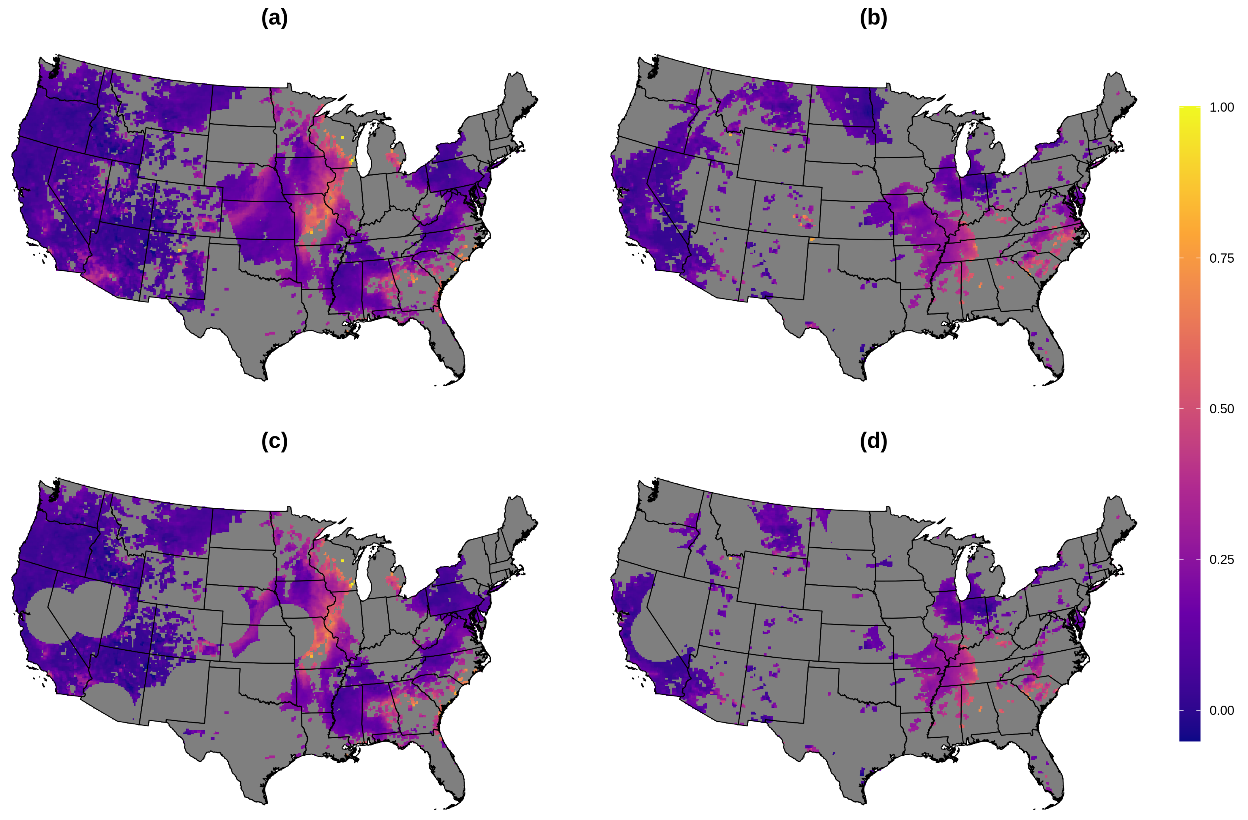
2.9. AOD Gap-Filling Analysis

From the observed AOD data, we consider a spatially clustered approach for creating a testing dataset on which to evaluate the results. In the proposed method, ten random AOD observations are selected from the observed AOD values for each day in July 2011. These observations and any other observations within a 250 km radius are then held out as the test dataset. We selected ten random points, in particular, to ensure that different areas of the observed data had a sufficient chance of being held out for the testing data, so that the performance of the different methods for a particular day was not likely to be judged solely on predictions for one area of the observed map. We also observed that this procedure resulted in close to a 70/30 split between training and testing data, on average. Figure 1 demonstrates the observed and training data on two particular days. This approach to creating testing data is an attempt to mimic the actual observed pattern of AOD data, where large contiguous areas are missing and require imputation. In particular, for many missing observations, there are likely no points nearby to aid in prediction. In our analysis, we consider each day separately for model fitting and prediction.

For RF and LK, we used validation data taken from the training data following a similar approach. For RF, we use 2000 trees with a node size of 5 and $m=7$. We include 22 variables: the projected centroid coordinates, elevation, the 2011 emission inventory, forest cover, impervious surface, total lengths of highway, limited-access road, and local road, population density, potential evaporation, surface DW longwave radiation flux, surface DW shortwave radiation flux, convective available potential energy, fraction of total precipitation that is convective, precipitation, relative humidity, temperature, u- and v-direction wind speed, pressure at surface, and GEOS-Chem AOD. For LK, we set the number of levels of resolution to 5, $a=12$, $\nu =0.1$, and the number of grid points along the largest dimension at the coarsest level of resolution to 15. By default, the LatticeKrig package includes the spatial coordinates as fixed predictors in $\mathit{Z}$. In addition, we include the interaction between the coordinates, GEOS-Chem, the interaction between each coordinate and GEOS-Chem, and elevation as the fixed predictors in the model. No variable selection was performed—we instead focused on tuning the spatial aspect of the model.

In addition to comparing RF and LK, we aim to consider SL approaches for combining these distinct methods. For each day, we construct 10 cross-validation folds using the blockCV R package (version 2.1.1) [49]. This constructs spatial blocks for the validation dataset, so that performance more accurately mimics the task of gap-filling AOD. In the Supplementary Materials (Figure S6), we provide a full set of the maps showing these spatial block cross-validation folds. Sarafian et al. [50], Murray et al. [35] (for PM_2.5 prediction) and Young et al. [51] (for NO₂) also consider spatially clustered cross-validation approaches for assessing model performance. Based on the cross-validation folds, we stack LK and RF validation predictions as discussed in the previous section. We assess 4 different methods for combining LK and RF:

• Average. We construct a simple average of RF and LK predictions. Cross-validation data are not used in this approach.
• SL: overall. After stacking all of the cross-validation predictions for all days together, we produce a single set of optimal weights with (4) for making predictions.
• SL: daily. We stack cross-validation predictions for each day separately, and we obtaining a daily set of optimal weights with (4).
• SL: distance-based. For each cross-validation fold on each day, we determine the closest distance between each point in the cross-validation fold and the training data. We then stack all of the cross-validation predictions across days together with these nearest-neighbor distances. We bin these stacked predictions according to nearest-neighbor distances with bin widths of 25 km from 0 to 300 km and higher. Using (4), we estimate the optimal weights for LK and RF for each binned distance grouping. We then fit a simple loess model relating interval mid-point distance and optimal weight, and we use these fitted optimal weights for combining LK and RF for predictions. The motivation for this last technique is that the further the unobserved point is from the observed data, the more different algorithms may be in predictions. If there is strong spatial correlation, then LK may perform better; in contrast, if there is limited range in the spatial correlation and the covariates are more important, then RF may produce better fits based on the relationship between the covariates and response.

In all cases, we restrict weights to be between 0.1 and 0.9. We primarily assess model performance on the basis of root mean square error (RMSE) and the coefficient of determination (R²), as well as the intercept and slope from a linear model relating the true AOD observations to the predicted values.

2.10. PM_2.5 Analysis

We compare several random forest models for PM_2.5 concentration estimation to determine whether including gap-filled AOD as a predictor can improve prediction performance. Our gap-filled AOD is based on the super learner distance-based method. There are five variations on the random forest models’ features:

• M1: Includes neither AOD nor GEOS-Chem.
• M2: Includes GEOS-Chem.
• M3: Includes gap-filled AOD. This variable is defined to be observed AOD where available, and otherwise the predicted AOD value based on the super-learner distance-based method. GEOS-Chem is also included as a separate feature.
• M4: Includes AOD by replacing missing values of AOD with GEOS-Chem (as in Hu et al. [17]).
• M5: Includes observed AOD, and training solely on observations where AOD is observed. For predictions, missing values of AOD are replaced with the gap-filled AOD. GEOS-Chem is also included as a separate feature.

The other features included in the random forest models are the same as those in the AOD analysis. All models except M5 additionally include an indicator variable for whether AOD was observed at the location, and all models include a so-called convolution layer of PM_2.5. Several analyses [17,34] have demonstrated that a weighted-average of nearby PM_2.5 observations can aid in model prediction for PM_2.5. Briefly, for each location, the convolution layer of PM_2.5 is a weighted average of all other training PM_2.5 observations, not including the location itself. The weights are inversely proportional to the squared distance between locations (less distant observations in the training data are weighted more). The procedure for creating the convolution PM_2.5 layer must be repeated for each training/validation split for each day.

We consider three distinct 10-fold cross-validation approaches for assessing performance:

• Random: Cross-validation folds are constructed by selecting observed PM_2.5 monitors at random on a daily basis.
• Constant spatial clusters: Cross-validation folds are constructed by creating spatially clustered areas that are constant across all days. A particular area of the map will be assigned to the same cross-validation fold for each day.
• Varying spatial clusters: Cross-validation folds are constructed by creating spatial clusters at random for each day.

Spatial clusters are constructed using the blockCV package (version 2.1.1) in R with block widths of 150 km. Figure S8 in the Supplemental Materials displays the constant spatial construction by color-coding monitor locations.

Models were fit both for each day separately, as well as for all of the days in July 2011 together. In the latter spatio-temporal random forest model, day of the year and day of the week are additionally included as integer predictor variables. Our primary metrics of interest are RMSE, R², and the full prediction maps, but we also present the intercept/slope estimates from fitting a linear regression model with the true PM_2.5 values as the dependent variable and the random forest prediction as the independent variable. For all models, we set the number of trees to 2000. We varied m (mtry) between values of 4, 8, 12, and 16 and presented the best results for each model and cross-validation fold type on the basis of RMSE. The full maps and feature importance results are based on $m=4$. The Supplemental Materials include additional figures and tables for $m=8$.

3. Results

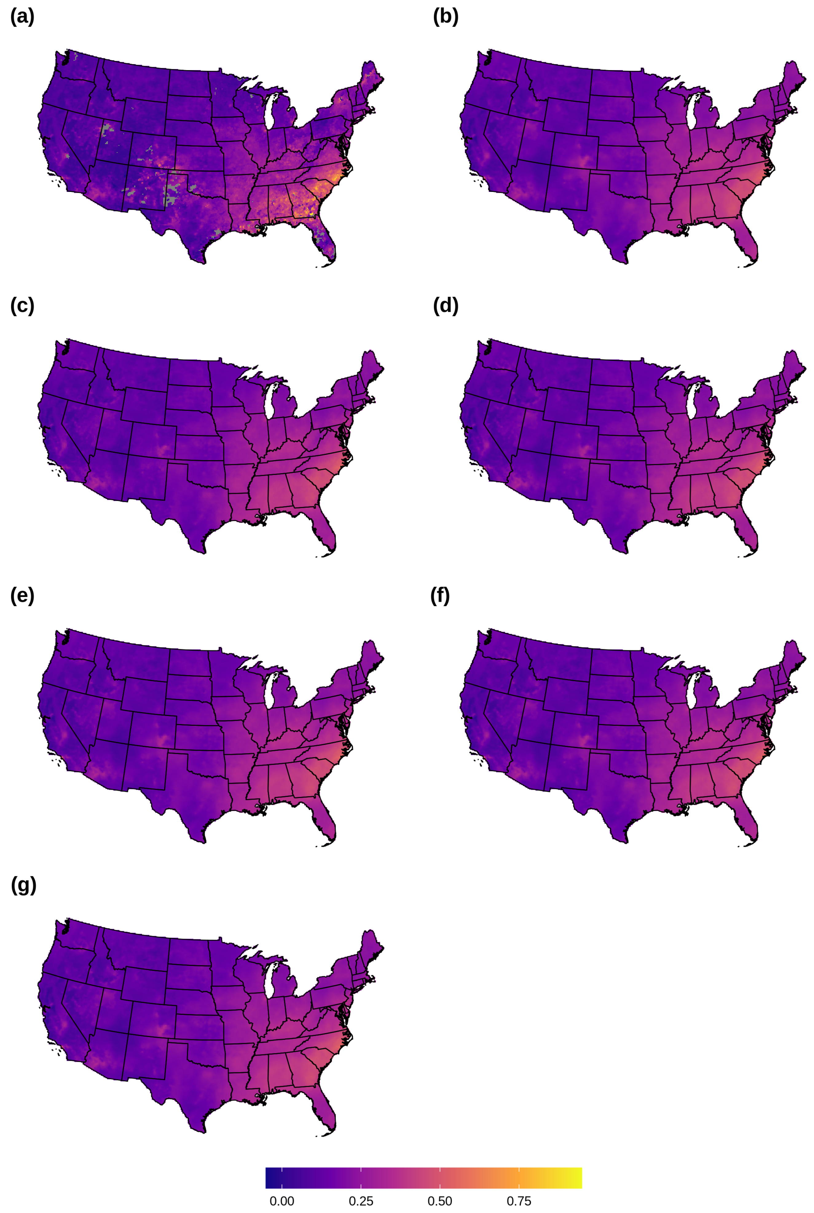
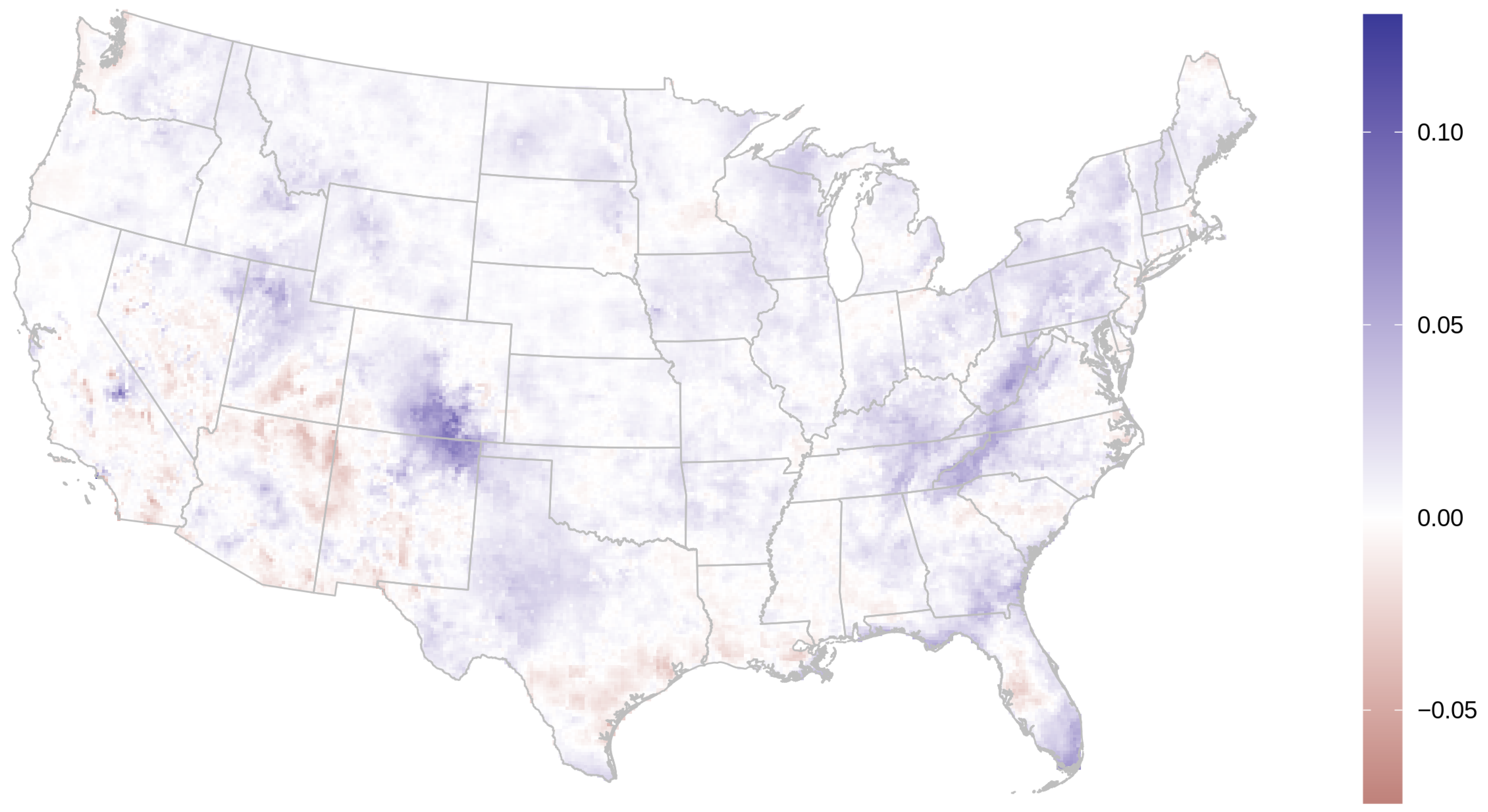
3.1. AOD Gap-Filling

We highlight several results from our analysis. First, daily results show that any of the average/super learner approaches match or exceed performance from either LK or RF alone on a majority of days on the basis of RMSE (

Table 1. Summary statistics on the combined test AOD predictions across all days of July 2011. The two right columns denote the number of days in which the method performed best or worst on the basis of root-mean-square error (RMSE).

Method					# of Days Ranked
	R2	RMSE (×100)	Intercept	Slope	Best	Worst
LatticeKrig	0.644	6.66	−0.01	0.94	7	12
Random Forest	0.619	6.90	−0.01	0.92	3	19
LK-RF Average	0.658	6.52	−0.01	0.97	4	0
SL: Overall	0.659	6.51	−0.01	0.97	4	0
SL: Daily	0.657	6.52	−0.01	0.96	3	0
SL: Distance-based	0.659	6.50	−0.01	0.96	10	0

, Figure S2). While there are some days where either LK or RF does particularly well, there are also days where these two methods perform worse than any of the other methods. The ensemble methods are the best or close to the best in terms of RMSE and R² on the majority of days. The distance-based SL method performs best on more days (10 out of 31 days) than any of the other approaches considered. Based on our described approach, the distance-based SL prediction weights LK greater for testing points that are close to training data, while for points further away from the training data, it weights RF more, relying on a combination of location, land use, and meteorological features (see Figure S7 in the Supplemental Materials).

Evaluating test predictions across all 31 days together, LK and RF have R² values of 0.644 and 0.619, respectively. The average and SL methods improve to R² values in the range of 0.657 to 0.659. Compared to LK alone, the RMSE is reduced 2.34% and 2.30% in the distance-based and overall SL models, respectively. A simple average of the LK and RF predictions also provides most of these gains. The super learner method based on the daily construction of weights performs well but is marginally worse than the other ensemble methods. In explaining this small difference in performance, we posit that the daily weight estimates may be slightly over-fitted to the daily training data relative to the other ensemble methods, which benefit from pooling cross-validation predictions across days together for the estimation of the super learner weights.

Both LK and RF methods diverge substantially from using just the observed AOD data in the July 2011 averages (Figure 2). LK and RF predictions are notably different from each other in the Appalachian Mountains and in parts of the Southwest, where LK predicts higher values relative to RF (Figure 3). There are also apparent edge effects in some areas such as south Florida, where LK predictions will tend to diverge more substantially from those of RF. These may be partly due to issues with LK’s coefficient estimation in areas where there are few data for a particular day (see Figures S3 and S4 in the Supplemental Materials for plots of daily AOD predictions and daily differences between LK and RF).

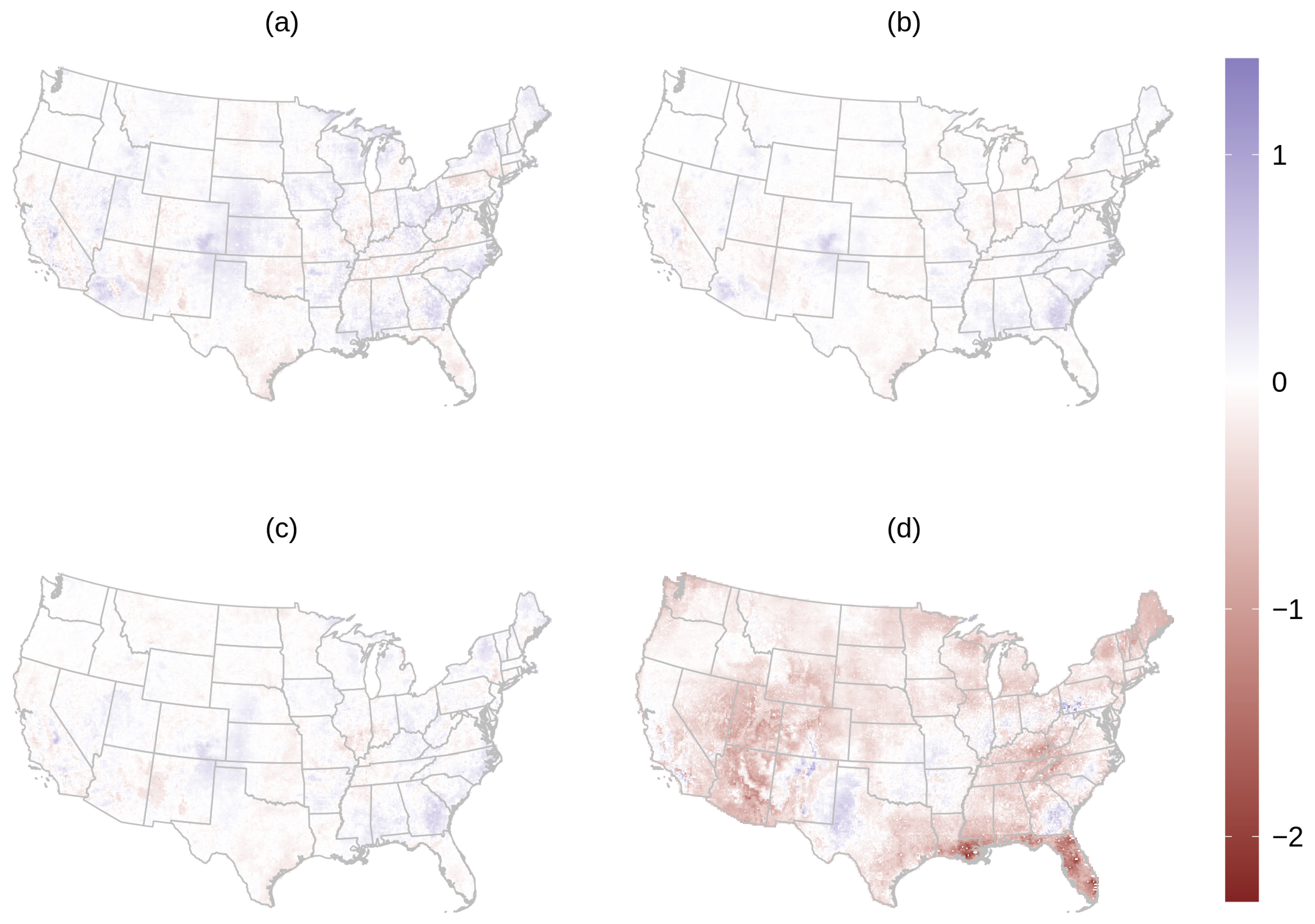
3.2. PM_2.5 Prediction

The gap-filled AOD used in the PM_2.5 analyses is based on the SL distance-based method for combining RF and LK predictions on the basis of the results in the AOD analysis. We first highlight a few notable results from the daily random forest models. First, the daily random forest models suggest that RMSE is improved consistently but only marginally by including the imputed AOD predictor vs. the four alternatives (

Table 2. R² and root mean square error (RMSE) result from the daily and spatio-temporal random forest models for three different 10-fold cross-validation settings. Summary metrics are evaluated on all observations as well as separately on the basis of AOD’s missingness status (observed or missing). The M3a and M3b random forest models include gap-filled AOD as a predictor.

		Daily					Spatio-Temporal
Setting	AOD Status	M1a	M2a	M3a	M4a	M5a	M1b	M2b	M3b	M4b	M5b
RMSE (μg m−3)
Random	All	3.30	3.29	3.28	3.30	3.68	2.96	2.98	2.99	2.98	3.20
Random	Missing	3.30	3.28	3.27	3.29	3.84	2.99	3.00	3.02	3.01	3.29
Random	Observed	3.31	3.30	3.29	3.31	3.41	2.92	2.94	2.95	2.94	3.04
Constant cluster	All	3.66	3.64	3.62	3.64	3.99	3.68	3.66	3.63	3.66	3.75
Constant cluster	Missing	3.61	3.58	3.56	3.59	4.09	3.63	3.60	3.57	3.61	3.74
Constant cluster	Observed	3.74	3.73	3.72	3.73	3.82	3.76	3.75	3.72	3.73	3.76
Varying cluster	All	3.66	3.65	3.63	3.65	4.00	3.33	3.34	3.35	3.35	3.56
Varying cluster	Missing	3.61	3.58	3.57	3.60	4.11	3.34	3.33	3.34	3.34	3.61
Varying cluster	Observed	3.75	3.74	3.72	3.74	3.83	3.33	3.35	3.35	3.35	3.47
R2 (×100)
Random	All	75.3	75.5	75.7	75.4	69.7	80.4	80.2	79.8	80.0	77.1
Random	Missing	75.9	76.2	76.3	76.1	68.1	80.5	80.4	79.9	80.1	76.5
Random	Observed	73.8	73.9	74.1	73.8	72.3	79.9	79.7	79.3	79.5	78.0
Constant cluster	All	69.9	70.1	70.4	70.1	64.1	69.6	69.9	70.3	69.9	68.6
Constant cluster	Missing	71.5	71.8	72.2	71.7	63.6	71.2	71.6	72.1	71.5	69.8
Constant cluster	Observed	66.8	66.9	67.2	66.9	65.2	66.4	66.7	67.1	66.8	66.6
Varying cluster	All	69.7	70.0	70.3	70.0	63.9	75.6	75.6	75.4	75.5	72.1
Varying cluster	Missing	71.4	71.8	72.1	71.7	63.2	76.3	76.4	76.2	76.3	72.2
Varying cluster	Observed	66.5	66.6	67.1	66.7	65.1	74.1	73.9	73.9	73.7	71.8

, M3a). The outlier model is M5, which trains solely on observations where AOD is observed and predicts using the imputed AOD where AOD is missing. The results from model M5 are substantially worse than the other models, with a relatively biased prediction map (Figure 4d). For the remainder of the results, we omit discussion of this model. Generally, the gain in RMSE for the model using gap-filled AOD (M3) is small and ranges from 0.01 to 0.03 μg m⁻³ against the other models. The results for R² are similar, with small gains of approximately 0.002 to 0.006. Second, the daily random forest models tended to have better PM_2.5 prediction in locations where AOD was not observed as compared to areas where AOD was observed, regardless of the features included. Third, cross-validated RMSE is substantially larger in spatial cross-validation settings than in the case with folds consisting of randomly selected locations.

The spatio-temporal random forest results in the second set of columns in Table 2 show somewhat different patterns. RMSE and R² are generally improved over the daily models for the random and varying spatially clustered cross-validation analyses, but there is no longer a benefit to including imputed AOD. On the contrary, the model predictions tend to do better when neither AOD nor GEOS-Chem are included on the basis of R² and RMSE. The exception to these results are in the constant spatially clustered cross-validation setting—here, there is some very marginal improvement from including imputed AOD over the other models. We posit that in spatio-temporal models, multiple days’ observations in the same area as where we intend to make a prediction on a different day can largely diminish the predictive power of AOD. However, when the same spatial area is consistently missing, the model can no longer rely on other days’ observations for the same area to improve prediction accuracy. Notably, this setting mirrors qualities of producing full maps of PM_2.5 observations. Given that there is a fixed network of monitors (not all of which operate on every day), PM_2.5 prediction is primarily focused on areas where there is never a monitor present. We emphasize that the percentage decrease in RMSE from including the imputed AOD in this constant spatially clustered cross-validation setting for the spatio-temporal random forest models is small at 1.25%, 0.67%, and 0.77% compared to the models with no AOD or GEOS-Chem, just GEOS-Chem, or the combined AOD/GEOS-Chem variable, respectively. Notably in this case, daily models slightly outperform the performance of the spatio-temporal models. In the other cross-validation settings, RMSE and R² both improve substantially from fitting a full spatio-temporal model over a series of daily models.

Results for RMSE and R² by region (as defined by NOAA) and cross-validation setting are also provided in

Table 3. Regional root-mean-square error (RMSE) results (μg m⁻³) for daily and spatio-temporal random forest model for different 10-fold cross-validation settings. The M3a and M3b random forest models include gap-filled AOD as a predictor.

		Daily					Spatio-Temporal
Setting	AOD Status	M1a	M2a	M3a	M4a	M5a	M1b	M2b	M3b	M4b	M5b
Random	Central	3.70	3.67	3.65	3.68	4.15	3.56	3.56	3.58	3.56	3.78
	East North Central	3.17	3.17	3.16	3.18	3.52	3.04	3.03	3.01	3.02	3.15
	Northeast	3.31	3.27	3.26	3.29	3.74	2.97	2.96	3.00	2.97	3.23
	Northwest	1.48	1.49	1.49	1.49	1.82	1.23	1.24	1.24	1.24	1.35
	South	2.35	2.35	2.33	2.35	2.77	2.11	2.13	2.15	2.15	2.39
	Southeast	3.55	3.54	3.53	3.56	4.22	3.39	3.41	3.40	3.43	3.72
	Southwest	4.13	4.11	4.09	4.10	4.43	3.58	3.61	3.62	3.54	3.94
	West	4.41	4.42	4.41	4.40	4.47	3.58	3.64	3.70	3.67	3.76
	West North Central	2.91	2.92	2.92	2.92	3.08	2.34	2.37	2.35	2.35	2.50
Constant cluster	Central	4.38	4.34	4.32	4.34	4.67	4.54	4.49	4.46	4.50	4.60
	East North Central	3.36	3.36	3.34	3.36	3.67	3.46	3.41	3.38	3.43	3.48
	Northeast	3.55	3.51	3.49	3.53	3.90	3.54	3.49	3.46	3.50	3.60
	Northwest	1.48	1.48	1.50	1.49	1.84	1.46	1.46	1.46	1.46	1.53
	South	2.47	2.47	2.46	2.47	2.90	2.49	2.47	2.47	2.48	2.64
	Southeast	3.91	3.88	3.83	3.90	4.54	3.94	3.92	3.85	3.93	4.08
	Southwest	4.29	4.27	4.26	4.27	4.60	4.34	4.34	4.35	4.32	4.47
	West	5.20	5.21	5.21	5.19	5.28	5.10	5.11	5.08	5.08	5.08
	West North Central	3.04	3.04	3.04	3.04	3.18	3.09	3.08	3.08	3.08	3.09
Varying cluster	Central	4.39	4.34	4.32	4.34	4.70	4.29	4.26	4.26	4.27	4.50
	East North Central	3.34	3.35	3.34	3.34	3.74	3.30	3.29	3.28	3.29	3.37
	Northeast	3.53	3.49	3.49	3.51	3.94	3.26	3.23	3.27	3.25	3.49
	Northwest	1.51	1.51	1.52	1.53	1.85	1.29	1.30	1.31	1.31	1.39
	South	2.48	2.49	2.48	2.49	2.93	2.31	2.33	2.34	2.33	2.59
	Southeast	3.92	3.89	3.84	3.92	4.54	3.76	3.74	3.70	3.75	4.03
	Southwest	4.45	4.44	4.42	4.42	4.76	3.97	4.02	4.07	4.02	4.30
	West	5.16	5.17	5.14	5.16	5.18	4.18	4.23	4.26	4.25	4.42
	West North Central	2.97	2.97	2.97	2.97	3.11	2.40	2.43	2.45	2.45	2.57

and

Table 4. Regional R² (×100) results for daily and spatio-temporal random forest model for different 10-fold cross-validation settings. The M3a and M3b random forest models include gap-filled AOD as a predictor.

		Daily					Spatio-Temporal
Setting	AOD Status	M1a	M2a	M3a	M4a	M5a	M1b	M2b	M3b	M4b	M5b
Random	Central	61.1	61.7	62.1	61.5	51.1	64.7	64.7	63.8	64.1	59.3
	East North Central	69.4	69.6	69.7	69.3	63.3	72.8	73.2	72.6	72.5	70.7
	Northeast	77.0	77.6	77.8	77.4	70.8	81.9	82.0	81.3	81.6	78.4
	Northwest	44.6	44.2	44.0	44.5	28.2	61.2	60.9	60.0	60.1	53.6
	South	68.0	68.1	68.4	68.0	57.9	74.5	74.0	73.2	73.1	67.5
	Southeast	70.4	70.6	70.8	70.2	59.5	73.2	73.1	72.8	72.3	68.3
	Southwest	46.6	47.3	47.7	47.4	42.4	61.1	60.6	59.3	61.0	51.9
	West	50.7	50.5	50.8	50.9	49.2	68.7	67.7	65.7	66.4	64.8
	West North Central	39.2	39.1	38.9	38.8	33.3	61.5	60.4	60.6	60.7	55.3
Constant cluster	Central	48.0	49.0	49.4	49.2	40.1	45.0	46.0	46.7	45.9	43.5
	East North Central	66.0	66.1	66.6	66.2	60.8	64.4	65.6	66.3	65.1	65.1
	Northeast	73.8	74.4	74.7	74.1	68.1	74.0	74.7	75.1	74.5	73.3
	Northwest	45.4	45.0	44.3	45.0	29.1	45.6	45.6	45.3	45.5	43.7
	South	64.5	64.6	64.9	64.5	53.5	64.3	64.9	65.0	64.6	61.5
	Southeast	64.4	64.9	65.9	64.5	53.5	64.1	64.4	65.6	64.2	62.5
	Southwest	41.9	42.5	42.8	42.6	35.1	40.5	40.4	40.3	40.9	37.5
	West	34.6	34.6	34.5	35.1	32.0	36.6	36.6	37.3	37.2	37.5
	West North Central	34.0	34.1	34.1	34.0	28.8	32.1	32.4	32.6	32.4	31.6
Varying cluster	Central	47.3	48.5	48.9	48.6	39.0	50.8	51.4	51.5	51.5	45.4
	East North Central	66.5	66.5	66.7	66.5	59.1	68.5	69.1	69.3	69.0	67.4
	Northeast	74.3	74.8	74.9	74.6	67.6	79.0	79.3	78.7	79.1	75.3
	Northwest	42.5	42.4	42.0	41.9	26.7	58.1	57.7	57.0	56.8	52.1
	South	64.3	64.2	64.4	64.1	52.7	70.2	69.9	69.6	69.8	63.1
	Southeast	64.3	64.8	65.8	64.2	53.2	68.0	68.3	69.0	68.1	63.5
	Southwest	37.5	37.8	38.5	38.5	30.6	53.0	52.0	50.9	52.8	43.7
	West	33.8	33.6	34.4	34.1	32.8	58.8	57.7	57.3	57.5	52.4
	West North Central	36.6	36.7	36.8	36.6	31.4	59.8	58.8	58.1	58.4	53.4

. RMSE results tend to be worst in the West, Southwest, and Central regions across cross-validation settings. Notably, although RMSE is quite low for the Northwest region, the R² for this area is comparatively low, suggesting low pollution levels but also poor prediction performance from the models. The spatio-temporal models improve the regional RMSE and R² as compared to the daily models, except for the constant spatially clustered cross-validation setting, where there is variability in changes in regional performance. Variable importance metrics for the $m=4$ setting based on the spatio-temporal models are presented in Table S1 using the permutation-based method [23]. Briefly, this importance metric denotes the increase in mean-squared error on the OOB sample for each tree after permuting the values of the feature. On this basis, the convolution layer of PM_2.5 is the most important predictor for these models. When imputed AOD is included, the relative importance of several other variables is slightly diminished. While imputed AOD is not the most important feature, it appears substantively important on the basis of a mean decrease in accuracy. Additional feature importance tables are provided in the Supplemental Materials for $m=8$ (Table S2). In general, for larger m, the convolution layer of PM_2.5 becomes more important—it is more likely to be selected as the optimal feature for splitting a node as m increases, and it is a particularly strong predictor.

When comparing model M3 to models M1, M2, and M4, the average of monthly mean differences are close to 0 μg m⁻³, but the monthly mean differences are apparently spatially correlated (Figure 4). The model trained only on points where AOD is observed (M5) leads to over-estimated average monthly values of PM_2.5 relative to the model using gap-filled AOD, with an average difference of 0.25 μg m⁻³. The standard deviation of daily differences for all grid cells for July 2011 is 0.44 μg m⁻³ for M3 and M1, 0.32 μg m⁻³ for M3 and M2, and 0.38 μg m⁻³ for M3 and M4, suggesting small but meaningful variability in the daily model predictions. Some of the largest daily differences between models tend to be in areas with sparse air pollution monitors (Figure S11). Figure 5 shows the July 2011 averaged values from M3 with the gap-filled AOD as a feature in the spatio-temporal random forest model.

2

4. Discussion

We highlight the main findings of this study in three points. First, we emphasize the importance of constructing testing and cross-validation data that mimic the missing data patterns for both AOD and PM_2.5 prediction. Previously reported metrics for AOD gap-filling using RF may be over-stated if using out-of-bag (OOB) metrics [10,24], as using large contiguous areas for testing suggests substantially lower R². Different cross-validation settings for PM_2.5 model evaluation also suggest that performance varies considerably based on the manner of holdout, echoing the findings of previous studies that “spatial” cross-validation performance metrics are typically worse than random cross-validation metrics. In our study, our spatial cross-validation procedures leave out spatially clustered sets of monitors as in several recent studies [35,50,51]. Our results show roughly similar performance metrics for PM_2.5 estimation compared to previous RF results when using the random cross-validation setting, with ≈0.80 (≈2.99) vs. 0.81 (2.78) R² (RMSE) for summer 2011 in Hu et al. [17]. The small difference in performance in our model as compared to that of Hu et al. [17] is likely because we fit the model solely to data in July 2011 rather than the full year, and because we did not include additional variables such as convolutional layers for land use terms, which have been shown to improve overall performance.

Second, we demonstrate how super learner approaches combining a large-scale spatial statistical method and machine learning predictions can improve upon the performance of each constituent predictor, and how the super learner method can be further modified for the particular task of AOD gap-filling. Future work should examine extensions to more machine learning and spatial statistical methods. For example, several recent studies have highlighted a number of spatial statistical methods with promising predictive performance and low computational costs [30,31,52,53,54,55,56,57,58], and using these in an ensemble approach may provide further improvements. Spatial data present additional theoretical challenges for super learner methods, given that the training data and testing data will generally not be independent of each other [48]. A limitation of the current study is the limited time frame and the use of daily rather than spatio-temporal AOD gap-filling models. We focused on July 2011 as there was, on average, less missingness in AOD in the summer than in other months, and we limited our analysis to a single month due to the high computational cost of fitting daily models with 10-fold cross-validation for the super learner. Future studies may consider expanding the time frame of spatial prediction beyond a month and including spatio-temporal statistical models that may better utilize the available observed data.

Finally, we demonstrate that imputed AOD using our proposed ensemble method can have a very small impact on particular RF models for estimating PM_2.5 concentrations, depending on the cross-validation setting. With a convolution layer of PM_2.5 and a rich set of other features, we generally find that AOD (imputed or not) is not strictly needed for good prediction of PM_2.5 in RF models as judged by R² and RMSE. However, population-level metrics like R² and RMSE may be misleading in masking improved small-scale predictions, and we find subtle differences in the predicted values between models, with and without gap-filled AOD as a predictor. Similarly, Huang et al. [25] find meaningful differences in daily PM_2.5 predictions in models with and without AOD as a predictor, particularly in areas of the map with sparse PM_2.5 monitors and on high-pollution days. Thus, although gap-filling AOD in the proposed ensemble approach adds to the computational costs of making PM_2.5 predictions, as compared to fitting a model without AOD as a predictor, there may be some marginal benefit to the quality of PM_2.5 predictions. A limitation of the current study is the lack of certain variables for AOD gap-filling and PM_2.5 estimation; previous work has found that the inclusion of cloud and snow fractions may improve AOD gap-filling and produce meaningful visual improvements in PM_2.5 estimation [10]. Moreover, finer resolution AOD products such as multi-angle implementation of atmospheric correction (MAIAC)-derived AOD may provide greater predictive power for PM_2.5 [59] at the expense of increasing the computational costs of gap-filling. Future studies should examine the computational costs and benefits of using the proposed method to gap-fill AOD for predicting PM_2.5 at the 1 km resolution.

5. Conclusions

This article considered a recently developed large-scale spatial statistical method (LK), a popular machine learning method (RF), and various combinations of these methods for gap-filling daily MODIS AOD on a 12 km × 12 km grid in the contiguous United States in July 2011. Using large contiguous areas as holdouts for our performance comparison, we found that ensemble approaches can improve daily AOD gap-filling as compared to the individual methods on their own, on the basis of RMSE and R². The ultimate goal of making improvements in gap-filling AOD is to improve the performance of PM_2.5 prediction models and to provide complete spatial coverage. For this task, we compared several daily and spatio-temporal random forest models, with and without the inclusion of gap-filled AOD as a predictor. These results were mixed, showing very small but consistent improvements to RMSE and R² by including the gap-filled AOD in the daily models, but varying results in the spatio-temporal models. However, in the more realistic spatially clustered cross-validation setting, where spatial clusters of the observed locations are assigned to the same cross-validation fold for all days, we find small improvements for PM_2.5 from including the gap-filled AOD predictor. Furthermore, although the differences in RMSE and R² are small, daily prediction maps suggest some meaningful differences between the considered models, particularly in areas with sparse monitoring locations. Future research should extend this work by considering computationally efficient spatio-temporal statistical approaches for gap-filling AOD (as compared to daily gap-filling models), increasing the time frame of study, and considering gap-filling at finer resolutions (e.g., MAIAC AOD at 1 km resolution).

References

1. WHO. Ambient (Outdoor) Air Pollution. 2018. Available online: https://web.archive.org/web/20200824220508/https%3A%2F%2Fwww.who.int%2Fnews-room%2Ffact-sheets%2Fdetail%2Fambient-%2528outdoor%2529-air-quality-and-health (accessed on 24 August 2020).
2. Lim, S.S.; Vos, T.; Flaxman, A.D.; Danaei, G.; Shibuya, K.; Adair-Rohani, H.; AlMazroa, M.A.; Amann, M.; Anderson, H.R.; Andrews, K.G.; et al. A comparative risk assessment of burden of disease and injury attributable to 67 risk factors and risk factor clusters in 21 regions, 1990–2010: A systematic analysis for the Global Burden of Disease Study 2010. Lancet 2012, 380, 2224–2260. [Google Scholar] [CrossRef] [Green Version]
3. Lelieveld, J.; Evans, J.S.; Fnais, M.; Giannadaki, D.; Pozzer, A. The contribution of outdoor air pollution sources to premature mortality on a global scale. Nature 2015, 525, 367–371. [Google Scholar] [CrossRef] [PubMed]
4. Levy, R.; Mattoo, S.; Munchak, L.; Remer, L.; Sayer, A.; Patadia, F.; Hsu, N. The Collection 6 MODIS aerosol products over land and ocean. Atmos. Meas. Tech. 2013, 6, 2989. [Google Scholar] [CrossRef] [Green Version]
5. Sorek-Hamer, M.; Just, A.; Kloog, I. Satellite remote sensing in epidemiological studies. Curr. Opin. Pediatr. 2016, 28, 228. [Google Scholar] [CrossRef] [PubMed] [Green Version]
6. Chu, Y.; Liu, Y.; Li, X.; Liu, Z.; Lu, H.; Lu, Y.; Mao, Z.; Chen, X.; Li, N.; Ren, M.; et al. A review on predicting ground PM2.5 concentration using satellite aerosol optical depth. Atmosphere 2016, 7, 129. [Google Scholar] [CrossRef] [Green Version]
7. Shin, M.; Kang, Y.; Park, S.; Im, J.; Yoo, C.; Quackenbush, L.J. Estimating ground-level particulate matter concentrations using satellite-based data: A review. GIScience Remote Sens. 2020, 57, 174–189. [Google Scholar] [CrossRef]
8. Belle, J.H.; Liu, Y. Evaluation of Aqua MODIS Collection 6 AOD Parameters for Air Quality Research over the Continental United States. Remote Sens. 2016, 8, 815. [Google Scholar] [CrossRef] [Green Version]
9. Belle, J.H.; Chang, H.H.; Wang, Y.; Hu, X.; Lyapustin, A.; Liu, Y. The potential impact of satellite-retrieved cloud parameters on ground-level PM2.5 mass and composition. Int. J. Environ. Res. Public Health 2017, 14, 1244. [Google Scholar] [CrossRef] [Green Version]
10. Bi, J.; Belle, J.H.; Wang, Y.; Lyapustin, A.I.; Wildani, A.; Liu, Y. Impacts of snow and cloud covers on satellite-derived PM2.5 levels. Remote Sens. Environ. 2019, 221, 665–674. [Google Scholar] [CrossRef]
11. Christopher, S.A.; Gupta, P. Satellite remote sensing of particulate matter air quality: The cloud-cover problem. J. Air Waste Manag. Assoc. 2010, 60, 596–602. [Google Scholar] [CrossRef]
12. Liang, F.; Xiao, Q.; Huang, K.; Yang, X.; Liu, F.; Li, J.; Lu, X.; Liu, Y.; Gu, D. The 17-y spatiotemporal trend of PM2.5 and its mortality burden in China. Proc. Natl. Acad. Sci. USA 2020, 117, 25601–25608. [Google Scholar] [CrossRef] [PubMed]
13. Geng, G.; Murray, N.L.; Tong, D.; Fu, J.S.; Hu, X.; Lee, P.; Meng, X.; Chang, H.H.; Liu, Y. Satellite-Based Daily PM2.5 Estimates During Fire Seasons in Colorado. J. Geophys. Res. Atmos. 2018, 123, 8159–8171. [Google Scholar] [CrossRef] [PubMed]
14. Kloog, I.; Koutrakis, P.; Coull, B.A.; Lee, H.J.; Schwartz, J. Assessing temporally and spatially resolved PM2.5 exposures for epidemiological studies using satellite aerosol optical depth measurements. Atmos. Environ. 2011, 45, 6267–6275. [Google Scholar] [CrossRef]
15. Kloog, I.; Nordio, F.; Coull, B.A.; Schwartz, J. Incorporating local land use regression and satellite aerosol optical depth in a hybrid model of spatiotemporal PM2.5 exposures in the Mid-Atlantic states. Environ. Sci. Technol. 2012, 46, 11913–11921. [Google Scholar] [CrossRef] [PubMed] [Green Version]
16. Lee, M.; Kloog, I.; Chudnovsky, A.; Lyapustin, A.; Wang, Y.; Melly, S.; Coull, B.; Koutrakis, P.; Schwartz, J. Spatiotemporal prediction of fine particulate matter using high-resolution satellite images in the Southeastern US 2003–2011. J. Expo. Sci. Environ. Epidemiol. 2016, 26, 377–384. [Google Scholar] [CrossRef] [PubMed] [Green Version]
17. Hu, X.; Belle, J.H.; Meng, X.; Wildani, A.; Waller, L.A.; Strickland, M.J.; Liu, Y. Estimating PM2.5 concentrations in the conterminous United States using the random forest approach. Environ. Sci. Technol. 2017, 51, 6936–6944. [Google Scholar] [CrossRef]
18. Xiao, Q.; Wang, Y.; Chang, H.H.; Meng, X.; Geng, G.; Lyapustin, A.; Liu, Y. Full-coverage high-resolution daily PM2.5 estimation using MAIAC AOD in the Yangtze River Delta of China. Remote Sens. Environ. 2017, 199, 437–446. [Google Scholar] [CrossRef]
19. Huang, K.; Xiao, Q.; Meng, X.; Geng, G.; Wang, Y.; Lyapustin, A.; Gu, D.; Liu, Y. Predicting monthly high-resolution PM2.5 concentrations with random forest model in the North China Plain. Environ. Pollut. 2018, 242, 675–683. [Google Scholar] [CrossRef]
20. Lv, B.; Hu, Y.; Chang, H.H.; Russell, A.G.; Bai, Y. Improving the accuracy of daily PM2.5 distributions derived from the fusion of ground-level measurements with aerosol optical depth observations, a case study in North China. Environ. Sci. Technol. 2016, 50, 4752–4759. [Google Scholar] [CrossRef]
21. Laslett, G.M. Kriging and splines: An empirical comparison of their predictive performance in some applications. J. Am. Stat. Assoc. 1994, 89, 391–400. [Google Scholar] [CrossRef]
22. Chen, Z.Y.; Zhang, T.H.; Zhang, R.; Zhu, Z.M.; Yang, J.; Chen, P.Y.; Ou, C.Q.; Guo, Y. Extreme gradient boosting model to estimate PM2.5 concentrations with missing-filled satellite data in China. Atmos. Environ. 2019, 202, 180–189. [Google Scholar] [CrossRef]
23. Breiman, L. Random forests. Mach. Learn. 2001, 45, 5–32. [Google Scholar] [CrossRef] [Green Version]
24. Stafoggia, M.; Bellander, T.; Bucci, S.; Davoli, M.; De Hoogh, K.; De’Donato, F.; Gariazzo, C.; Lyapustin, A.; Michelozzi, P.; Renzi, M.; et al. Estimation of daily PM10 and PM2.5 concentrations in Italy, 2013–2015, using a spatiotemporal land-use random-forest model. Environ. Int. 2019, 124, 170–179. [Google Scholar] [CrossRef]
25. Huang, K.; Bi, J.; Meng, X.; Geng, G.; Lyapustin, A.; Lane, K.J.; Gu, D.; Kinney, P.L.; Liu, Y. Estimating daily PM2.5 concentrations in New York City at the neighborhood-scale: Implications for integrating non-regulatory measurements. Sci. Total Environ. 2019, 697, 134094. [Google Scholar] [CrossRef] [PubMed]
26. Zhang, R.; Di, B.; Luo, Y.; Deng, X.; Grieneisen, M.L.; Wang, Z.; Yao, G.; Zhan, Y. A nonparametric approach to filling gaps in satellite-retrieved aerosol optical depth for estimating ambient PM2.5 levels. Environ. Pollut. 2018, 243, 998–1007. [Google Scholar] [CrossRef]
27. Jiang, T.; Chen, B.; Nie, Z.; Ren, Z.; Xu, B.; Tang, S. Estimation of hourly full-coverage PM2.5 concentrations at 1-km resolution in China using a two-stage random forest model. Atmos. Res. 2021, 248, 105146. [Google Scholar] [CrossRef]
28. Holben, B.N.; Eck, T.F.; Slutsker, I.A.; Tanre, D.; Buis, J.; Setzer, A.; Vermote, E.; Reagan, J.A.; Kaufman, Y.; Nakajima, T.; et al. AERONET—A federated instrument network and data archive for aerosol characterization. Remote Sens. Environ. 1998, 66, 1–16. [Google Scholar] [CrossRef]
29. Sayer, A.; Munchak, L.; Hsu, N.; Levy, R.; Bettenhausen, C.; Jeong, M.J. MODIS Collection 6 aerosol products: Comparison between Aqua’s e-Deep Blue, Dark Target, and “merged” data sets, and usage recommendations. J. Geophys. Res. Atmos. 2014, 119, 13–965. [Google Scholar] [CrossRef]
30. Heaton, M.J.; Datta, A.; Finley, A.O.; Furrer, R.; Guinness, J.; Guhaniyogi, R.; Gerber, F.; Gramacy, R.B.; Hammerling, D.; Katzfuss, M.; et al. A case study competition among methods for analyzing large spatial data. J. Agric. Biol. Environ. Stat. 2019, 24, 398–425. [Google Scholar] [CrossRef] [Green Version]
31. Bradley, J.R.; Cressie, N.; Shi, T. A comparison of spatial predictors when datasets could be very large. Stat. Surv. 2016, 10, 100–131. [Google Scholar] [CrossRef]
32. Shao, Y.; Ma, Z.; Wang, J.; Bi, J. Estimating daily ground-level PM2.5 in China with random-forest-based spatiotemporal kriging. Sci. Total Environ. 2020, 740, 139761. [Google Scholar] [CrossRef] [PubMed]
33. Xiao, Q.; Chang, H.H.; Geng, G.; Liu, Y. An ensemble machine-learning model to predict historical PM2.5 concentrations in China from satellite data. Environ. Sci. Technol. 2018, 52, 13260–13269. [Google Scholar] [CrossRef] [PubMed]
34. Di, Q.; Amini, H.; Shi, L.; Kloog, I.; Silvern, R.; Kelly, J.; Sabath, M.B.; Choirat, C.; Koutrakis, P.; Lyapustin, A.; et al. An ensemble-based model of PM2.5 concentration across the contiguous United States with high spatiotemporal resolution. Environ. Int. 2019, 130, 104909. [Google Scholar] [CrossRef] [PubMed]
35. Murray, N.L.; Holmes, H.A.; Liu, Y.; Chang, H.H. A Bayesian ensemble approach to combine PM2.5 estimates from statistical models using satellite imagery and numerical model simulation. Environ. Res. 2019, 178, 108601. [Google Scholar] [CrossRef] [PubMed]
36. Nychka, D.; Bandyopadhyay, S.; Hammerling, D.; Lindgren, F.; Sain, S. A multiresolution Gaussian process model for the analysis of large spatial datasets. J. Comput. Graph. Stat. 2015, 24, 579–599. [Google Scholar] [CrossRef] [Green Version]
37. van der Laan, M.J.; Polley, E.C.; Hubbard, A.E. Super learner. Stat. Appl. Genet. Mol. Biol. 2007, 6. [Google Scholar] [CrossRef]
38. Naimi, A.I.; Balzer, L.B. Stacked generalization: An introduction to super learning. Eur. J. Epidemiol. 2018, 33, 459–464. [Google Scholar] [CrossRef]
39. Levy, R.; Hsu, C. MODIS Atmosphere L2 Aerosol Product. NASA MODIS Adaptive Processing System; Goddard Space Flight Center: Greenbelt, MD, USA, 2015; Vulume 10. [CrossRef]
40. Bey, I.; Jacob, D.J.; Yantosca, R.M.; Logan, J.A.; Field, B.D.; Fiore, A.M.; Li, Q.; Liu, H.Y.; Mickley, L.J.; Schultz, M.G. Global modeling of tropospheric chemistry with assimilated meteorology: Model description and evaluation. J. Geophys. Res. Atmos. 2001, 106, 23073–23095. [Google Scholar] [CrossRef]
41. Li, S.; Garay, M.J.; Chen, L.; Rees, E.; Liu, Y. Comparison of GEOS-Chem aerosol optical depth with AERONET and MISR data over the contiguous United States. J. Geophys. Res. Atmos. 2013, 118, 11–228. [Google Scholar] [CrossRef]
42. Cosgrove, B.A.; Lohmann, D.; Mitchell, K.E.; Houser, P.R.; Wood, E.F.; Schaake, J.C.; Robock, A.; Marshall, C.; Sheffield, J.; Duan, Q.; et al. Real-time and retrospective forcing in the North American Land Data Assimilation System (NLDAS) project. J. Geophys. Res. Atmos. 2003, 108. [Google Scholar] [CrossRef] [Green Version]
43. Mitchell, K.E.; Lohmann, D.; Houser, P.R.; Wood, E.F.; Schaake, J.C.; Robock, A.; Cosgrove, B.A.; Sheffield, J.; Duan, Q.; Luo, L.; et al. The multi-institution North American Land Data Assimilation System (NLDAS): Utilizing multiple GCIP products and partners in a continental distributed hydrological modeling system. J. Geophys. Res. Atmos. 2004, 109. [Google Scholar] [CrossRef] [Green Version]
44. Nychka, D.; Hammerling, D.; Sain, S.; Lenssen, N. LatticeKrig: Multiresolution Kriging Based on Markov Random Fields. R Package Version 8.4, 2016. Available online: https://cran.r-project.org/web/packages/LatticeKrig/index.html (accessed on 30 December 2020). [CrossRef]
45. Wright, M.N.; Ziegler, A. ranger: A Fast Implementation of Random Forests for High Dimensional Data in C++ and R. J. Stat. Softw. 2017, 77. [Google Scholar] [CrossRef] [Green Version]
46. Breiman, L. Stacked regressions. Mach. Learn. 1996, 24, 49–64. [Google Scholar] [CrossRef] [Green Version]
47. Polley, E.C.; van der Laan, M.J. Super learner in prediction. In U.C. Berkeley Division of Biostatistics Working Paper Series. Working Paper 266; U.C. Berkeley: Berkeley, CA, USA, 2010. [Google Scholar]
48. Davies, M.M.; van der Laan, M.J. Optimal spatial prediction using ensemble machine learning. Int. J. Biostat. 2016, 12, 179–201. [Google Scholar] [CrossRef] [Green Version]
49. Valavi, R.; Elith, J.; Lahoz-Monfort, J.J.; Guillera-Arroita, G. blockCV: An R package for generating spatially or environmentally separated folds for k-fold cross-validation of species distribution models. Methods Ecol. Evol. 2019, 10, 225–232. [Google Scholar] [CrossRef] [Green Version]
50. Sarafian, R.; Kloog, I.; Just, A.C.; Rosenblatt, J.D. Gaussian Markov Random Fields versus Linear Mixed Models for satellite-based PM2.5 assessment: Evidence from the Northeastern USA. Atmos. Environ. 2019, 205, 30–35. [Google Scholar] [CrossRef] [Green Version]
51. Young, M.T.; Bechle, M.J.; Sampson, P.D.; Szpiro, A.A.; Marshall, J.D.; Sheppard, L.; Kaufman, J.D. Satellite-based NO2 and model validation in a national prediction model based on universal kriging and land-use regression. Environ. Sci. Technol. 2016, 50, 3686–3694. [Google Scholar] [CrossRef] [Green Version]
52. Cressie, N.; Shi, T.; Kang, E.L. Fixed rank filtering for spatio-temporal data. J. Comput. Graph. Stat. 2010, 19, 724–745. [Google Scholar] [CrossRef] [Green Version]
53. Lindgren, F.; Rue, H.; Lindström, J. An explicit link between Gaussian fields and Gaussian Markov random fields: The stochastic partial differential equation approach. J. R. Stat. Soc. Ser. B Stat. Methodol. 2011, 73, 423–498. [Google Scholar] [CrossRef] [Green Version]
54. Datta, A.; Banerjee, S.; Finley, A.O.; Gelfand, A.E. Hierarchical nearest-neighbor Gaussian process models for large geostatistical datasets. J. Am. Stat. Assoc. 2016, 111, 800–812. [Google Scholar] [CrossRef] [Green Version]
55. Datta, A.; Banerjee, S.; Finley, A.O.; Hamm, N.A.S.; Schaap, M. Nonseparable dynamic nearest neighbor Gaussian process models for large spatio-temporal data with an application to particulate matter analysis. Ann. Appl. Stat. 2016, 10, 1286–1316. [Google Scholar] [CrossRef] [PubMed]
56. Bradley, J.R. What is the best predictor that you can compute in five minutes using a given Bayesian hierarchical model? arXiv 2019, arXiv:1912.04542. [Google Scholar]
57. Katzfuss, M. A multi-resolution approximation for massive spatial datasets. J. Am. Stat. Assoc. 2017, 112, 201–214. [Google Scholar] [CrossRef] [Green Version]
58. Appel, M.; Pebesma, E. Spatiotemporal multi-resolution approximations for analyzing global environmental data. Spat. Stat. 2020, 38, 100465. [Google Scholar] [CrossRef]
59. Goldberg, D.L.; Gupta, P.; Wang, K.; Jena, C.; Zhang, Y.; Lu, Z.; Streets, D.G. Using gap-filled MAIAC AOD and WRF-Chem to estimate daily PM2.5 concentrations at 1 km resolution in the Eastern United States. Atmos. Environ. 2019, 199, 443–452. [Google Scholar] [CrossRef]
Figure 1. Moderate Resolution Imaging Spectroradiometer (MODIS) aerosol optical depth (AOD) on 12 km grid; full observed data for (a) 1 July and (b) 12 July 2011; training data for (c) July 1 and (d) 12 July 2011. Notably, 1 July has the least missingness, and 12 July has the most missingness in July 2011. Grid cells with observed AOD values greater than 1 are excluded from display.
Remotesensing 13 00126 g001
Figure 2. July 2011 average of observed and predicted daily AOD: (a) observed AOD; (b) lattice kriging (LK); (c) random forest (RF); (d) average of LK and RF; (e) Super-learner (SL): overall; (f) SL: daily; (g) SL: distance-based. Grid cells with observed AOD values greater than 1 are excluded from display.
Remotesensing 13 00126 g002
Figure 3. Difference between lattice kriging and random forest averaged daily AOD predictions for July 2011.
Remotesensing 13 00126 g003
Figure 4. Differences between the random forest (RF) model that includes gap-filled AOD as a predictor (M3) and alternative RF models for average July 2011 PM2.5 predictions (μg m−3): (a) M1: no AOD or GEOS-Chem included as predictors; (b) M2: GEOS-Chem included as a predictor; (c) M4: Replacing missing values of AOD with GEOS-Chem; (d) M5: Training on observed AOD, and predicting by replacing missing AOD values with the gap-filled values.
Remotesensing 13 00126 g004
Figure 5. Average July 2011 PM2.5 predicted map (μg m−3) using the spatio-temporal random forest model that includes gap-filled AOD as a predictor (model M3).
Remotesensing 13 00126 g005