1. Introduction
Nano-satellite launches are increasing steadily. The first European ride share was the Vega Small Satellite Mission Service (SSMS) flight or VV16, launched from Kourou spaceport on 3 September 2020. Vega SSMS is a European initiative to provide low-cost launch opportunities for small satellites, from 1U to 6U CubeSats, and satellites up to 400 kg [
1]. On this flight, Vega carried 7 micro-satellites and 46 nano-satellites, two of them were
Cat-5/A and B, forming the FSSCat mission [
2]. The satellites were deployed in a Sun-synchronous Low Earth Orbit (LEO), at 530 km height. Most of them were for remote-sensing applications [
1], including fourteen 3U CubeSats from Planet carrying optical imagers, the two 6U CubeSat forming the FSSCat mission, and 10 other CubeSats from different countries and organizations. The other 20 launched CubeSats include communication payloads.
Despite the growing use of CubeSats for Earth Observation, their size and power limitations often limit their choice of instruments to efficient optical imagers, such as those from the Planet Labs constellation or or
Cat-5/B Hyperscout-2 [
3]. However, while cameras are often suitable instruments for CubeSat-based platforms, they tend to be affected greatly by cloud coverage, causing irrecoverable scientific yield, and they cannot measure many geophysical parameters.
Among microwave sensors we encounter mono-static radars, sensors using signals of opportunity (i.e., multi-static radar), and radiometers. The two first ones are based on the same approach, a signal is transmitted and the echo is received by the CubeSat. In the mono-static radar case, the signal is being both transmitted and received by the same spacecraft, but for the multi-static radar case (i.e., signals of opportunity) the transmitted signal is coming from different sources. In the case of satellites, the most used is the signal that is being constantly transmitted by the Global Navigation Satellite System (GNSS) constellation. The amount of data that can be collected by means of this technique is being studied as part of the CyGNSS mission [
4,
5].
To the author’s knowledge, the first and only CubeSat mission carrying a mono-static radar is RainCube [
6], developed by the NASA Jet Propulsion Laboratory. A number of CubeSat missions have included milimeter-wave radiometers such as MiRaTa [
7], working at 56, 180, and 207 GHz bands; MicroMAS-2 [
7], working at 90, 118, 183, and 206 GHz; CubeRRT [
8], working between 6 GHz and 40 GHz; TEMPEST-D [
9], working at five frequencies between 89 GHz and 182 GHz; and TROPICS [
10], working at 90 GHz, 118.75 GHz, 183 GHz, and 205 GHz. The first radiometer working at microwave frequencies (L-band) deployed on a CubeSat is the Flexible Microwave Payload-2 (or FMPL-2) instrument on board the FSSCat mission.
With respect to those sensors using signals of opportunity, we encounter the GNSS-Radio Occultation Payloads on board the Spire constellation [
11], and the GNSS-Reflectometers [
12], which can be understood as multi-static radars. This technique has been proven to work from space for a wide set of applications such as wind-speed retrieval over the ocean [
13], ocean altimetry [
14,
15], sea-ice detection [
16,
17], soil moisture retrieval [
18,
19,
20,
21,
22,
23], and biomass retrieval [
24]. The GNSS-R technique has been tested in several missions—UK-DMC [
25], TDS-1 [
26], CyGNSS [
4,
27], BuFeng-1 A/B [
28], and the two GNSS-R CubeSats recently launched by Spire [
29]. As compared to mono-static radars, multi-static radars can provide improved spatio-temporal sampling, and reduced development costs, opening the future for Earth Observation based on CubeSat constellations.
2. Mission Context
FSSCat is an innovative mission consisting of two federated 6U (∼10 × 20 × 30 cm
) CubeSats (
Cat-5/A and
Cat-5/B) [
2]. The mission was the “2017 ESA Sentinel Small Satellite (S⌃3) Challenge” winner, and the Copernicus Masters competition overall winner [
30]. FSSCat is the first CubeSat mission contributing to the Copernicus system (Land and Marine Environment services), and the data retrieved by its remote sensing payloads will be publicly and freely available for everyone at the Copernicus system. The mission is composed by two remote sensing payloads and a technology demonstrator inter-satellite link distributed in the following way:
Cat-5/A payloads are the FMPL-2 [
31], a dual microwave payload comprised of an L-band microwave radiometer, and a GNSS-R instrument implemented using a Software Defined Radio (SDR), and an inter-satellite link technology demonstrator experiment, conducting a Radio-Frequency satellite federation experiment [
32] (FSSExp) and an Optical Inter-Satellite Link (O-ISL).
Cat-5/B payloads is the Hyperscout-2 [
3], an hyper-spectral instrument combining for the first time VNIR/TIR channels. The spacecraft also includes the FSSExp and O-ISL technology demonstrators as in
Cat-5/A, and Phi-Sat-1 experiment.
The mission was proposed by the Universitat Politècnica de Catalunya (UPC- BarcelonaTech), in Barcelona, Spain, and developed by a consortium of UPC, as mission proposer, science team, Cat-5/A ground station services, and FMPL-2 and FSSExp provider; Deimos Engenharia in Portugal, data processing ground system provider and prime administrative contractor; Golbriak Space OÜ in Estonia, providing the O-ISL; Cosine nv in the Netherlands, Hyperscout-2 provider; and Tyvak International in Italy, platform provider, satellite integrator, mission planning, launcher integrator, and platform operations.All with the financial, technical and programmatic support, and laboratory facilities of the European Space Agency (ESA), which was also the initiator of the ESA S⌃3 Challenge of the Copernicus Masters Competition in 2017.
The mission goal is to provide sea-ice extent and thickness (SIE and SIT), and water-pond detection over the poles, and low-resolution soil moisture content maps over land by means of FMPL-2, and terrain classification and pixel down-scaled soil moisture maps from the combination of FMPL-2 and Hyperscout-2.
The mission was successfully launched on 3 September 2020, and after two weeks the commissioning of Cat5/A was successful. FMPL-2 was executed in orbit for the very first time on 14 September 2020, and the commissioning of the instrument lasted 10 days, formally ended on the 25 September 2020. During these first days, the instrument was successfully executed 8 times over the North Pole, providing quality radiometric measurements at L-band, and GNSS-R measurements that were used to calibrate and tune the configuration of the instrument. Since then, the instrument entered into the nominal operations, being executed over both poles in a 5-day basis (i.e., five days over the North Pole, and five days over the South Pole).
3. Instrument Validation
This section provides a detailed description of the first data retrieved by the FMPL-2. The section is organized as follows—first, a review of the spacecraft position and time for the execution, the ground truth data, and additional instrument telemetry data are provided; second, the GNSS-R acquisitions are presented; and third, the L-band radiometer acquisitions are described. The data set selected to present and validate performance of the FMPL-2 instrument is the first set of nominal acquisitions, from the 1 October to the 13 October 2020.
3.1. FMPL-2 Telemetry Review
As explained in detail in Reference [
31], the instrument inherits the Passive Advanced Unit (PAU) concept [
33] and performs both as a GNSS reflectometer, and as a radiometer (i.e., it measures antenna noise power) both at the same time instant and using the same antenna. To work as a radiometer, frequent calibration is required, and therefore internal hot and cold loads are sampled at 2 Hz. This acquisition strategy allows to calibrate the noise temperature, and the system gain for both the radiometer, and the reflectometer. This allows to calibrate not only the antenna temperature, but also to the Delay-Doppler Map (DDM) noise floor, and assign an absolute power unit to each GNSS-R measurement. As both radiometric and reflectometric measurements depend on noise temperature calibration measurements, a high thermal stability, and an accurate knowledge of the instrument temperature and their calibration loads are required. In the case of FMPL-2, the instrument was designed and validated to work with a temperature stability of 1
C/min. Furthermore, as described in Reference [
31], because of the limited power capabilities of CubeSats to implement an active thermal control, both calibration load measurements, and antenna temperature measurements are taken at 2 Hz, to prevent any miscalibration of the measurements.
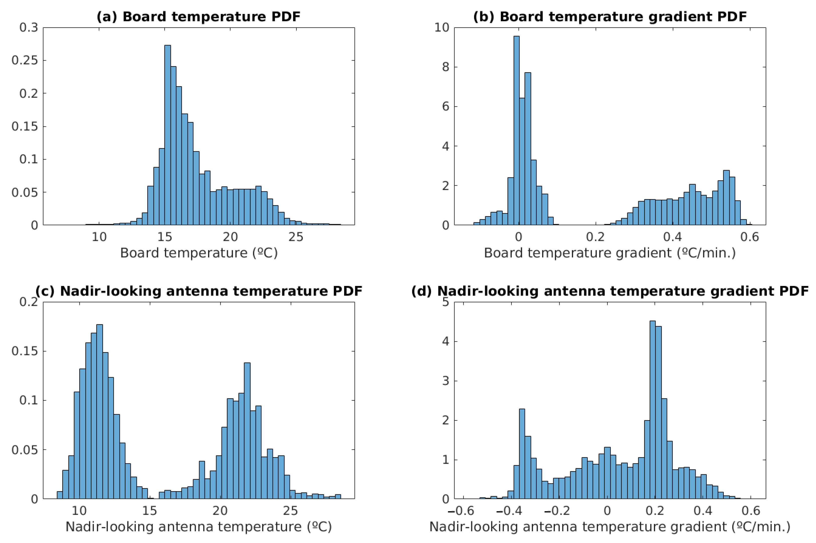
Figure 1 shows four different histograms corresponding to the measured temperatures by the FMPL-2 payload, normalized as a probability density function (PDF). Note that
Figure 1a,c correspond to the measured temperatures in 128 different executions, while
Figure 1b,d correspond to the 1-minute temperature gradient (i.e.,
with
= 1 min). Note that, the temperature gradient of both the instrument board and the antenna are always below 0.6
C/minute, and therefore meeting the instrument requirements. In addition, the temperature range of the instrument is between 10
C and 25
C for both the instrument and the nadir-looking antenna.
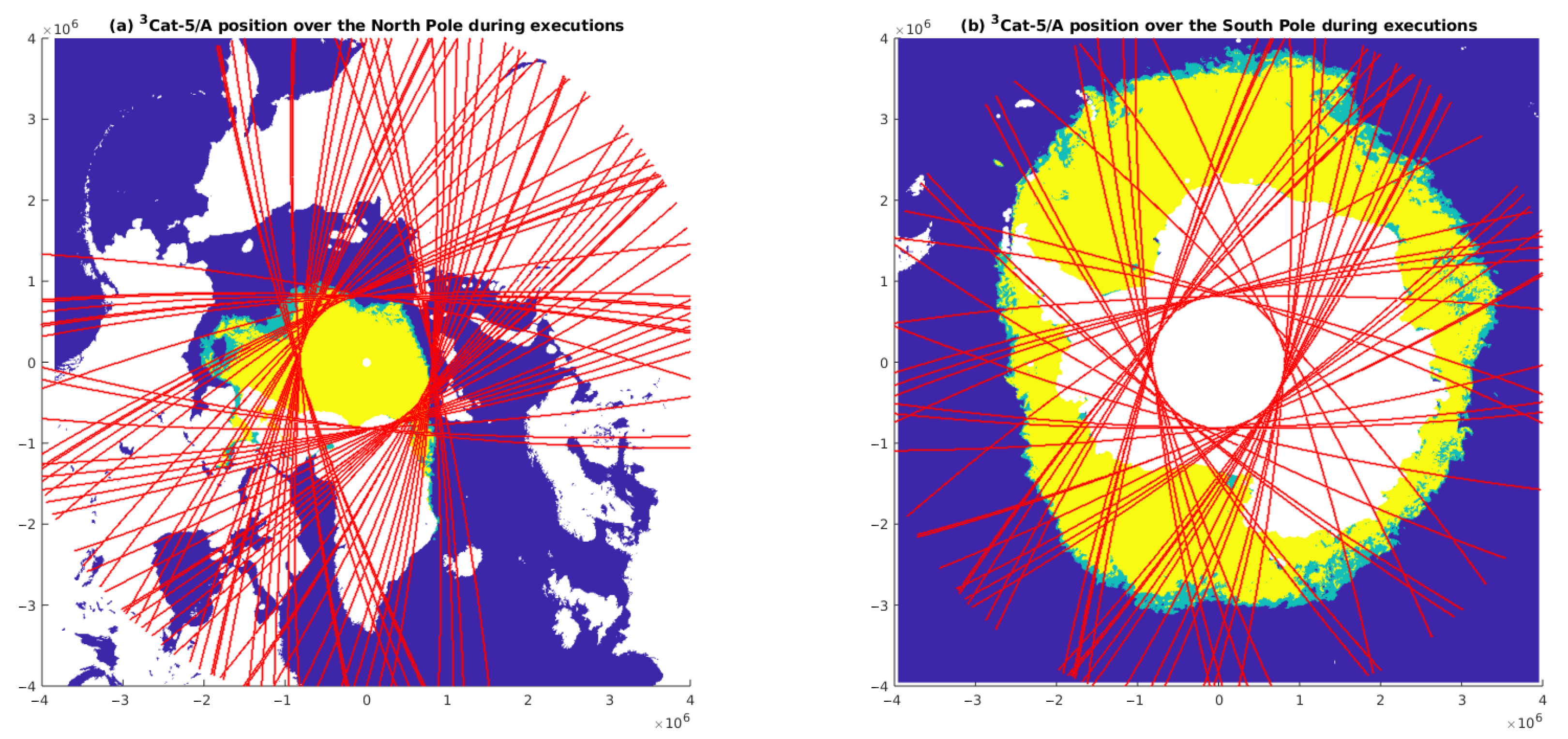
Finally,
Figure 2 shows the different
Cat-5/A tracks (in red) projected using the Lamber-Azimuthal-Equal-Area (LAEA) projection, including the ice extent map (i.e., SIE product from the Satellite Application Facility on Ocean and Sea-Ice (OSISAF) [
34]) on 13 October 2020. The OSISAF SIE product identifies three types of ice depending on the concentration. In
Figure 1, the blue color shows areas without ice concentration (lower than 30%), the light-green area corresponds to open ice (ice concentration between 30% and 70%), and the yellow color identifies closed-ice areas (more than 70% of ice concentration).
3.2. FMPL-2 L-Band Radiometer Review
As introduced in the last section, the temperature knowledge and its stability are crucial for the correct operation of the radiometer. The FMPL-2 radiometer is based on a Total Power Radiometer (TPR) with frequent calibration, integrating 100 ms of data for the antenna, the matched load (ML), and the active cold load (ACL). The process is repeated twice per second. The two main requirements of the instrument are the sensitivity (i.e., radiometric resolution), which shall be lower than 1 K, and the accuracy, which shall be lower than 2 K [
35]. This section presents a summary of the hot and cold load measurements, and the very first geo-located microwave radiometer data for both the North and South poles. Finally, a study of selected stable regions (i.e., middle of the ocean) is presented, which are used to validate both the radiometric sensitivity, and the accuracy of the instrument.
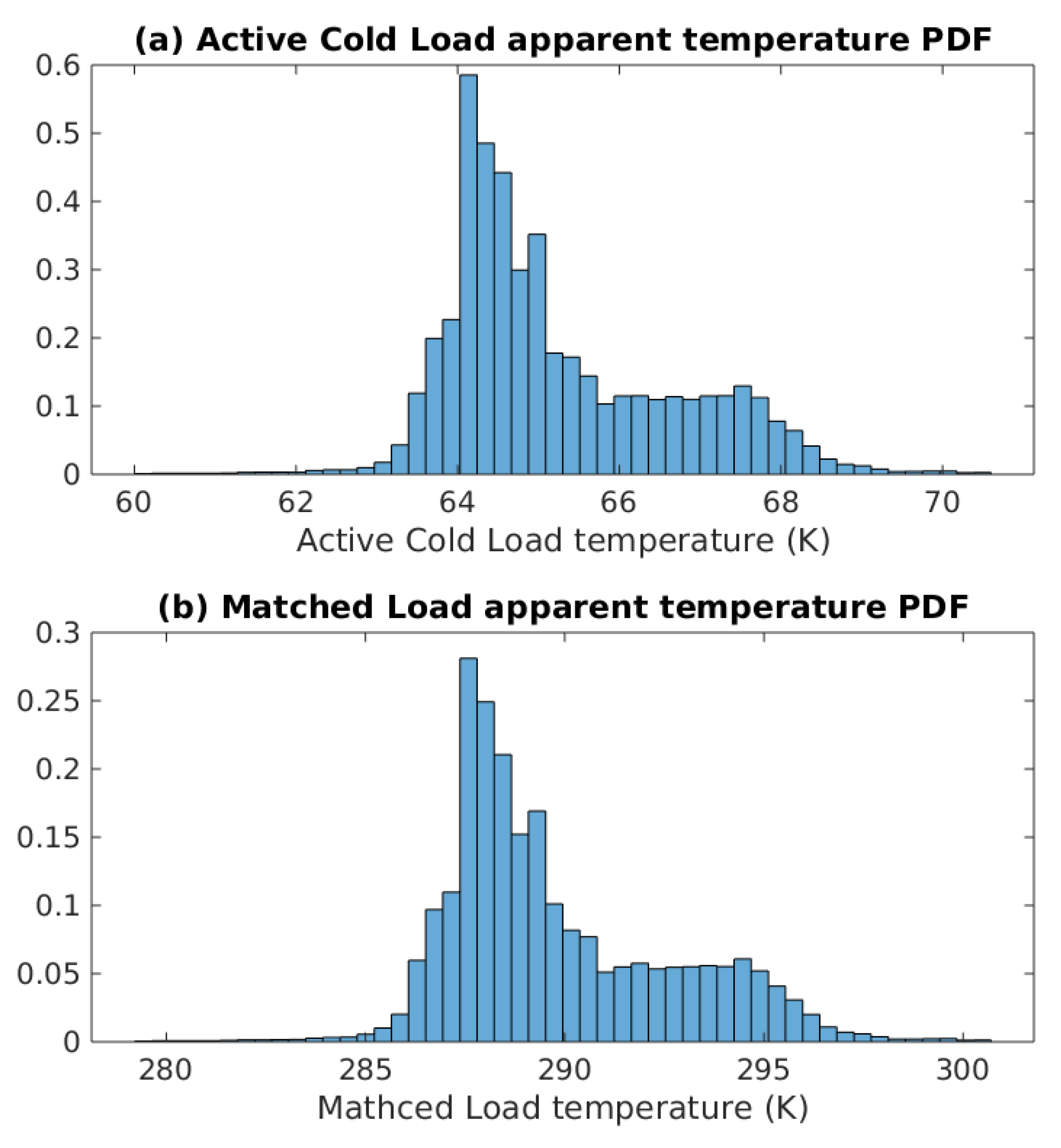
The PDF of the temperature for both internal calibration loads is shown in
Figure 3. As it can be seen, the ML (a 50 Ohm resistor) temperature matches the board temperature (i.e., its noise temperature corresponds to the physical temperature of the component), and the ACL noise measurement has been calibrated for the thermal drifts and switch losses, taking into account the contribution from the ML, as shown in (
1) (Equation (4) from Reference [
31]):
where
dB, the losses input switch, and
and
are the ACL, and the ML noise power measurements.
3.2.1. Measured Antenna Temperature
Once the ancillary data is used to calibrate the radiometer, the final antenna temperature (
) measurement is computed using the instrument gain and bias estimated during the calibration, and finally compensating for the antenna losses, as shown in Equations (4)–(10) of Reference [
31].
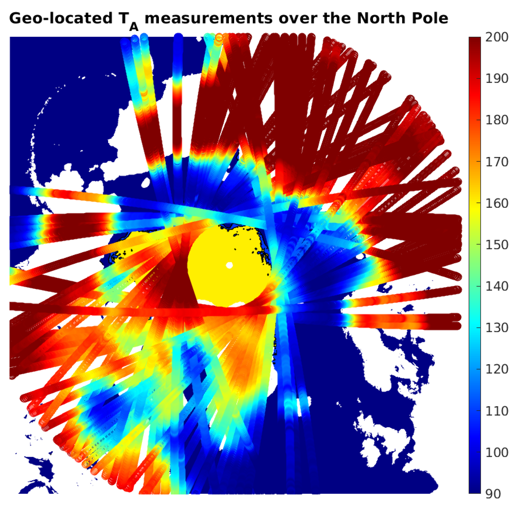
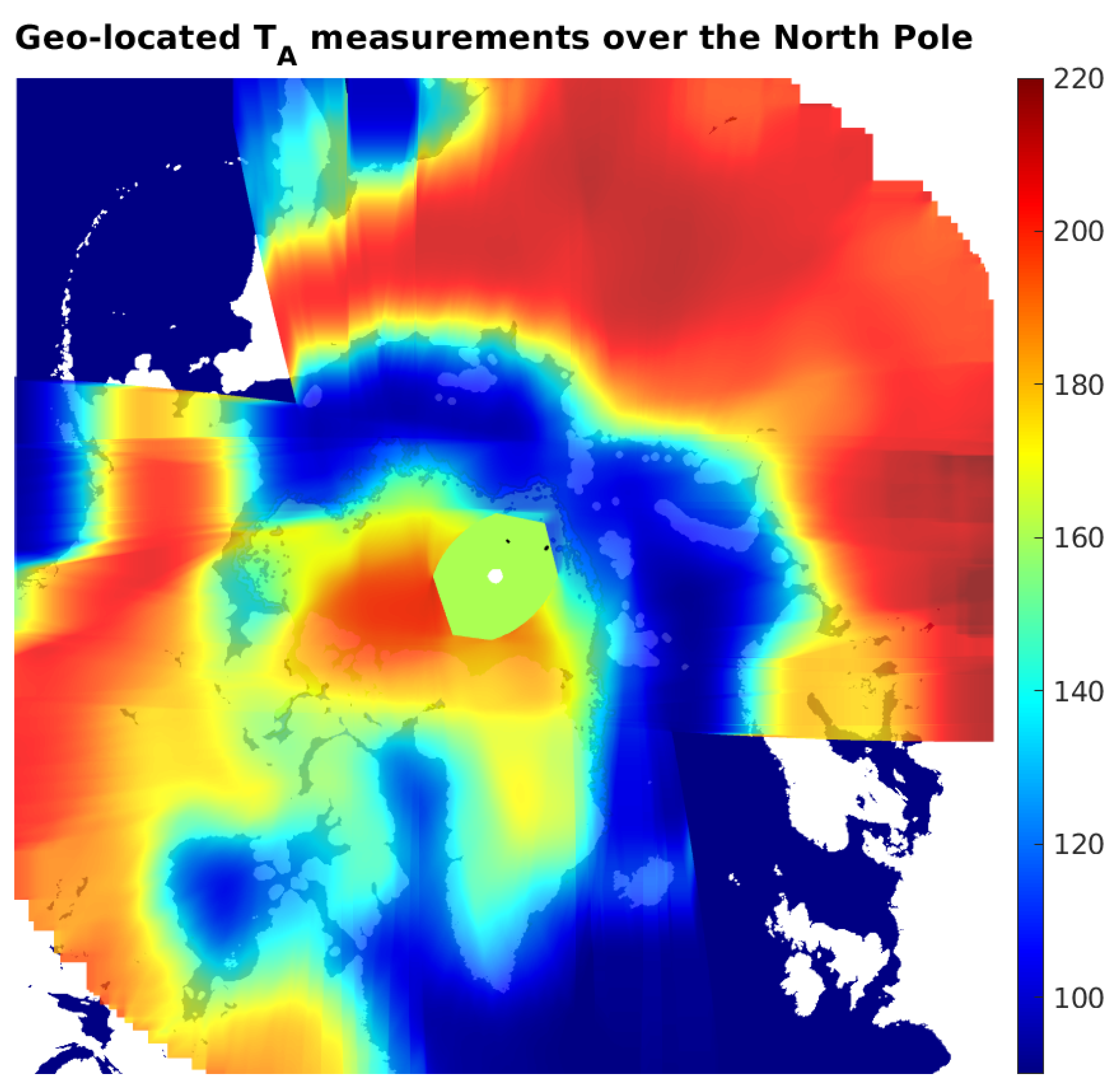
Figure 4 presents 13 days of geo-located FMPL-2 L-band radiometer measurements over the North Pole, for all latitudes above 55
. The geo-located
clearly shows the difference between Land, with a
larger than 180 K; ocean, with an average
90–95 K; and ice, with a
larger than 150 K. It is also remarkable how Greenland and Iceland are identified at the bottom the image. Even though the instrument has a very wide footprint in the cross-track direction (∼580 km), the oversampling (2 Hz) in the along-track direction, and a later co-location of consecutive passes allows to re-construct a 2D image from a number of 1D tracks. Note that, the geo-located images are not projected over a grid yet, and the pixels are not at antenna footprint scale. The ground-truth ice edge data is overlaid below the
track, as it can be seen for latitudes above 86
(dark-yellow), where the S/C cannot measure using the radiometer due to the orbit inclination.
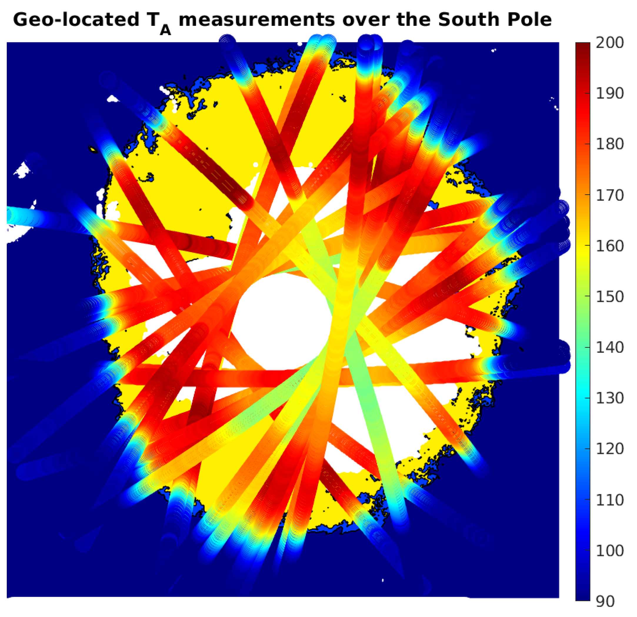
Moreover,
Figure 5 shows the corresponding data for the South Pole, for all latitudes below −55
. Note that, some of the passes of the South Pole show a degraded value of calibrated antenna temperature, which has been identified as a loss of attitude for a given set of orbits. Despite that, it is clearly seen the
gradient in the along-track direction when the S/C enters into the ice, going from 90 K up to ∼180–200 K in a few samples. Thanks to the very high along-track overlapping (∼99%), the sea-ice edge can be accurately estimated by analyzing the gradient of the
evolution, which can then be compared to the tracks of the OSISAF SIE product (in yellow).
As it can be seen in different regions of the image, as in the top right corner or in the bottom left corner, by overlapping different consecutive passes, and assuming the sea-ice edge has not significantly changed between consecutive passes (i.e., separated less than a few days), a 2D reconstructed image of the sea-ice surrounding the Antarctica could be retrieved.
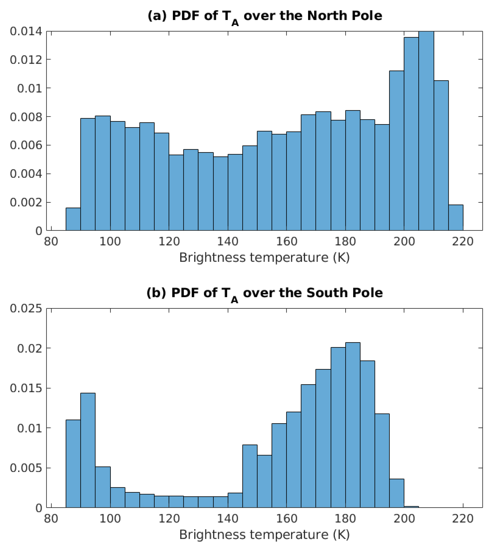
Finally, the PDF of the
for both poles is presented in
Figure 6. As it can be seen in (a), the distribution of antenna temperatures is more evenly distributed than in the South Pole, because in the North Pole images there is a combination of land, water, and different types of ice, with some regions with multiple contributions in the antenna footprint (i.e., Greenland), while in the South Pole there is only ice, land completely covered by ice/snow, and water, with well defined boundaries in the along-track direction of the measurements.
3.2.2. Radiometric Accuracy
As introduced at the beginning of this section, the L-band radiometer has been designed to provide an absolute accuracy better than 2 K. To validate this requirement, the following scenarios are selected:
A track in the Arctic Ocean over water, with enough separation from any land body, or sea-ice, on the 4th of October at 20 UTC, and
A track in the Antarctic ocean before entering into the Antarctica on 1st October 2020 at 18 UTC.
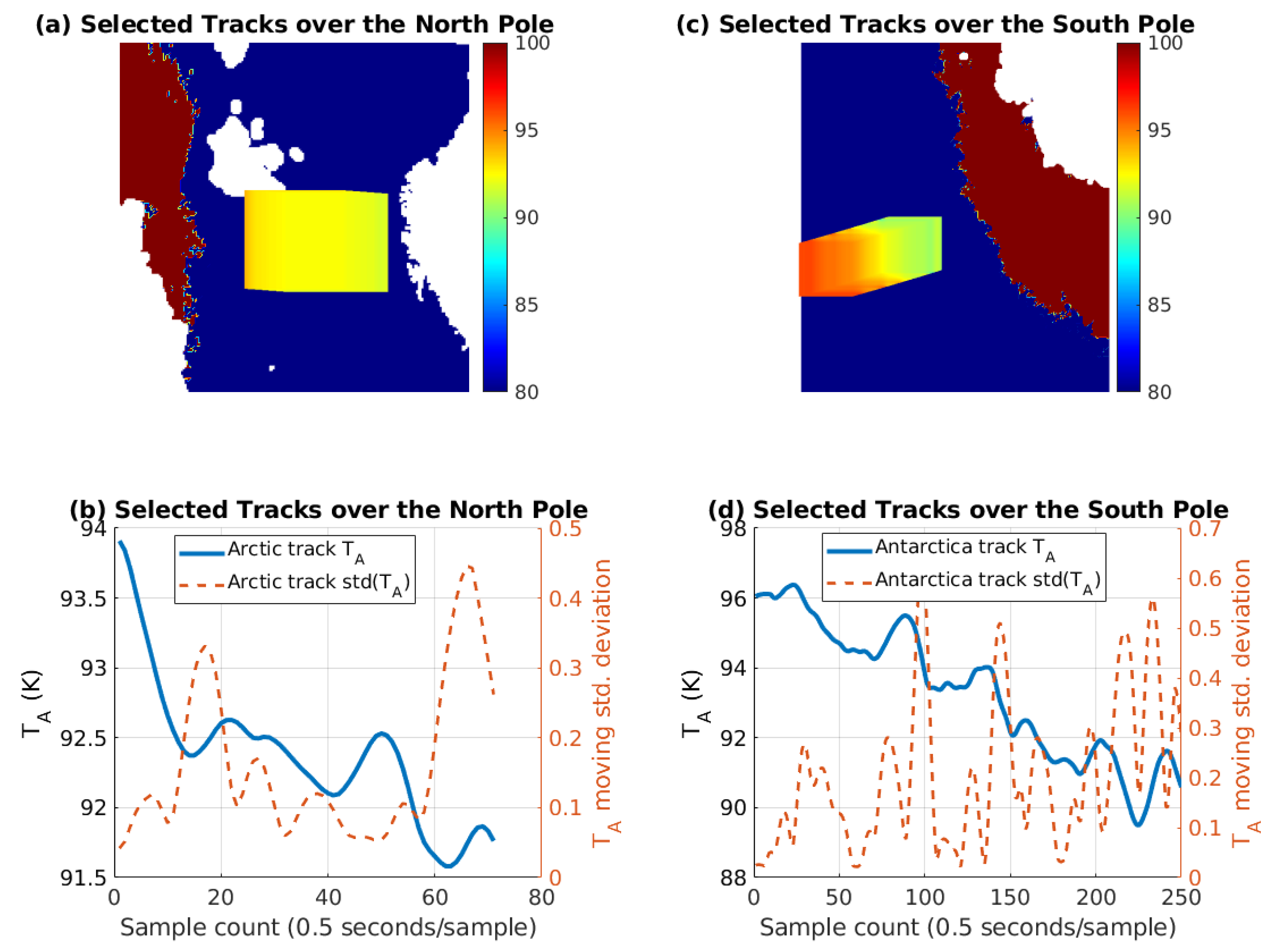
The two selected tracks are shown in
Figure 7. Note that both the geo-located version, and the time-series evolution of the
are presented. Furthermore, a 5-s window (10 samples) standard deviation is presented, together with the time series evolution. The following list summarizes the ground-truth data generated by the ICON model [
36], and downloaded through [
37] for the regions under study:
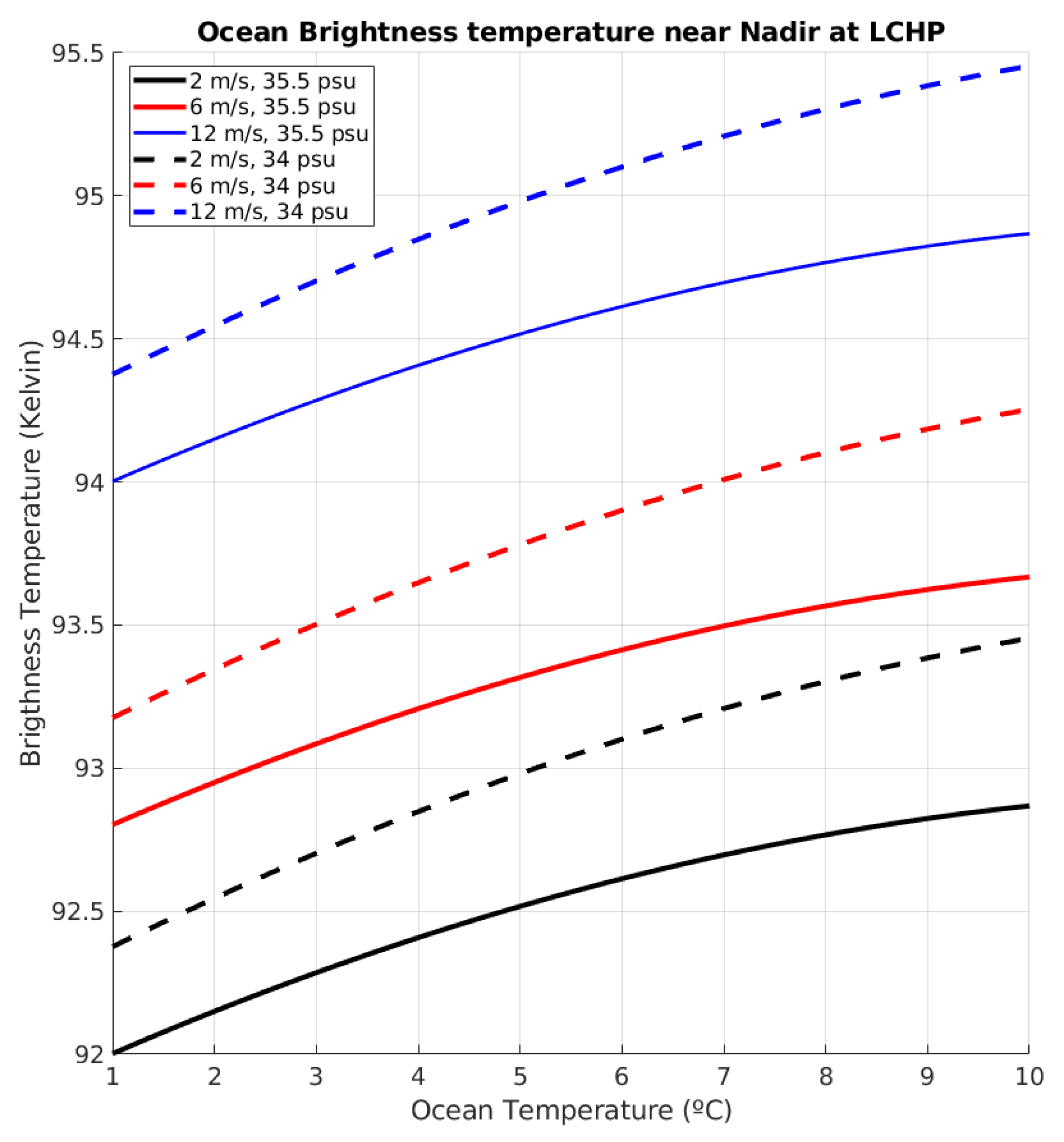
Figure 9 shows the expected brightness temperatures for each combination of salinity, temperature, and wind speed.
The Arctic track
(
Figure 7a,b) is first of all decreasing from ∼94 K rapidly to ∼92.5 K, because the antenna footprint is still collecting some portion of Svalbard. From this point, around sample count 15, the measurements are less noisy, maintaining the measurement ∼92–92.5 K during ∼30 s. Comparing it with
Figure 9, the actual measurement corresponds to the blue curve (∼2 m/s wind) at ∼4
C, therefore the absolute accuracy of this measurement is estimated to be under ∼0.5 K.
Moreover, the same curve is presented for
in
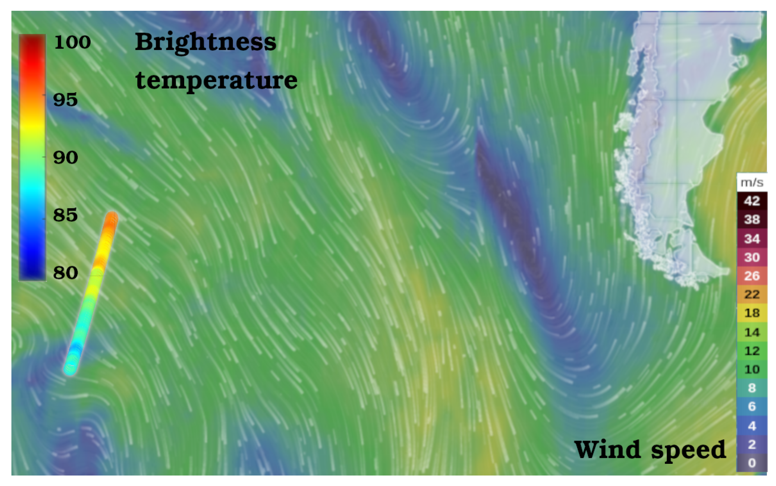
Figure 7c and d for the Antarctica track. In this case, and as shown in
Figure 8, the measurement starts in a very windy area, with winds going from 15 m/s down to 12 m/s. The brightness temperature out of this area is high ∼96 K, which corresponds to high winds (>12 m/s). Despite that, as the satellite moves towards the Antarctica, it enters into a very calm area, with wind speeds ranging from 2–4 m/s, and therefore the received
significantly changes from 96 K down to 92 K, providing in this case an accuracy better than 2 K along the overall time series.
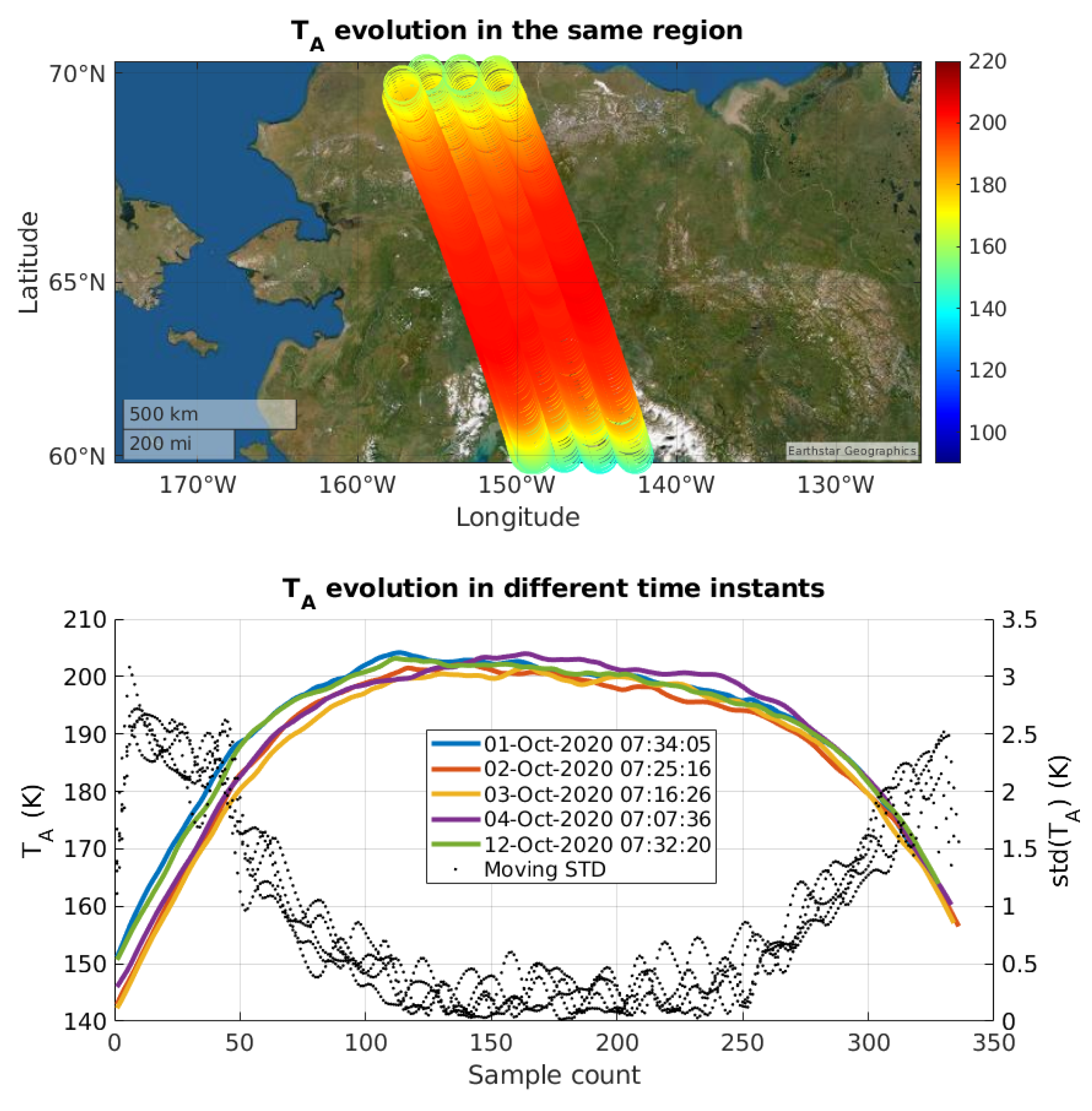
Finally, the instrument shall be stable among consecutive measurements. To validate this stability, five consecutive tracks over the same regions have been selected in the region of Alaska. Four consecutive tracks have been selected, with a separation of one day between them. In addition, a fifth acquisition one week apart has been selected.
Figure 10 shows the evolution of those tracks. As it can be seen, blue (1 October 2020) and green (12 October 2020) tracks are coincident (i.e., the footprint over the same exact region), and both are showing the same evolution, with a mean square error between both at the central part (i.e., between samples count 100 and 250) of 0.34 K. The central point of each of the four consecutive tracks is separated a longitude of ∼2.2
or ∼100 km, which corresponds to an 82% of overlapping in the cross-track direction.
3.2.3. Radiometric Sensitivity
In order to check the radiometric sensitivity, the same scenarios as in the previous section are used. In this case, the radiometer has been designed to provide a sensitivity better than 1 K. The moving standard deviation of
is computed over regions that are apparently stable, as in the middle of the image of
Figure 7c (from samples 20 to 60), and in the land part (from samples 150 to 250) of
Figure 10. In both images, the moving standard deviation of
is below 1 K. In the first case, this magnitude is below 0.2 K, as the ocean is pretty stable with very low speed winds. However, for the land case, the sensitivity in the center of the figure goes up to ∼0.5 K. This behavior is the expected, as on one hand, land is rougher, and less homogeneous. The antenna footprint collects multiple contributions from different sources (i.e., different soil moisture values or vegetation changes), as compared to a calmed and open water. On the other hand, the sensitivity of a TPR depends on the measured
, as shown in Equation (2) from Reference [
31], and therefore the higher the measured
, the higher the sensitivity value.
3.2.4. 2D Image Reconstruction
The overlapping in the cross-track direction (i.e., after 13 days of measurements), allows to compose 2D images, such as the Arctic Ocean one shown in
Figure 11. As it can be seen, two weeks of data allows not only to fill all data gaps over the pole, but also to have enough overlapping in the cross-track direction to reconstruct a 2D image. To reconstruct the image, each measurement is aggregated into a 3 km grid taking into account the antenna footprint (i.e., 580 km in the cross-track and 380 km in the along track). Finally, measurements laying in the same pixel after multiple orbits are averaged. Thanks to the overlap in the cross-track direction, most of the pixels composing a single 1D track are averaged with other 1D tracks, and therefore forming the 2D image with a higher resolution.
To conclude the L-band radiometry review section, it is important to remark that the requirements of the instrument have been successfully achieved, providing an accuracy below 2 K and a sensitivity lower than 1 K. In addition, the measurement drift between consecutive orbits has been quantified, showing negligible drift between consecutive tracks (<0.34 K in 12 days) with an overlap of 82%. Finally, the instrument along-track axis oversampling allows to detect the ice edge and to compose 2D images over a 3 km grid.
3.3. FMPL-2 GNSS-R Review
The second part of the instrument is a GNSS-Reflectometer. The presented data is for the same period of the radiometer, and some selected tracks are presented for GPS L1 C/A case. This part of the instrument works by received GNSS reflections that are produced in either the ocean, the land, or the sea-ice. On contrary to other GNSS-R instruments [
5,
38], the instrument was designed with a maximum incoherent integration time of
ms to avoid the need to retrack in orbit [
14,
39] to avoid blurring of the DDMs [
12], and to increase the spatial resolution. In this case, the spacecraft ground-track velocity is equal to the size of the 1st Fresnel zone (i.e., ∼6.5 km/s ground-track at 40 ms = 250 m), and therefore the spatial resolution of the measurement is the one of the GPS L1 C/A chip (∼300 m). Current GNSS-R spaceborne instrument as SGR-ReSi [
26] on board CyGNSS are working with an integration time of 1s, providing a lower spatial resolution of ∼6.5 km.
In order to review the capabilities of FMPL-2 to receive GNSS reflected signals with such high spatial resolution, several examples are provided over ice, ocean, and land. It is important to mention that all presented tracks have been processed to check that the absolute Doppler of the reflected signal is consistent with the expected one [
40], and that the on-board processor is correctly tracking a GNSS reflection, and not a peak induced by speckle noise or the direct signal. The instrument implements a Parallel Code Phase Search (PCPS) [
41], and therefore all acquisitions are centered into an absolute Doppler shift, and then all code-delays are computed (more details on the FMPL-2 acquisition strategy can be found in Reference [
31], Section II). For this reason, it is crucial to check and filter any track that does not have the expected Doppler shift. Finally, all presented tracks show the geo-located Signal-to-Noise Ratio (SNR), the evolution of the received power, and a DDM time series evolution. The received power is computed as in Reference [
31], Section IV, and all DDMs are all normalized to have the peak equal to 1, and the estimated noise power is subtracted from them to ease its visualization.
3.3.1. Short Integration Time Limitations
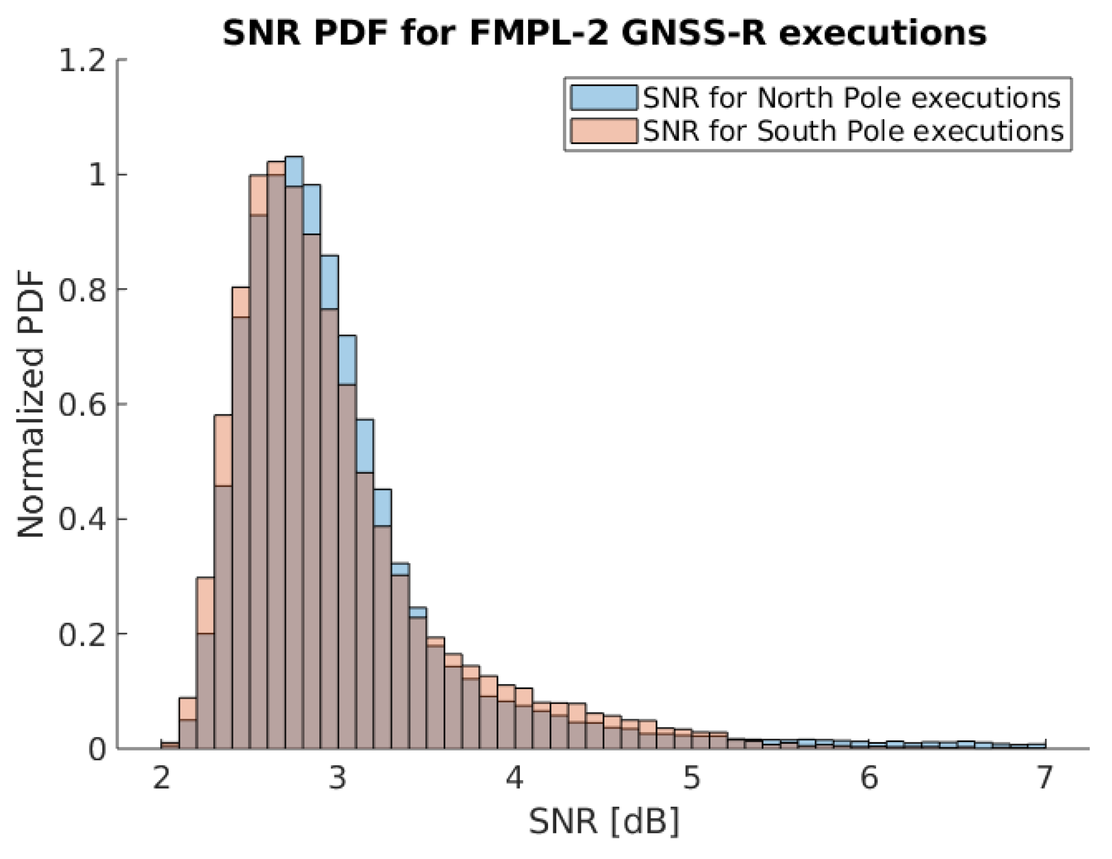
While the very short incoherent integration time avoids tracking of the DDM peak on board, it limits our capability to collect only reflections that are almost specular, and with moderate-high SNR. As opposed to most common-seen DDMs [
13], which are based on 1-s integration, FMPL-2 DDMs cannot reproduce the “famous” horseshoe-shaped DDMs, because tails are blurred in noise.
As it will be presented in the next section for the FMPL-2 case, sea-ice to ocean transitions can be easily identified as a loss of signal tracking, because of this very short integration time, as the signal over the oceans gets blurred under the noise floor. Despite that, as detailed in
Figure 12, the distribution of SNRs is consistent to what is shown in Reference [
42], where the distribution of SNRs behaves as a Rice distribution, and therefore the retrieved data is consistent with the expected behavior for the selected integration time.
3.3.2. Sea-Ice/Ocean transition
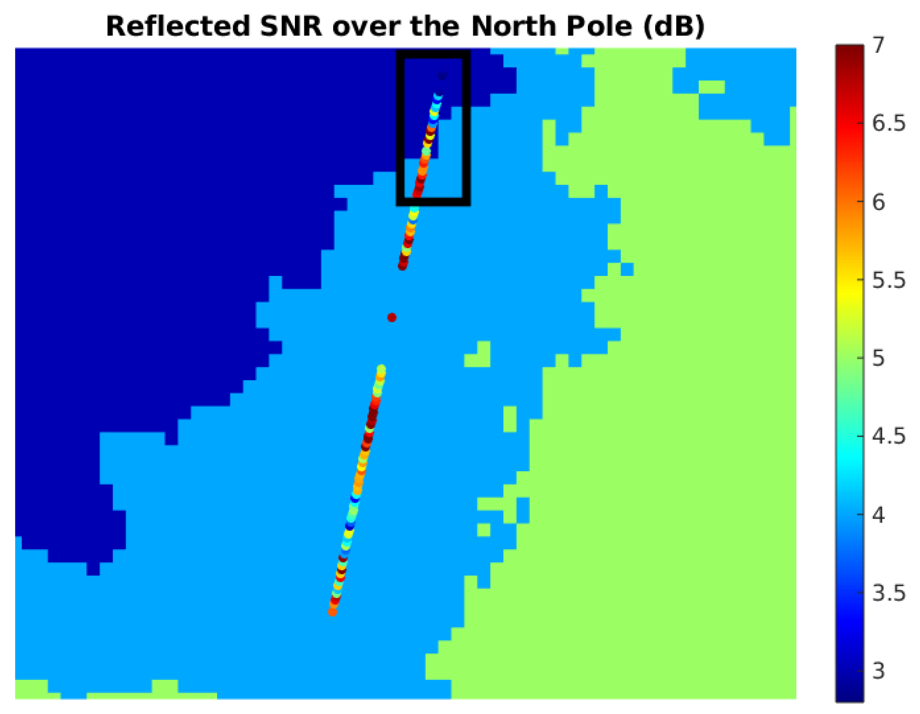
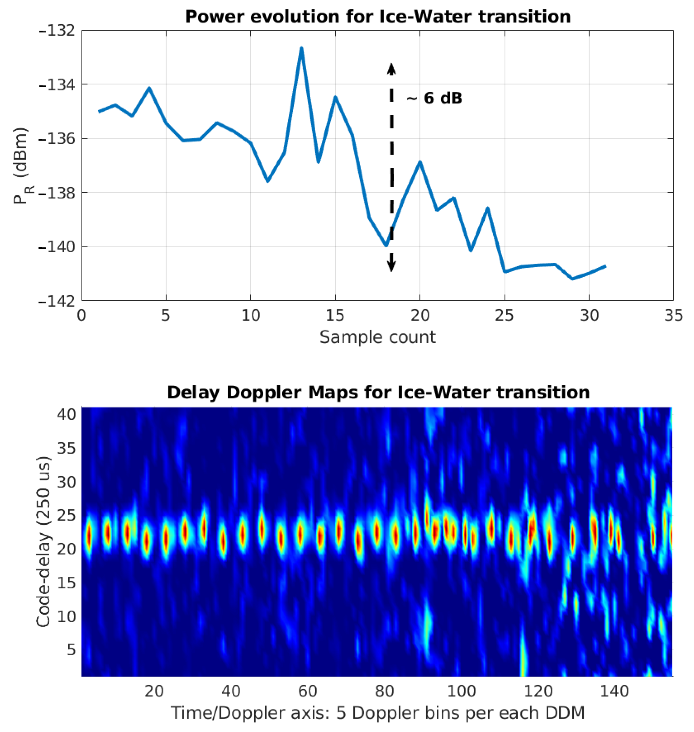
Figure 13 shows the geo-located SNR of a single track collected 6 October 2020, as in other figures, OSISAF SIE is overlaid. Furthermore,
Figure 14 shows a zoom of the boxed data in the top, where the estimated received power
after radiometric calibration is shown. In addition, in the bottom part of the image a set of DDMs is presented, where the X-axis is a combined Doppler-Time axis, composed by 5 Doppler bins (500 Hz) per DDM, and 30 DDMs in total (i.e. X axis goes from 1 to 151), and the Y-axis is the DDM code-delay axis. The incidence angle of this track is ∼33
.
Due to the very short integration time, as the system goes off the sea-ice and enters into the rough ocean, the coherency of the reflected signal decreases, and thus the reflection gets less specular, and the SNR decreases. This can be also identified in the shape of the DDMs, going from a very clear peak (left part of the DDM strip) without Doppler extension, to a noisier observable (in the right part of the DDM strip). As it was introduced in the previous section, this is not a limitation of the instrument, but a design choice to increase the resolution of the SIE products.
3.3.3. Reflections over the Ocean
Despite the fact that specular reflections are not likely to occur, under certain conditions [
43], such as low elevation angles, receiving a high coherent component is possible.
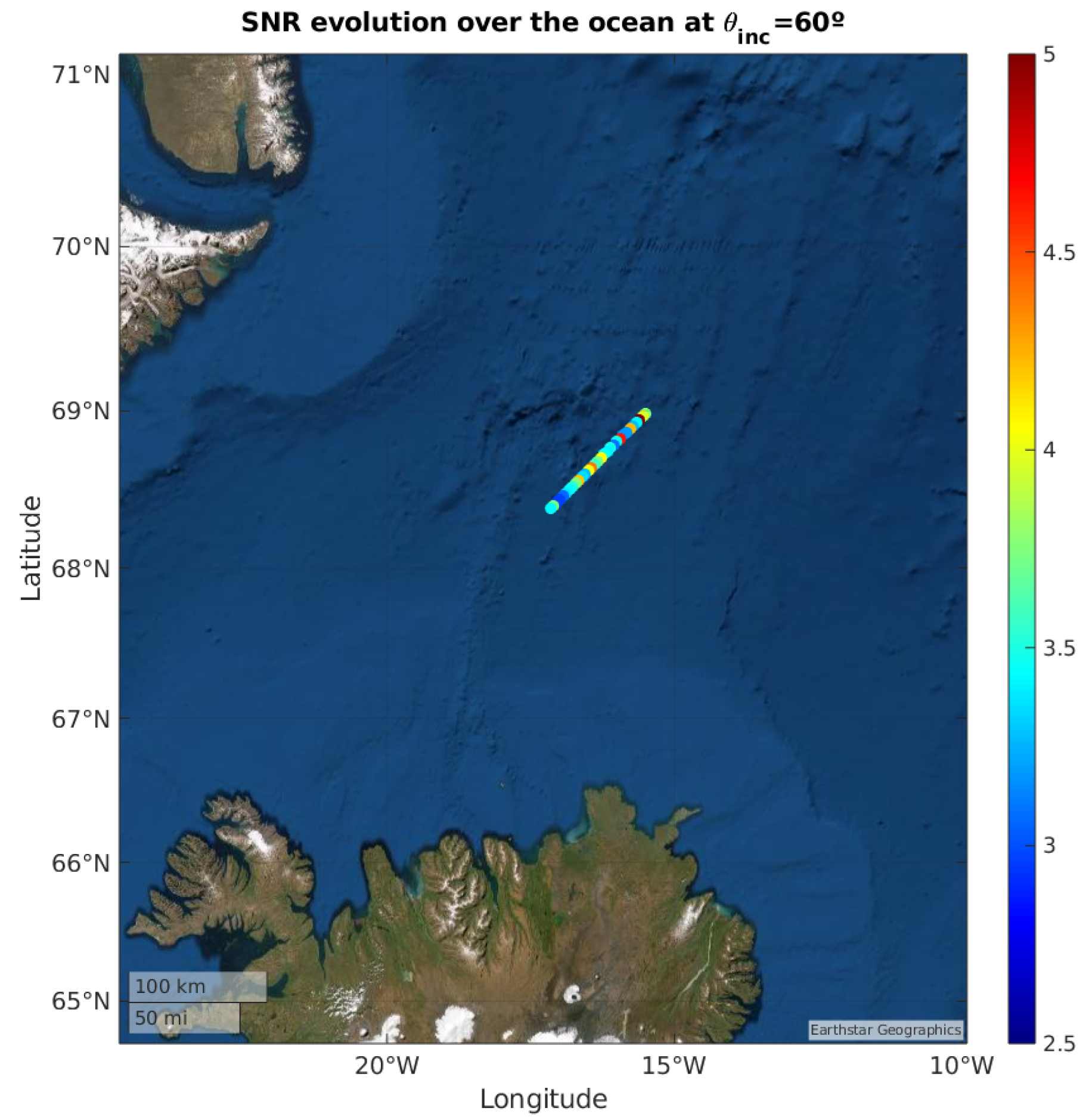
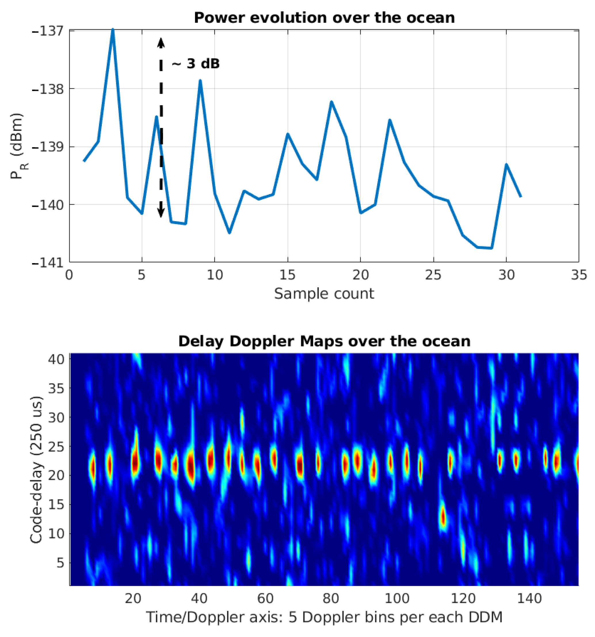
Figure 15 shows a GNSS-R track acquired by FMPL-2 on 10 October 2020, at 16 UTC, containing several consecutive reflections over the ocean, on the area comprised between Iceland and Greenland. The incidence angle of the reflection is ∼60
, and the wind speed data [
37] of the selected region is under 3–4 m/s, and thus it is likely to encounter strong coherent reflections. In the same way as in the first GNSS-R example,
Figure 16 shows both the received power
and the DDM time series evolution with the same Doppler bin space. In this case, the shape of the DDMs is noisier, despite the SNR being larger than 4 dB. However, there is not a notable difference in the DDM shape, mostly because the received reflections are specular.
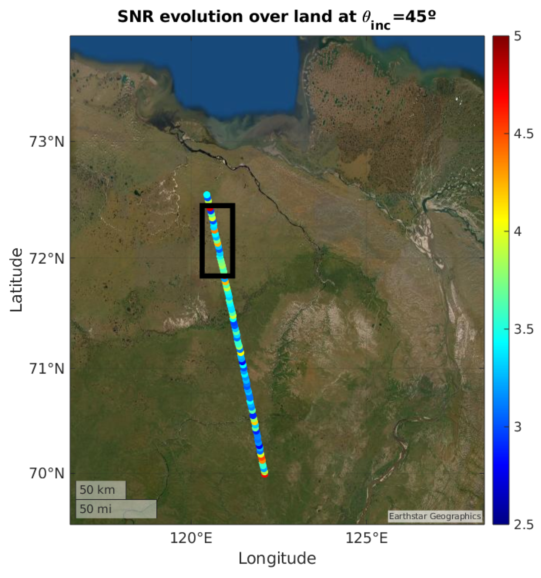
3.3.4. Reflections over Land
To finalize this section, a track has been selected to show the capabilities of FMPL-2 over land, where specular reflections are also more likely to occur [
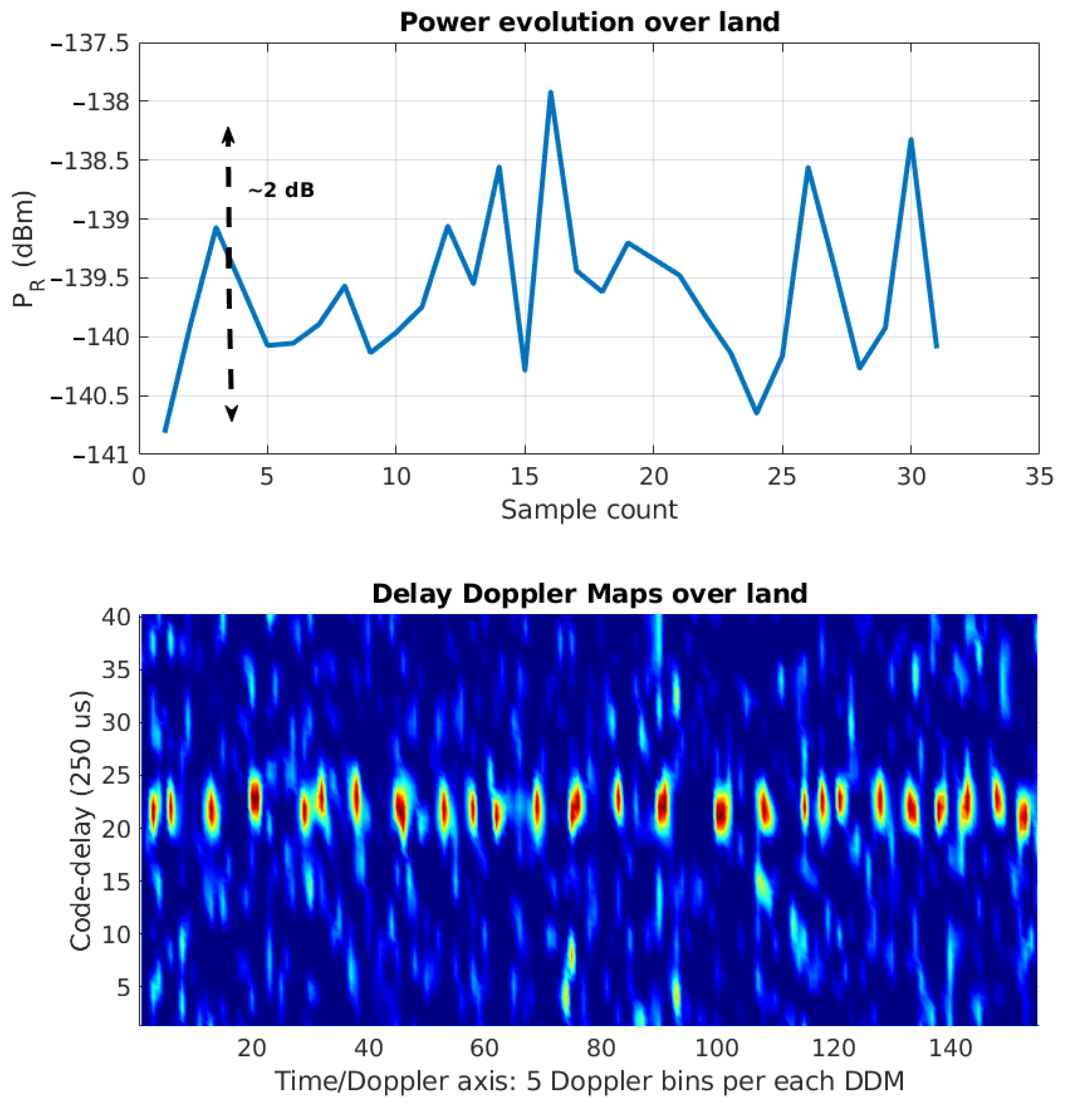
44]. As in the other examples,
Figure 17 and
Figure 18 show the geo-located SNR over the area of interest, the estimated received power
, and the retrived DDMs in the time series format.
In this last case, it can be identified that the overall SNR increases as the track goes towards the North. An increase in the received power that can be linked to either a decrease of the local surface roughness, a decrease of the local vegetation, and an increase of the SM of the measured area. In that case, the area with lower reflectivity is populated with trees, which causes additional attenuation to the reflected signal [
45].
To summarize, this section has presented the capabilities of FMPL-2 to receive GNSS-R data over ice, land, and ocean even using short incoherent integration times. The shorter integration times allows to have an enhanced spatial resolution of ∼300 m, and it has been presented that the sea-ice and ocean transition can be detected as a change in the GNSS-R reflectivity. Moreover, thanks to the selected incoherent integration time, it is easier to calibrate the reflectivity measurements, as most reflections just have contributions from the first Fresnel zone (i.e., ∼300 m), and thanks to the internal radiometric calibration used for the L-band radiometer, the noise power of the instrument can be calibrated. Therefore, the DDM noise power can be calibrated and an absolute radiometric measurement can be provided for each GNSS reflection.
4. Discussion and Potential Applications
We are now living in the big data era, new algorithms are being developed, and neural networks are a good example of simple algorithms with multiple inputs being able to construct valuable outputs. One of the main requirements of this algorithms is to provide large amounts of data points to the algorithm. The use of multiple distributed satellite sensors, such as a CubeSat constellation based on FMPL-2 instruments, will be able to bring this large amount of points, providing lots of measurements both in space and time at a reduced cost, as compared to a big satellite approach.
Moreover, following the concept introduced in Reference [
46], in the paradigm of a CubeSat-based constellation for Earth Observation based on FMPL-2, the improvement on the spatial resolution could be achieved by adding more spacecrafts into the system, as in the CyGNSS constellation. Multiple satellites can provide a larger overlap in the cross-track direction, which is one of the limiting factors of the FMPL-2 antenna footprint. However, the implementation of such a system needs to cope with a large network deployment, as pointed out by Reference [
47]. Despite being easier to replace or develop than larger satellites, managing a large constellation without the support of a well-structured network underneath is a titanic task.
Furthermore, and both in a single-spacecraft configuration or in a constellation, FMPL-2 the geo-location of consecutive FMPL-2 executions allow to reconstruct 2D images from 1D tracks, and by just adding more
sensors to an hypothetical constellation, the revisit time can be lowered, and the spatial resolution of the observations enhanced. This concept was introduced by Reference [
46] for GNSS-R constellations, but it is also applicable to the L-band radiometer case, as in FMPL-2, where a 580 km pixel can be averaged out of multiple measurements from different CubeSats.
Aside from the potential that this type of instruments have in CubeSat constellations, FMPL-2 by itself in a single-spacecraft configuration is able to retrieve valuable geophysical parameters. It has been shown that the L-band radiometric measurements are matching the sea-ice extent product of OSISAF, and that GNSS-R reflectivity measurements are also sensitive the ice extent. Moreover, FMPL-2 has prove its capabilities to detect wind speed over the ocean from brightness temperature variations. Furthermore, the increase of brightness temperature over the permafrost ice in the Arctic Sea shows that the sensor is also sensitive to ice thickness variations. In addition, the abrupt increase in the brightness temperature in the along-track direction when approaching the sea-ice (i.e., in the Antarctic ocean) allows to precisely determine the sea-ice edge border.
In addition, the combination of L-band measurements and multiple GNSS-R tracks into single pixel may open the potential of down-scaling the final FMPL-2 observable. The combination of a high-resolution and a low-resolution sensor would allow to provide down-scale the resolution of MWR maps, and thanks to state-of-the-art algorithms, such as neural networks, it can be achieved. In this case, the performance of a very low resolution instrument (radiometer) can be improved with a high resolution instrument (GNSS-R), where the MWR fills the spatial gaps between GNSS-R measurements.
To conclude, the formation of FMPL-2 images from the combination of consecutive and the use of advanced algorithms would allow to reconstruct 2D maps of high-interest geophysical product, such as SIE, SIT, or Soil Moisture, and in order to increase its spatial resolution or revisit time, it would be as easy as adding a new CubeSat with another FMPL-2, just as Planet Labs or Spire are actually doing.
5. Conclusions
This work has presented the validation of the FMPL-2, a dual microwave (GNSS-R and MWR) instrument on board the FSSCat mission. After the commissioning of the instrument, the measurements provided in the first weeks of October 2020 have been used to validate the mission requirements. It has also been proven that the high oversampling of the radiometer footprint in the along-track direction allows to generate preliminary brightness temperature maps, where its match with the OSISAF SIE product can be identified. Finally, three different tracks of GNSS reflections have been presented, over ice, ocean, and land, showing the performance of GNSS-R even using short (40 ms) incoherent integration times.
Author Contributions
Conceptualization, J.F.M.-M., L.F., A.C., B.C.D., and M.P.; methodology, J.F.M.-M., L.F., A.P., J.A.R.-d.-A., and A.C.; software, J.F.M.-M., A.P., J.A.R.-d.-A., and H.P.; validation, A.C.; formal analysis, J.F.M.-M., H.P., and A.C.; investigation, J.F.M.-M. and A.C.; resources A.C., B.C.D., M.P., and M.P.; data curation J.F.M.-M. and A.C.; visualization J.F.M.-M.; supervision A.C., B.C.D., and M.P.; project administration A.C., B.C.D., and M.P.; funding acquisition, A.C., B.C.D., and M.P.; writing—original draft preparation, J.F.M.-M. and A.C.; writing—review and editing, J.F.M.-M., A.P., H.P., A.C., B.C.D., and M.P. All authors have read and agreed to the published version of the manuscript.
Funding
This work was supported by 2017 ESA S3 challenge and Copernicus Masters overall winner award (“FSSCat” project). this work has been (partially) sponsored by project SPOT: Sensing with Pioneering Opportunistic Techniques grant RTI2018-099008-B-C21/AEI/10.13039/501100011033, and by the Unidad de Excelencia Maria de Maeztu MDM-2016-0600, and by the ICREA Academia award by the Generalitat de Catalunya, and by the grant for recruitment of early-stage research staff FI-DGR 2018 of the AGAUR—Generalitat de Catalunya (FEDER), Spain.
Institutional Review Board Statement
Not applicable.
Informed Consent Statement
Not applicable.
Data Availability Statement
Data used in this study will be publicly and freely available for everyone at the Copernicus system as part of the FSSCat mission.
Acknowledgments
The authors would like to thank all NanoSat-Lab members who made possible the development and testing of the FMPL-2 payload, as well the support to build Montsec S-band ground station used to download FMPL-2 data. The authors would like to thank Balamis S.L. employees Roger Jové, Adrià Amezaga, and Ricard Gonzálvez who designed and manufactured the RF front-end board of FMPL-2 with the internal calibrators. The authors would also like to thank Tyvak International operations Blue, Orange, and Green teams, specially Alessio Piumatti, Filippo Corradino, and Rafaelle Mozzillo for their support during FMPL-2 commissioning. The authors would like to thank Miriam Pablos for her support with the generation of SMOS ground truth data.
Conflicts of Interest
The authors declare no conflict of interest.
References
- Arianespace. Vega Flight VV16 Launch Kit (PDF). Available online: https://www.arianespace.com/wp-content/uploads/2020/06/VV16-launchkit-EN3.pdf (accessed on 3 September 2020).
- Camps, A.; Golkar, A.; Gutierrez, A.; de Azua, J.R.; Munoz-Martin, J.; Fernandez, L.; Diez, C.; Aguilella, A.; Briatore, S.; Akhtyamov, R.; et al. Fsscat, the 2017 Copernicus Masters’ “Esa Sentinel Small Satellite Challenge” Winner: A Federated Polar and Soil Moisture Tandem Mission Based on 6U Cubesats. In Proceedings of the IGARSS 2018—2018 IEEE International Geoscience and Remote Sensing Symposium, Valencia, Spain, 22–27 July 2018. [Google Scholar] [CrossRef]
- Cosine Measurement Systems. Hyperscout from Cosine Website. Available online: https://hyperscout.nl/ (accessed on 1 December 2018).
- Ruf, C.S.; Gleason, S.; Jelenak, Z.; Katzberg, S.; Ridley, A.; Rose, R.; Scherrer, J.; Zavorotny, V. The CYGNSS nanosatellite constellation hurricane mission. In Proceedings of the 2012 IEEE International Geoscience and Remote Sensing Symposium, Munich, Germany, 22–27 July 2012; pp. 214–216. [Google Scholar] [CrossRef]
- eoPortal Directory. Cyclone GNSS Mission Description Website. Available online: https://directory.eoportal.org/web/eoportal/satellite-missions/c-missions/cygnss (accessed on 20 January 2019).
- Peral, E.; Tanelli, S.; Statham, S.; Joshi, S.; Imken, T.; Price, D.; Sauder, J.; Chahat, N.; Williams, A. RainCube: The first ever radar measurements from a CubeSat in space. J. Appl. Remote Sens. 2019, 13, 1–13. [Google Scholar] [CrossRef]
- Blackwell, W.J. Radiometer development for small satellite microwave atmospheric remote sensing. In Proceedings of the 2017 IEEE International Geoscience and Remote Sensing Symposium (IGARSS), Fort Worth, TX, USA, 23–28 July 2017; pp. 267–270. [Google Scholar] [CrossRef]
- Misra, S.; Brown, S.; Jarnot, R.; Felten, C.; Bendig, R.; Kocz, J.; McKelvey, C.; Ball, C.; Chen, C.; O’Brien, A.; et al. CubeSat Radiometer Radio Frequency Interference Technology (CubeRRT) Validation Mission: Enabling Future Resource-Constrained Science Missions. In Proceedings of the IGARSS 2018—2018 IEEE International Geoscience and Remote Sensing Symposium, Valencia, Spain, 22–27 July 2018; pp. 6308–6311. [Google Scholar] [CrossRef]
- Reising, S.C.; Gaier, T.C.; Kummerow, C.D.; Padmanabhan, S.; Lim, B.H.; Brown, S.T.; Heneghan, C.; Chandra, C.V.; Olson, J.; Berg, W. Temporal Experiment for Storms and Tropical Systems Technology Demonstration (TEMPEST-D): Reducing risk for 6U-Class nanosatellite constellations. In Proceedings of the 2016 IEEE International Geoscience and Remote Sensing Symposium (IGARSS), Beijing, China, 10–15 July 2016; pp. 5559–5560. [Google Scholar] [CrossRef]
- Blackwell, W.J.; Braun, S.; Bennartz, R.; Velden, C.; DeMaria, M.; Atlas, R.; Dunion, J.; Marks, F.; Rogers, R.; Annane, B.; et al. An overview of the TROPICS NASA Earth Venture Mission. Q. J. R. Meteorol. Soc. 2018, 144, 16–26. [Google Scholar] [CrossRef]
- Lemur-2. Gunter’s Space Page. Available online: https://space.skyrocket.de/doc_sdat/lemur-2.htm (accessed on 3 November 2020).
- Zavorotny, V.U.; Gleason, S.; Cardellach, E.; Camps, A. Tutorial on Remote Sensing Using GNSS Bistatic Radar of Opportunity. IEEE Geosci. Remote Sens. Mag. 2014, 2, 8–45. [Google Scholar] [CrossRef]
- Foti, G.; Gommenginger, C.; Jales, P.; Unwin, M.; Shaw, A.; Robertson, C.; Roselló, J. Spaceborne GNSS reflectometry for ocean winds: First results from the UK TechDemoSat-1 mission. Geophys. Res. Lett. 2015, 42, 5435–5441. [Google Scholar] [CrossRef]
- Park, H.; Valencia, E.; Camps, A.; Rius, A.; Ribó, S.; Martin-Neira, M. Delay tracking in spaceborne GNSS-R ocean altimetry. IEEE Geosci. Remote Sens. Lett. 2013, 10, 57–61. [Google Scholar] [CrossRef]
- Rius, A.; Nogués-Correig, O.; Ribó, S.; Cardellach, E.; Oliveras, S.; Valencia, E.; Park, H.; Tarongi, J.M.; Camps, A.; van der Marel, H.; et al. Altimetry with GNSS-R interferometry: First proof of concept experiment. GPS Solut. 2012, 16, 231–241. [Google Scholar] [CrossRef]
- Alonso-Arroyo, A.; Zavorotny, V.; Camps, A. Sea Ice Detection Using U.K. TDS-1 GNSS-R Data. IEEE Trans. Geosci. Remote Sens. 2017, 55, 4989–5001. [Google Scholar] [CrossRef]
- Yan, Q.; Huang, W. Sea Ice Remote Sensing Using GNSS-R: A Review. Remote Sens. 2019, 11, 2565. [Google Scholar] [CrossRef]
- Camps, A.; Park, H.; Pablos, M.; Foti, G.; Gommenginger, C.P.; Liu, P.; Judge, J. Sensitivity of GNSS-R Spaceborne Observations to Soil Moisture and Vegetation. IEEE J. Sel. Top. Appl. Earth Obs. Remote Sens. 2016, 9, 4730–4742. [Google Scholar] [CrossRef]
- Camps, A.; Vall·llossera, M.; Park, H.; Portal, G.; Rossato, L. Sensitivity of TDS-1 GNSS-R Reflectivity to Soil Moisture: Global and Regional Differences and Impact of Different Spatial Scales. Remote Sens. 2018, 10, 1856. [Google Scholar] [CrossRef]
- Edokossi, K.; Calabia, A.; Jin, S.; Molina, I. GNSS-Reflectometry and Remote Sensing of Soil Moisture: A Review of Measurement Techniques, Methods, and Applications. Remote Sens. 2020, 12, 614. [Google Scholar] [CrossRef]
- Chew, C.C.; Small, E.E. Soil Moisture Sensing Using Spaceborne GNSS Reflections: Comparison of CYGNSS Reflectivity to SMAP Soil Moisture. Geophys. Res. Lett. 2018, 45, 4049–4057. [Google Scholar] [CrossRef]
- Clarizia, M.P.; Pierdicca, N.; Costantini, F.; Floury, N. Analysis of CYGNSS Data for Soil Moisture Retrieval. IEEE J. Sel. Top. Appl. Earth Obs. Remote Sens. 2019, 12, 2227–2235. [Google Scholar] [CrossRef]
- Al-Khaldi, M.M.; Johnson, J.T.; O’Brien, A.J.; Balenzano, A.; Mattia, F. Time-Series Retrieval of Soil Moisture Using CYGNSS. IEEE Trans. Geosci. Remote Sens. 2019, 57, 4322–4331. [Google Scholar] [CrossRef]
- Carreno-Luengo, H.; Luzi, G.; Crosetto, M. Above-Ground Biomass Retrieval over Tropical Forests: A Novel GNSS-R Approach with CyGNSS. Remote Sens. 2020, 12, 1368. [Google Scholar] [CrossRef]
- Unwin, M.; Gleason, S.; Brennan, M. The Space GPS Reflectometry Experiment on the UK Disaster Monitoring Constellation Satellite. In Proceedings of the 16th International Technical Meeting of the Satellite Division of The Institute of Navigation (ION GPS/GNSS 2003), Portland, OR, USA, 9–12 September 2003; p. 2656. [Google Scholar]
- Unwin, M. The SGR-ReSI Experiment on the TechDemoSat-1 Mission. In Proceedings of the CEOI Technology Conference, Abingdon, UK, 22–24 June 2015. [Google Scholar]
- Gleason, S.; Ruf, C. Overview of the Delay Doppler Mapping Instrument (DDMI) for the cyclone global navigation satellite systems mission (CYGNSS). In Proceedings of the 2015 IEEE MTT-S International Microwave Symposium, Phoenix, AZ, USA, 17–22 May 2015; pp. 1–4. [Google Scholar] [CrossRef]
- Jing, C.; Niu, X.; Duan, C.; Lu, F.; Di, G.; Yang, X. Sea Surface Wind Speed Retrieval from the First Chinese GNSS-R Mission: Technique and Preliminary Results. Remote Sens. 2019, 11, 3013. [Google Scholar] [CrossRef]
- Jales, P.; Esterhuizen, S.; Masters, D.; Nguyen, V.; Correig, O.N.; Yuasa, T.; Cartwright, J. The new Spire GNSS-R satellite missions and products. In Image and Signal Processing for Remote Sensing XXVI; Bruzzone, L., Bovolo, F., Santi, E., Eds.; International Society for Optics and Photonics: Washington, DC, USA, 2020; Volume 11533. [Google Scholar] [CrossRef]
- FSSCat—Towards Federated EO Systems. Available online: https://copernicus-masters.com/winner/ffscat-towards-federated-eo-systems/ (accessed on 29 September 2020).
- Munoz-Martin, J.F.; Capon, L.F.; de Azua, J.A.R.; Camps, A. The Flexible Microwave Payload-2: A SDR-Based GNSS-Reflectometer and L-Band Radiometer for CubeSats. IEEE J. Sel. Top. Appl. Earth Obs. Remote Sens. 2020, 13, 1298–1311. [Google Scholar] [CrossRef]
- Ruiz-de-Azua, J.A.; Garzaniti, N.; Golkar, A.; Calveras, A.; Camps, A. Towards Federated Satellite Systems and Internet of Satellites: The Federation Deployment Control Protocol. IEEE Access 2020. submitted. [Google Scholar]
- Valencia, E.; Camps, A.; Marchan-Hernandez, J.F.; Bosch-Lluis, X.; Rodriguez-Alvarez, N.; Ramos-Perez, I. Advanced architectures for real-time Delay-Doppler Map GNSS-reflectometers: The GPS reflectometer instrument for PAU (griPAU). Adv. Space Res. 2010, 46, 196–207. [Google Scholar] [CrossRef]
- EUMETSAT. Sea Ice Edge Product of the EUMETSAT Ocean and Sea Ice Satellite Application Facility. OSI SAF. Available online: www.osi-saf.org (accessed on 25 October 2020).
- FSSCat Consortia. FSSCat Mission Requirement Document (MRD). Unpublish.
- (DWD), D.W. ICON Model Description by DWD. Available online: https://www.dwd.de (accessed on 7 January 2020).
- InMeteo. Ventusky. Available online: https://ventusky.com (accessed on 7 January 2020).
- Jales, P. Spaceborne Receiver Design for Scatterometric GNSS Reflectometry. Ph.D. Thesis, University of Surrey, Guildford, UK, 2012. [Google Scholar]
- Camps, A.; Park, H.; Valencia i Domenech, E.; Pascual, D.; Martin, F.; Rius, A.; Ribo, S.; Benito, J.; Andres-Beivide, A.; Saameno, P.; et al. Optimization and Performance Analysis of Interferometric GNSS-R Altimeters: Application to the PARIS IoD Mission. IEEE J. Sel. Top. Appl. Earth Obs. Remote Sens. 2014, 7, 1436–1451. [Google Scholar] [CrossRef]
- Park, H.; Pascual, D.; Camps, A.; Martin, F.; Alonso-Arroyo, A.; Carreno-Luengo, H. Analysis of Spaceborne GNSS-R Delay-Doppler Tracking. IEEE J. Sel. Top. Appl. Earth Obs. Remote Sens. 2014, 7, 1481–1492. [Google Scholar] [CrossRef]
- Khan, R.; Khan, S.U.; Zaheer, R.; Khan, S. Acquisition strategies of GNSS receiver. In Proceedings of the International Conference on Computer Networks and Information Technology, Bara Gali, Abbottabad District, Pakistan, 11–13 July 2011; pp. 119–124. [Google Scholar] [CrossRef]
- Ferre-Lillo, P.; Rodriguez-Alvarez, N.; Bosch-Lluis, X.; Valencia, E.; Marchan-Hernandez, J.; Camps, I.R.P.A. Delay-Doppler Maps study over ocean, land and ice from space. In Proceedings of the 2009 IEEE International Geoscience and Remote Sensing Symposium, Cape Town, South Africa, 12–17 July 2009. [Google Scholar] [CrossRef]
- Balakhder, A.M.; Al-Khaldi, M.M.; Johnson, J.T. On the Coherency of Ocean and Land Surface Specular Scattering for GNSS-R and Signals of Opportunity Systems. IEEE Trans. Geosci. Remote Sens. 2019, 57, 10426–10436. [Google Scholar] [CrossRef]
- Camps, A. Spatial Resolution in GNSS-R Under Coherent Scattering. IEEE Geosci. Remote Sens. Lett. 2019, 17, 32–36. [Google Scholar] [CrossRef]
- Camps, A.; Park, H.; Castellví, J.; Corbera, J.; Ascaso, E. Single-Pass Soil Moisture Retrievals Using GNSS-R: Lessons Learned. Remote Sens. 2020, 12, 2064. [Google Scholar] [CrossRef]
- Bussy-Virat, C.D.; Ruf, C.S.; Ridley, A.J. Relationship Between Temporal and Spatial Resolution for a Constellation of GNSS-R Satellites. IEEE J. Sel. Top. Appl. Earth Obs. Remote Sens. 2019, 12, 16–25. [Google Scholar] [CrossRef]
- Ruiz-De-Azua, J.A.; Calveras, A.; Camps, A. A Novel Dissemination Protocol to Deploy Opportunistic Services in Federated Satellite Systems. IEEE Access 2020, 8, 142348–142365. [Google Scholar] [CrossRef]
Figure 1.
(a) Temperature probability density function (PDF) of the instrument board during executions, (b) 1-minute integrated temperature gradient of the instrument board, (c) Temperature PDF of the nadir-looking antenna during executions (d) 1-minute integrated temperature gradient of the nadir—looking antenna.
Figure 2.
(a) North Pole tracks of FMPL-2 executions in LAEA coordinates, and (b) South Pole tracks of FMPL-2 executions in LAEA coordinates. Both figures with OSISAF Sea-ice edge product (in blue-green-yellow) overlaid.
Figure 2.
(a) North Pole tracks of FMPL-2 executions in LAEA coordinates, and (b) South Pole tracks of FMPL-2 executions in LAEA coordinates. Both figures with OSISAF Sea-ice edge product (in blue-green-yellow) overlaid.
Figure 3.
(a) Active Cold Load apparent temperature (Kelvin), and (b) Matched Load apparent temperature (Kelvin).
Figure 3.
(a) Active Cold Load apparent temperature (Kelvin), and (b) Matched Load apparent temperature (Kelvin).
Figure 4.
FMPL-2 calibrated antenna temperature () (K) over the North Pole overlaid with OSISAF SIE product (in yellow at the background).
Figure 4.
FMPL-2 calibrated antenna temperature () (K) over the North Pole overlaid with OSISAF SIE product (in yellow at the background).
Figure 5.
FMPL-2 calibrated antenna temperature () (K) over the South Pole overlaid with OSISAF SIE product (in yellow at the background).
Figure 5.
FMPL-2 calibrated antenna temperature () (K) over the South Pole overlaid with OSISAF SIE product (in yellow at the background).
Figure 6.
FMPL-2 calibrated brightness temperature () PDF for (a) the North Pole, and (b) the South Pole.
Figure 6.
FMPL-2 calibrated brightness temperature () PDF for (a) the North Pole, and (b) the South Pole.
Figure 7.
(a,c) are the Geo-located selected tracks for both North and South poles used to compute sensitivity and accuracy analysis, and (b,d) are the time evolution of the brightness temperature and a 5-s window standard deviation of the .
Figure 7.
(a,c) are the Geo-located selected tracks for both North and South poles used to compute sensitivity and accuracy analysis, and (b,d) are the time evolution of the brightness temperature and a 5-s window standard deviation of the .
Figure 8.
South Pole track overlaid with the wind speed over the ocean, retrieved from Ventusky [
37].
Figure 8.
South Pole track overlaid with the wind speed over the ocean, retrieved from Ventusky [
37].
Figure 9.
Brightness temperature for different psu (34 and 35.5 psu), temperatures (1 C to 10 C), and wind speeds (from 2 m/s to 12 m/s).
Figure 9.
Brightness temperature for different psu (34 and 35.5 psu), temperatures (1 C to 10 C), and wind speeds (from 2 m/s to 12 m/s).
Figure 10.
Five FMPL-2 tracks used to validate the antenna temperature (K) drift of a given region in consecutive orbits. Selected region is Alaska in four consecutive days plus a fifth day with a separation of one week.
Figure 10.
Five FMPL-2 tracks used to validate the antenna temperature (K) drift of a given region in consecutive orbits. Selected region is Alaska in four consecutive days plus a fifth day with a separation of one week.
Figure 11.
Reconstructed 2D antenna temperature () (K) image over the North Pole by aggregation of multiple scattered FMPL-2 executions over an EASE Grid of 3 km. Note that, transparency is added to show land boundaries.
Figure 11.
Reconstructed 2D antenna temperature () (K) image over the North Pole by aggregation of multiple scattered FMPL-2 executions over an EASE Grid of 3 km. Note that, transparency is added to show land boundaries.
Figure 12.
SNR histogram for both North and South poles for all GNSS-R tracks collected from the 1st to the 13th of October 2020.
Figure 12.
SNR histogram for both North and South poles for all GNSS-R tracks collected from the 1st to the 13th of October 2020.
Figure 13.
Geo-referenced SNR (dB) for a single FMPL-2 GNSS-R track, overlaid with OSISAF SIE product. Dark-blue is open water, light blue is open ice (concentration between 30% and 70%), and green is closed ice. Note that, the color contrast has been adjusted to ease its visualization.
Figure 13.
Geo-referenced SNR (dB) for a single FMPL-2 GNSS-R track, overlaid with OSISAF SIE product. Dark-blue is open water, light blue is open ice (concentration between 30% and 70%), and green is closed ice. Note that, the color contrast has been adjusted to ease its visualization.
Figure 14.
(
Top)
by FMPL-2 for the area highlighted in
Figure 13, (
Bottom) Normalized Delay-Doppler Maps (Doppler-Time and Code-Delay axis) for the highlighted area.
Figure 14.
(
Top)
by FMPL-2 for the area highlighted in
Figure 13, (
Bottom) Normalized Delay-Doppler Maps (Doppler-Time and Code-Delay axis) for the highlighted area.
Figure 15.
SNR evolution (dB) for a selected track near Iceland, collected on the 10 October 2020.
Figure 15.
SNR evolution (dB) for a selected track near Iceland, collected on the 10 October 2020.
Figure 16.
Received power and Delay-Doppler Map (DDM) track for the selected track near Iceland, collected on the 10 October 2020.
Figure 16.
Received power and Delay-Doppler Map (DDM) track for the selected track near Iceland, collected on the 10 October 2020.
Figure 17.
SNR evolution (dB) for a selected track at the North of Russia, collected on the 12 October 2020.
Figure 17.
SNR evolution (dB) for a selected track at the North of Russia, collected on the 12 October 2020.
Figure 18.
Received power and DDM track for the selected track at the North of Russia, collected on the 12 October 2020. The black box in
Figure 17 indicates the selected region shown in this figure.
Figure 18.
Received power and DDM track for the selected track at the North of Russia, collected on the 12 October 2020. The black box in
Figure 17 indicates the selected region shown in this figure.
| Publisher’s Note: MDPI stays neutral with regard to jurisdictional claims in published maps and institutional affiliations. |
© 2020 by the authors. Licensee MDPI, Basel, Switzerland. This article is an open access article distributed under the terms and conditions of the Creative Commons Attribution (CC BY) license (http://creativecommons.org/licenses/by/4.0/).

 ,
, 


