Rice-Field Mapping with Sentinel-1A SAR Time-Series Data

Abstract

This study proposed a feature-based decision method for the mapping of rice cultivation by using the time-series C-band synthetic aperture radar (SAR) data provided by Sentinel-1A. In this study, a model related to crop growth was first established. The model was developed based on a cubic polynomial function which was fitted by the complete time-series SAR backscatters during the rice growing season. From the developed model, five rice growth-related features were introduced, including backscatter difference (BD), time interval (TI) between vegetative growth and maturity stages, backscatter variation rate (BVR), average normalized backscatter (ANB) and maximum backscatter (MB). Then, a decision method based on the combination of the five extracted features was proposed to improve the rice detection accuracy. In order to verify the detection performance of the proposed method, the test data set of this study consisted of 50,000 rice and non-rice fields which were randomly sampled from a research area in Taiwan for simulation verification. From the experimental results, the proposed method can improve overall accuracy in rice detection by 6% compared with the method using feature BD. Furthermore, the rice detection efficiency of the proposed method was compared with other four classifiers, including decision tree (DT), support vector machine (SVM), K-nearest neighbor (KNN) and quadratic discriminant analysis (QDA). The experimental results show that the proposed method has better rice detection accuracy than the other four classifiers, with an overall accuracy of 91.9%. This accuracy is 3% higher than fine SVM, which performs best among the other four classifiers. In addition, the consistency and effectiveness of the proposed method in rice detection have been verified for different years and studied regions.

1. Introduction

Rice is the primary staple food for a majority of the world’s population, especially in Asia [1,2]. In 2018, the statistics from the FAO (Food and Agriculture Organization of the United Nations) show that rice is the second largest grain crop in the world and accounts for more than 12% of global cultivated land [3]. Global rice consumption has increased from approximately 437 million tons to 486 million tons in the past decade and average rice consumption per capita reached 53.9 kg in 2019 (https://www.statista.com/statistics/256002/global-per-capita-rice-use-since-2000/). Obviously, as the population has grown, the demand for rice has also increased substantially [4]. However, in recent years, global warming has greatly changed the temperature and rainfall [5,6,7,8], and has led to environmental and food security issues, such as land degradation and reduction of crop yields [9,10,11,12]. Considering the protection of the ecological environment and the development of rice crops, it is essential to monitor rice production and accurately detect the distribution of rice fields.

More than 90 percent of the world’s rice is produced and consumed in the Asia-Pacific Region [3]. Effective monitoring of rice production and prices is also regarded as a key indicator of government performance in many Asian countries [12]. Especially Taiwan, with small land surface and dense population, is highly dependent on rice crops. Due to the narrow terrain and limited arable land, farmers often plant other crops on scattered rice fields. This farming method results in the complexity of crop varieties on small farmland (about 0.5 ha). Moreover, the complexity of food crops increases the difficulty and affects the accuracy of rice detection. In general, the government institutions spend a lot of time and labor on ground surveys and acquired aerial photos for annual rice-field mapping. Therefore, it is a challenge to accurately and efficiently monitor the distribution of rice fields in Taiwan.

In recent years, there are several studies on mapping paddy rice distribution using optical sensor data, such as MODIS and Landsat [13,14,15,16,17]. Some indexes have been extracted from optical remote sensing, such as the Land Surface Water Index (LSWI), Normalized Difference Vegetation Index (NDVI), Enhanced Vegetative Index (EVI) and Soil Adjusted Vegetation Index (SAVI) [18,19,20,21,22,23,24,25]. The study of Cheng Ru [20] combined the data of MODIS and SPOT by using the Spatial and Temporal Adaptive Reflectance Fusion Model (STARFM) to create high spatial-temporal images in Taiwan. Next, it constructed the smooth time-series vegetation indices using the empirical mode decomposition (EMD) and wavelet transform, respectively, regarding the scale of the study area and the application of the classifier. The rice crop classification was based on the phenology-based algorithm and artificial neural network (ANN) classifier. The overall accuracy of the classification was over 85% by the neural network classification. Jin et al. [21] proposed a phenology-based algorithm to map paddy rice extent using multi-temporal Landsat image at regional scale. In this study, three vegetation indexes, NDVI, EVI, and LSWI, were used to map rice-fields during the flooding/transplanting and ripening phases. The user and producer accuracies of paddy rice on the Landsat-based paddy rice map were 90% and 94%, respectively. Moreover, ref. [24] proposed a new normalized vegetation index based on the normalized EVI and SAVI to detect and map the paddy rice. The overall accuracy was 96.8% with a kappa coefficient of 0.97. Although optical images are useful in rice-field mapping, their practical application is limited due to the influence of climatic factors, such as rainfall. Especially in tropical areas, Asia included, the weather is cloudy more than 70% of the time during the rice growing season [26,27]. Due to the influence of cloud covering during the rice growing season, it is difficult to use optical sensors to acquire enough data for paddy rice mapping.

To alleviate the problem of optical sensor images being affected by clouds, synthetic aperture radar (SAR) has proved to be an effective tool for mapping paddy rice extent, because radar signals are less affected by cloud coverage compared to optical images [28,29]. In the past years, there have been several studies on the identification of rice-fields using SAR data. Studies [30,31,32,33,34,35] showed the effectiveness of SAR data in the X-band, C-band and L-band for rice monitoring. Researches [33,34,36,37,38,39,40,41,42,43,44,45,46,47,48] used Sentinel-1A time-series data to detect rice distribution. These studies explored the variation of temporal backscatter coefficients during the rice growth period. At seeding stage, the paddy field is flooded and the backscatter is low due to the specular reflection of water. During the growing period, the backscatter increases since the microwaves cannot penetrate rice. Thus, the temporal backscattering coefficient of rice changes from minimum at agronomic flooding to the maximum at tillering stage, after which the backscatter coefficient decreases. Since radar reflection of rice crops presents a large dynamic range during the growth period [47], Jyun-Bin [38] proposed the Normalized Difference Sigma-naught Index (NDSI) calculated from the time-series Sentinel-1A VH (vertical transmit and horizontal receive) and VV (vertical transmit and vertical receive) polarization data. The NDSI, backscatter difference between the maximum and minimum in the time-series data, was employed to perform rice-field mapping. The study [38] showed 92.1% overall accuracy and 0.85 kappa coefficient for VH polarization. Moreover, Lamin R. et al. [34] proposed a backscatter change threshold for paddy rice mapping. The threshold was determined by considering the spatial dynamics of rice backscattering, which was induced by inter-field variability from flooding to tillering and booting. The overall classification accuracy and kappa coefficient of [34] were 88.3% and 0.85, respectively. Nguyen [37] validated the performance of an existing phenology-based classification method for continental scale rice-field mapping. The classification method was based on the maximum backscatter, the difference between maximum backscatter and the backscatter from the beginning of the growing season, and the temporal interval between the beginning date and the date of maximum backscatter. The overall accuracy of [37] reaches more than 70% for all study areas. Additionally, Bazzi et al. [45] analyzed the temporal behavior of SAR backscattering coefficient of rice. The study proposed three matrices, derived from the Gaussian profile of the VV/VH time-series, the variance of the VV/VH time-series and the slope of the linear regression of the VH time-series. Based on the matrices, rice plots were mapped through decision tree and random forest classifiers. The study [45] showed high overall accuracy of 96.3% and 96.6% for decision tree and random forest classifier, respectively.

In this study, a feature-based decision approach was proposed to detect the mapping of rice cultivation using the multi-temporal SAR data provided by Sentinel-1A. The features related to rice growth were first extracted from fitting models which were established from the complete time-series data during the rice growing period. Then, based on the distribution of features, a threshold decision method was proposed for paddy rice mapping. The paper is organized as follows: Section 2 describes the study area and data used in this study, including the ground truth data and Sentinel-1A data. Then, the method of rice detection is introduced. The experimental results and discussions are presented in Section 3. Finally, some conclusions are drawn in Section 4.

2. Materials and Methods

2.1. Study Area

The study area is composed of Yunlin and Changhua counties in central Taiwan, extending from 120°10′ to 120°40′E longitude and 23°30′ to 24°10′N latitude and at elevations up to 1760 m, as shown in Figure 1. About 90% of the terrains in this area are plains, except for the hills, tablelands and mountains on the east, with a total area of about 2365.23 km². These two counties are important rice growth regions in Taiwan, among which rice-planting areas rank as the top two in Taiwan and rice production accounts for about 35% of Taiwan’s total rice production. Although rice is the main crop, many other non-rice food crops are planted in these regions, such as maize, peanut, wheat and onion. Most of the agricultural lands were scattered and the non-rice crops are planted among rice-fields. It belongs to the subtropical monsoon climate, with an average annual temperature of 22.4 °C. The annual rainfall is about 1723 mm, with a rainy season from May to June and a typhoon season from July to September. According to the rice phenology, rice cultivation can be divided into first-stage rice and second-stage rice. The sowing time of rice is from mid-February to late March and mid-July to early August for first-stage and second-stage rice, respectively, as shown in

Table 1. Sowing and harvesting time of different rice crop seasons in Taiwan.

Rice Crop Seasons.	Sowing	Harvesting
First-stage	Feb.–Mar.	Jun.–Jul.
Second-stage	Jul.–Aug.	Nov.–Dec.

. Due to temperature and rainfall factors, the rice growth cycle takes about 110–140 day for first-stage rice and 100–110 day for second-stage rice.

2.2. Ground Data

Due to the narrow terrain of the study area, the rice planting area is relatively small and scattered. In the study area, the rice fields range from 0.2 to 0.9 ha, most of which are about 0.5 ha. In addition, rice crops are often cultivated mixed with other food crops. To evaluate the accuracy of rice detection, the experiment results of the proposed method were compared with the rice ground truth of first-stage rice provided by Agriculture and Food Agency (AFA) and Taiwan Agriculture Research Institute (TARI) in 2017. AFA and TARI are the agriculture related government institutions in Taiwan. The ground truth data provided by the AFA and TARI are identified through aerial photos and satellites (including Landsat-8 and Rapideye) with multiple periods and different spatial resolutions. These government institutions regularly collect high resolution satellite images, aerial photos and farmland parcel maps every year. First, agricultural lands are investigated by using census data and ground surveys. Then, aerial photos and satellite data from agricultural land are further applied in distinguishing and mapping the ground truth data of crops. The dataset used in the following experiments consists of rice fields and non-rice fields, and is established based on the intersection of ground truth data provided by both institutions. According to ground truth data, the rice-field distribution of the two study counties is shown in Figure 2. In the following experiments, 40,000 randomly selected rice fields were used in the training phase, and 10,000 sampled rice fields were used for validation.

2.3. Sentinel-1A Data Preprocessing and Smoothing Processing

Sentinel-1A launched in April 2014 by the European Space Agency (ESA) is an earth observation satellite for the Copernicus Initiative. Copernicus, previously known as global monitoring for environment and security (GMES), is a European initiative for the implementation of information services dealing with environment and security. The revisit time of this satellite is 12 day at the equator. The Sentinel-1A satellite operates at the C-band (central frequency = 5.404 GHz), containing VH and VV polarizations with a spatial resolution of 5 m by 20 m in the range and azimuth directions. In this study, the Sentinel-1A data was acquired in the interferometric wide swath (IW) acquisition mode with a swath width of 250 km. Besides, data utilized level-1 ground range detected (GRD) format with a pixel spacing of 10 m by 10 m (https://sentinel.esa.int/). The Sentinel-1A IW level-1 GRD data, with VH and VV polarizations, ascending and descending orbit modes, was downloaded from https://search.asf.alaska.edu/#/. In addition, these acquired Sentinel-1A data are open access and free from the website. Since this study mainly focused on the first-stage rice-field detection, the data were downloaded from early February to late July in 2017. The complete acquisition dates of research data from Sentinel-1A were shown in

Table 2. The complete acquisition dates of research data from Sentinel-1A with ascending and descending orbit modes in 2017, respectively.

	Orbit Modes	Ascending Orbit Mode	Descending Orbit Mode
Acquisition Dates
Feb.		8th, 20th	22nd
Mar.		4th, 16th, 28th
Apr.		9th, 21st	11th, 23rd
May		3rd, 15th, 27th	5th, 17th, 29th
Jun.		8th	10th, 22nd
Jul.		2nd, 14th, 26th	4th, 16th, 28th

. The incidence angles of the ascending and descending orbital modes in the study area are from 31.5 to 36.3° and 31.8 to 36.5°, respectively.

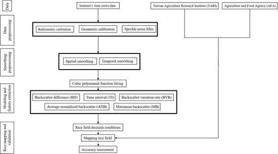
The Sentinel-1A data were pre-processed using the Sentinel Application Platform (SNAP) Sentinel-1 Toolbox software developed by ESA. Pretreatment includes three main steps. First, the radiometric calibration process was performed to convert the pixel data to actual backscattering values of sigma naught (dB). Thus, the pixel values in the imagery can be directly related to the radar backscatter of the scene. Then range Doppler terrain correction process corrected the geometric distortion in the range and projected range to Taiwan Datum 1997 (TWD97) earth ellipsoid model. Finally, the refined Lee filter [49] was applied to remove speckle noise in SAR data.

In this study, the proposed rice detection method is based on the rice-growth related features, which are extracted from the time-series backscatters during rice growth. Due to different farming behavior, such as different sowing dates, the heading or maturity dates of rice growth are also different. The times corresponding to minimum and maximum backscatter values are different for each rice-field. Therefore, instead of directly using backscatters, a model corresponding to backscattering change is established first, and then the rice features are extracted from the model.

However, the fluctuation of backscattering coefficients will cause model distortion and affect the extracted features, for example the maximum backscatter values and the growth time period. Therefore, it is difficult to model the rice growth curve effectively based on the acquired temporal data. 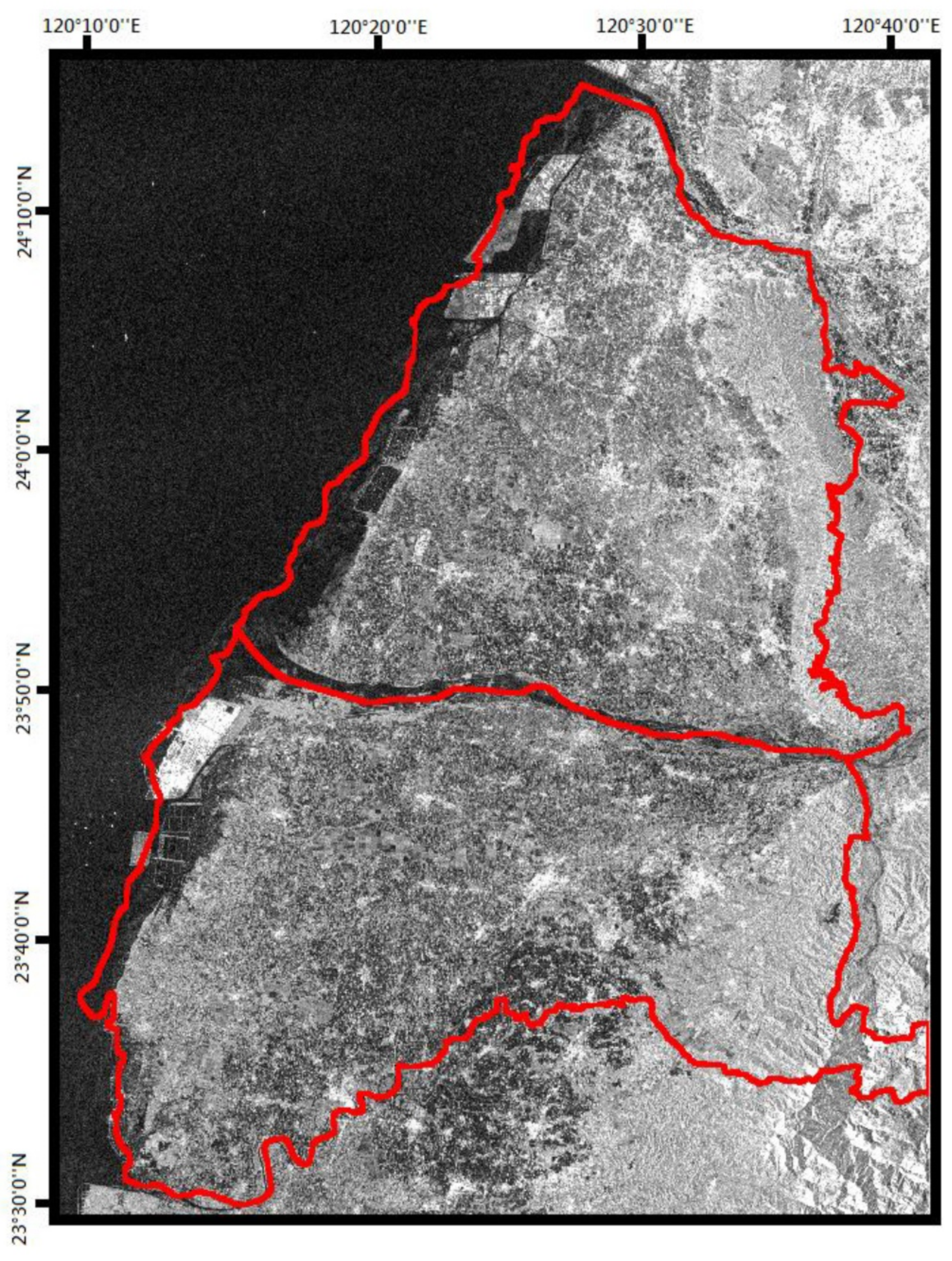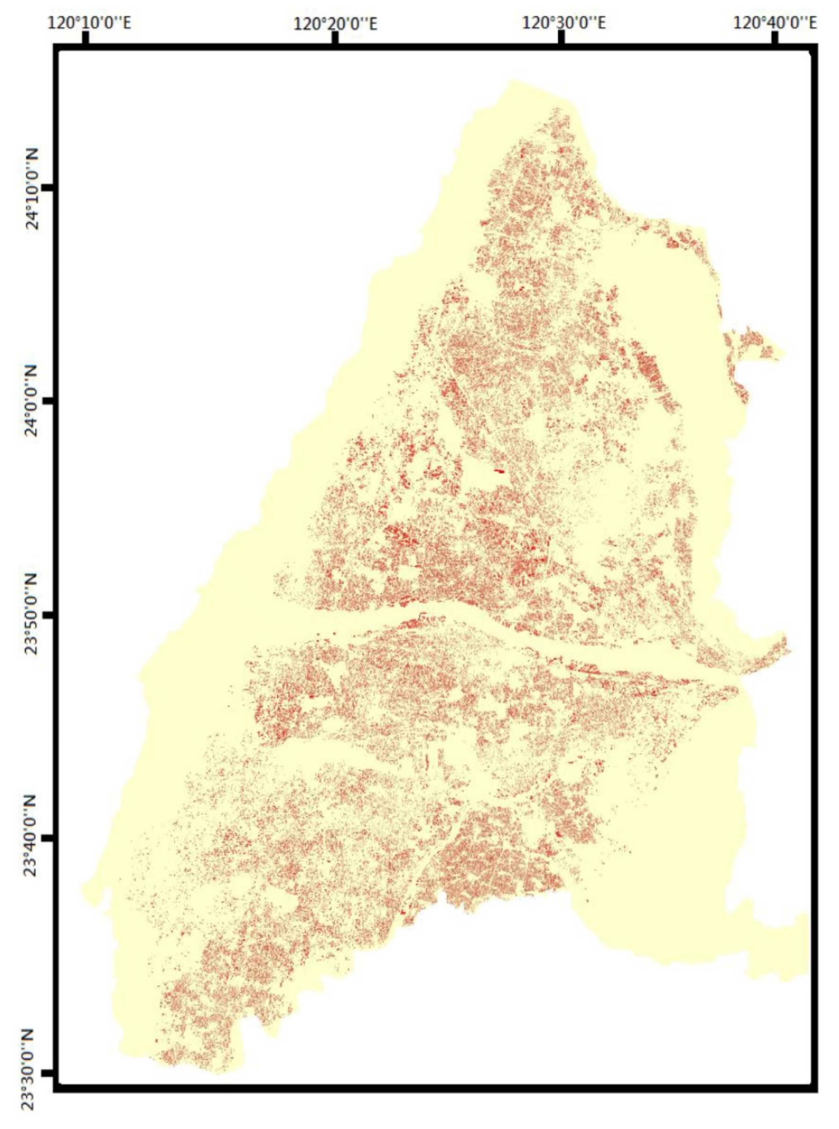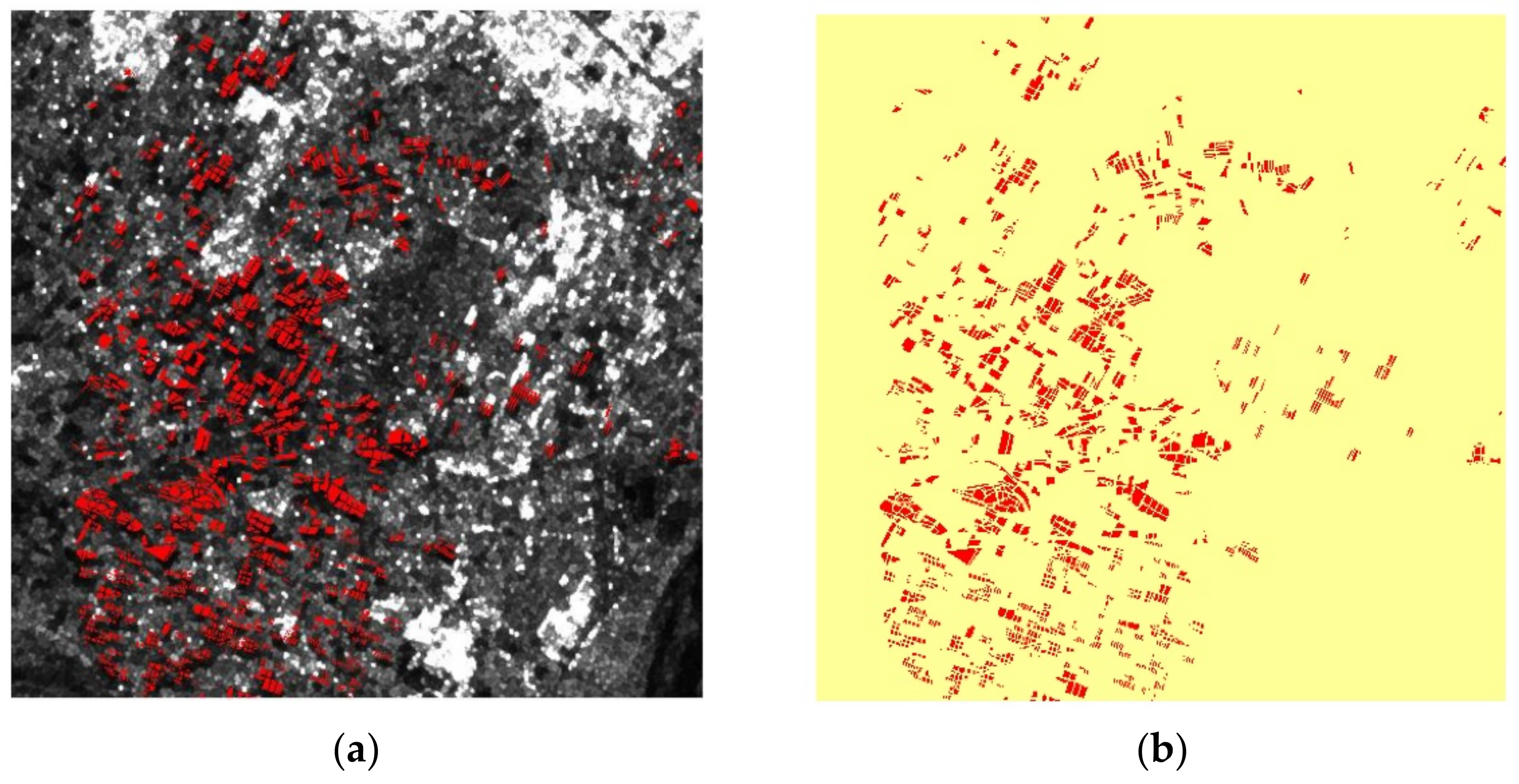To reduce the influence of the fluctuation of the backscattering coefficients, the SAR data are preprocessed by a smoothing approach [50]. Since the cultivation of crops was the block-based and clustered, a spatial mask was applied to perform pixel convolution for spatial smoothing. For example, the image in Figure 3a is the original SAR image in the study area. 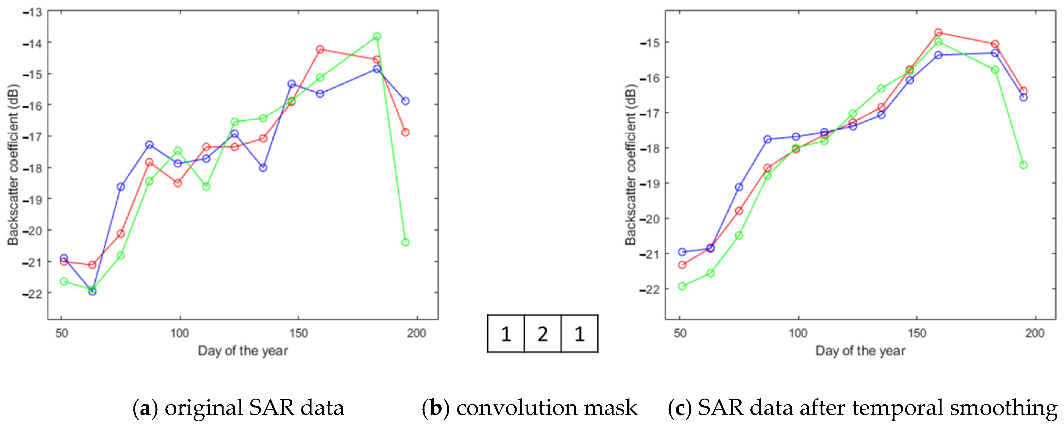After the spatial smoothing, the output image was smoother, as shown in Figure 3c. Subsequently, temporal smoothing is performed on each pixel by a convolution mask to alleviate the randomness of temporal evolution. As shown in Figure 4a, the original SAR data fluctuates greatly. The temporal backscatter coefficient is smoother and the randomness has been reduced after the temporal convolution.

2.4. Modeling and Feature Extraction

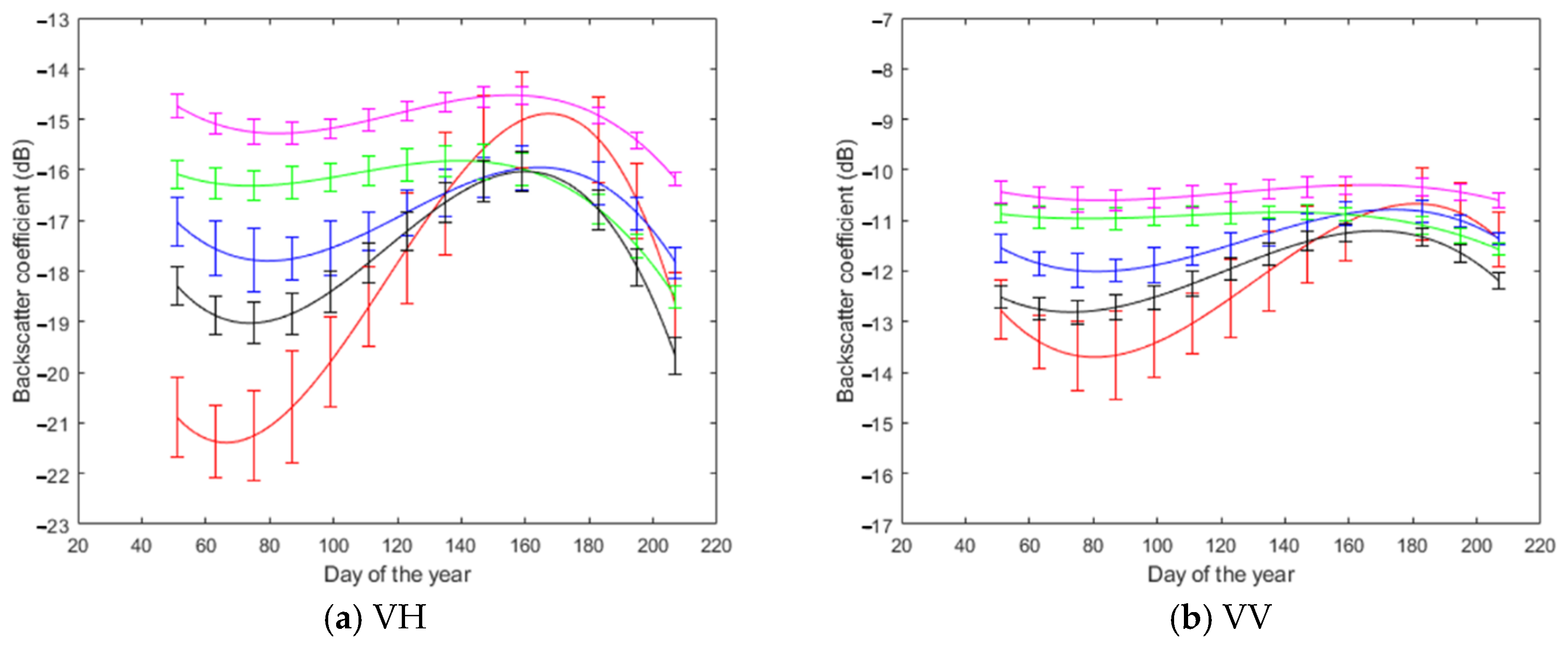
After smoothing processing, a model of rice growth curve was established based on the complete time-series data of the rice growth period. Observing the temporal data in Figure 4, the time corresponding to minimum and maximum backscattering values can represent the sowing and heading dates of rice growing, respectively. Therefore, the date corresponding to the minimum backscatter value of the time-series data can be used to locate the starting date of the rice growth period and complete time-series data were collected from this date.

Due to the different sowing dates, the length of the complete time-series data of each rice-field is different. To overcome this problem in the study, a cubic polynomial function was used to fit the collected time-series data, and a model of the rice growth trend curve was established. Figure 5 shows the fitting curves of rice and non-rice crops. In terms of electromagnetic interaction mechanisms between radar waves, vegetation canopy, soil and water, there was high correlation between paddy rice backscatter coefficient and its specific growth period [32,51,52]. In the sowing, agricultural land was underwater, so the backscatter from rice-field was dominated by the double bounce volume scattering. Therefore, the backscatter energy of water was greater than that of paddy rice. Water layers are smooth and homogenous, causing reflected radar pulses to be weak and the backscatter coefficient is low in the sowing of rice growth period. During the vegetative to heading perio, the backscatter coefficient showed a significant increase, due to the volume scattering from within the rice canopy and multiple reflections between the plants and water surface. The backscatter then decreases slightly during the reproductive to harvest period, due to the fact that the water content of the plant decreases, and so do stem and leaf densities [41,42,46]. In the study area, the non-rice food crops include corn, peanut, onion and wheat. Figure 5 shows the temporal variation of backscatter coefficient of rice and the above non-rice food crops under VH and VV polarizations. These backscatter variation curves were obtained by using 50 crop fields randomly selected from the ground truth data of each crop. In order to show the deviation between the backscattering curve and the real data, the curve in Figure 5 was represented by the mean value and the corresponding standard deviation bar for each food crop. Obviously, the backscattering coefficient of rice changes greatly during the growing period, while the backscattering changes of other crops (such as peanuts and onions) are smoother. Thus, the backscatter coefficient of paddy rice changes significantly during the rice growth period compared with other non-rice crops.

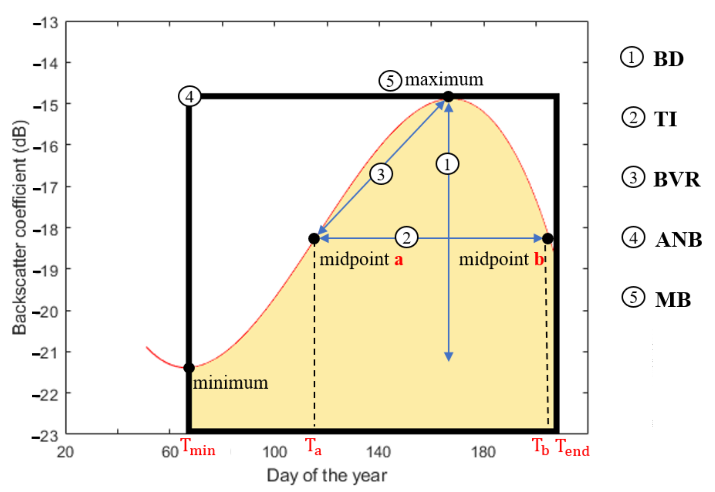
According to the growth and the cycle of rice crops, five features are extracted from the constructed rice growth trend model, as shown in Figure 5.

(1) Backscatter Difference (BD)

Compared with other non-rice crops in Figure 5, due to the obvious changes of rice plants during the growth period, the backscattering coefficient of rice also correspondingly changes significantly [30,33,34,36,37,38,40,41,42,43,44,46,47]. From the fitting curves of rice and non-rice in Figure 5, it can be observed that the backscatter change between the maximum and minimum values of rice is greater than that of other non-rice crops during the rice growing season (early Feb. to late Jul.). Thus, the backscatter difference (BD) between maximum and minimum values of time-series data during the rice growing season (from early Feb. to late Jul. in the study) was further examined for rice and non-rice crops, as shown in Figure 6. 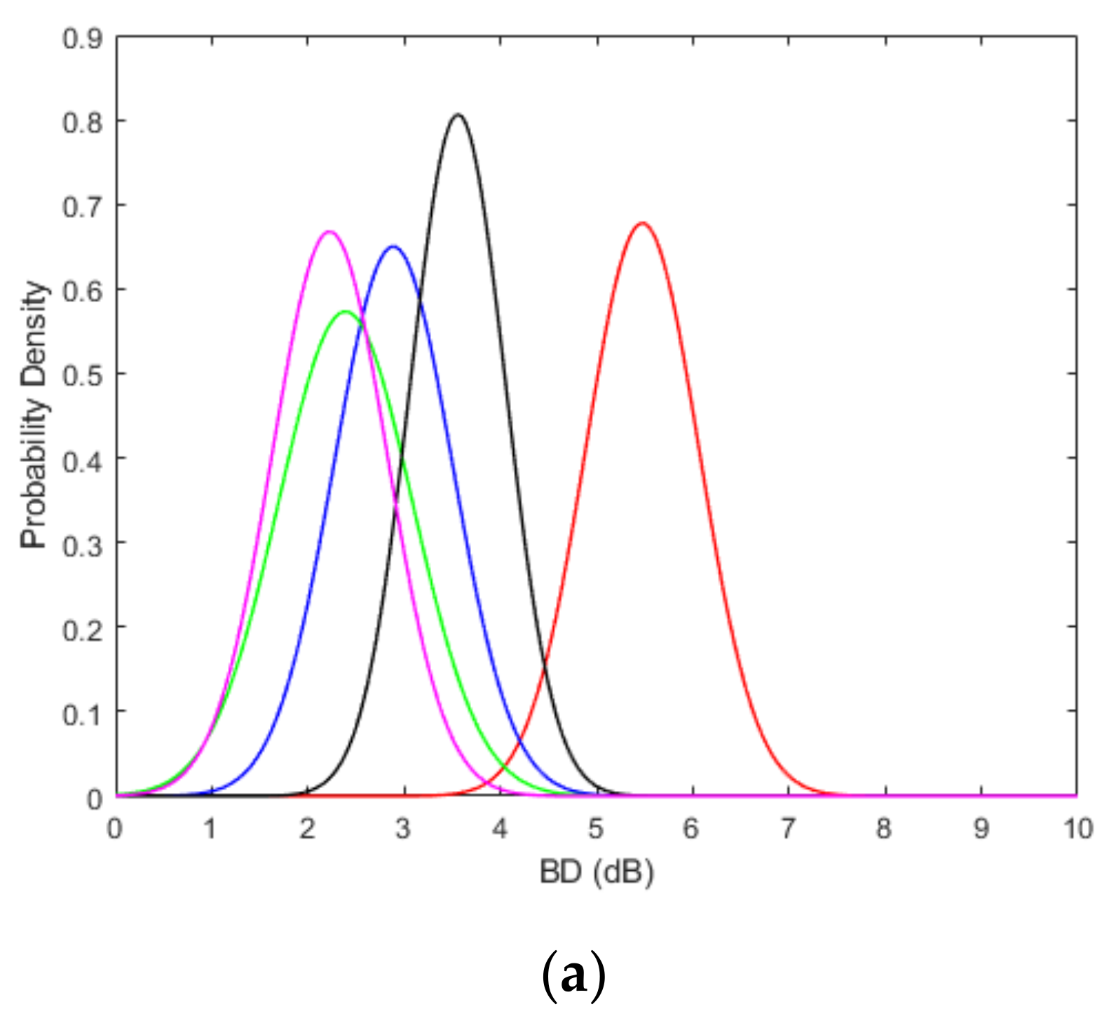Figure 7a shows the probability density functions (pdf) of BD for different crops. It can be observed that the BD values of rice are distributed in 4–7 dB, while the BD values of maize and wheat are distributed in 1–5 dB and 2–5 dB, respectively, and the others are distributed in 1–4 dB. These results indicate that BD can help distinguish rice from other non-rice crops in the study area. In this study, BD was selected as one feature in rice-field detection. In following rice detection, the BD threshold was set based on the 95% confidence interval of pdf from the training data (i.e., 4.3 dB ≤ BD ≤ 6.6 dB in experiments for VH polarization with ascending orbit mode).

(2) Time Interval (TI)

In addition to the characteristics of BD, the growth period of crops is also an important feature [31,33,36,37,40,41]. Each crop has its own specific growth time period. The growth cycle of rice is carried out in the order of sowing, vegetative growth, heading and maturity, which takes about four months in Taiwan. According to the rice growth model in Figure 6, the minimum backscatter point, the midpoint a, the maximum backscatter point and midpoint b are applied to represent the above four rice growth stages, respectively. The midpoints, a and b indicate the positions where the average value of the maximum and minimum backscatter appear in the rice growth curve. $T_a$ and $T_b$ are the corresponding dates of midpoint a and b, as shown in Figure 6. In the study, the time difference between two midpoints, $T_b-T_a$, of the rice growth curve, which denotes the time interval (TI) between vegetative growth and maturity, was used as one of the characteristics of rice growth. 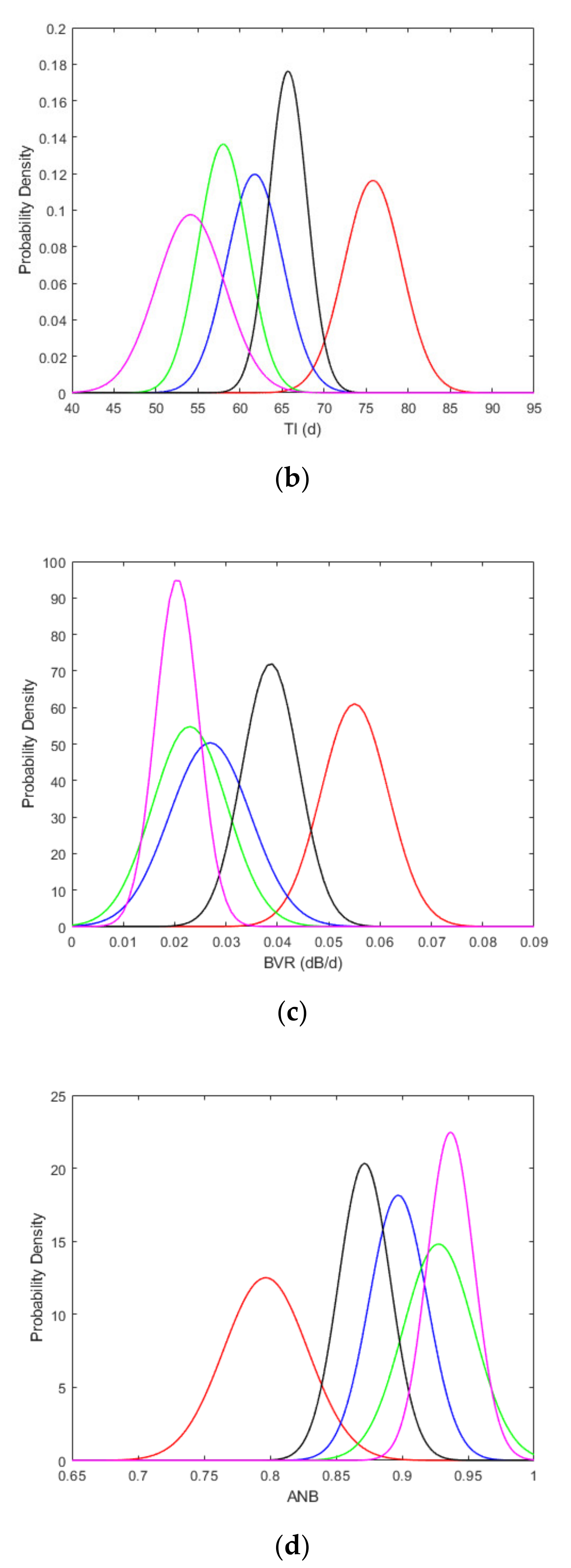The TI distributions of rice and non-rice crops are given in Figure 7b. It can be observed that the average TI of non-rice crops are 54, 58, 62 and 65 day for onion, peanut, maize and wheat, respectively, which are relatively smaller than the 76 day average TI of rice. In the experiment, the TI decision interval is between 69.0 day and 82.5 day based on the 95% confidence interval of TI distributions.

(3) Backscatter Variation Rate (BVR)

During the tillering, the variation rate of backscattering in rice is obviously accelerated. After the time corresponding to midpoint a of the curve in Figure 6, the backscatter of rice increases and reaches the peak at heading. Therefore, the slope from midpoint a to maximum backscatter point was used to represent the variation rate of backscattering at the tillering in the study, which is calculated by

$$\mathrm{BVR}=\frac{{\sigma }_{max}-{\sigma }_a}{T_{max}-T_a}$$

(1)

${\sigma }_{max}$ and ${\sigma }_a$ are the backscatter values at the maximum backscatter point and midpoint a, respectively. $T_{max}$ and $T_a$ represent the corresponding dates of maximum backscatter point and midpoint a, respectively. Figure 7c shows the pdfs of backscatter variation rate (BVR) for rice and non-rice crops. It can be observed that the BVR values of rice are larger than those of non-rice crops. According to the 95% confidence interval of the pdf, the values between $4.2\times {10}^{-2}$ dB/d and $6.7\times {10}^{-2}$ dB/d were chosen as the decision interval of BVR in the subsequent rice detection experiments.

(4) Average Normalized Backscatter (ANB)

The trend of rice growth formed by the backscatter coefficients is consistent with the rice growth cycle from sowing, heading to maturity. When the maximum backscatter value is normalized to one for each crop in Figure 5, it can be observed that the value of average normalized backscatter is close to one for a flatter curve, while this value becomes smaller for a curve with greater variation. The ANB is calculated by:

$$\mathrm{ANB}=\frac{1}{T_{end}-T_{min}} {{\displaystyle \int }}_{T_{min}}^{T_{end}}\frac{\sigma \left(t\right)}{{\sigma }_{max}} dt$$

(2)

$T_{min}$ and $T_{end}$ represent the corresponding dates of the minimum backscatter point and end point in the rice growth season, respectively. In the study, the average normalized backscatter (ANB) is the ratio of the integrated area of the normalized growth curve (with the maximum value normalized to 1) to the growth period, as shown in Figure 6. According to the pdfs of ANB shown in Figure 7d, the ANB of rice is much smaller than that of other crops. Therefore, ANB was also selected as an indicator of rice detection. The decision interval of ANB was chosen to be from $7.3\times {10}^{-1}$ to $8.6\times {10}^{-1}$ in the rice detection experiment.

(5) Maximum Backscatter (MB)

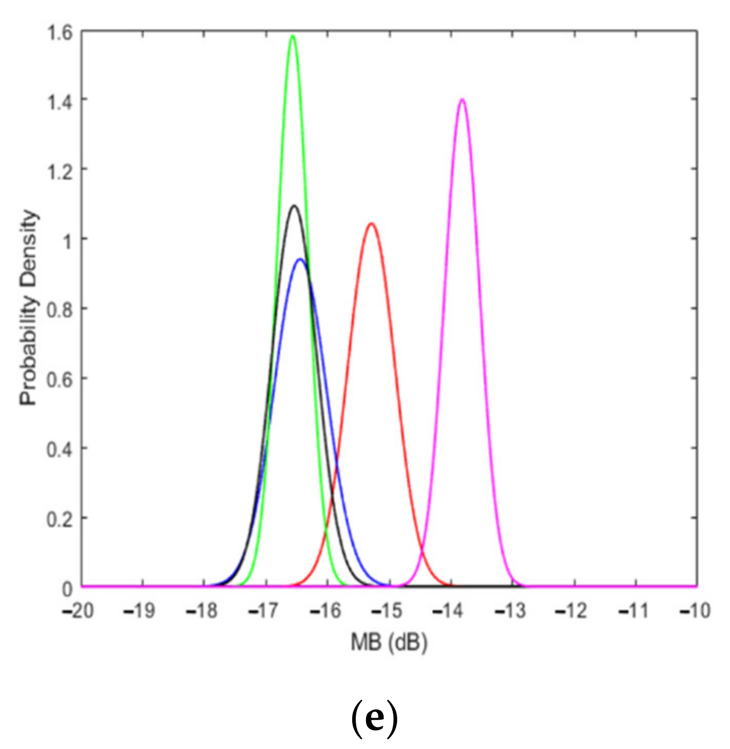
Each crop has its backscatter distribution range, and the corresponding maximum backscatter (MB) value is also different, as shown in Figure 5. The pdfs of the MB values are given in Figure 7e, which shows that the MB distribution of rice is different from other crops. In order to distinguish rice from other non-rice objects, MB is used as one of rice identification features in the study [33,36,37,40,45]. In the experiment, the decision interval of MB was chosen between −16.0 dB and −14.5 dB for rice detection.

The above five features can be extracted from the fitting models. Then the distribution of each feature is estimated from the training data of rice and non-rice, respectively. To detect rice crops, a feature-based decision method is introduced based on five extracted features. The decision threshold is determined by the 95% confidence interval of rice feature distribution, shown in Figure 7. Moreover, it can be observed from Figure 7 that the distributions of the extracted features of rice overlap with those corresponding to other non-rice crops. These reasons make rice detection difficult. If only one or two features are used for rice detection, some non-rice crops will be misclassified as rice. This leads to lower detection accuracy of non-rice. Therefore, this study proposed a decision method based on all five features, BD, TI, BVR, ANB and MB, to detect the mapping of rice-fields. When all five extracted features of the test field meet the decision conditions, this field is classified as rice, otherwise it is classified as non-rice. In experiments, the rice field is identified by the following decision rules:

$$\mathrm{Rice}\mathrm{field}\mathrm{conditions}:\left\{\begin{array}{c}4.3 \mathrm{dB}<BD<6.6 \mathrm{dB}\\ 69.0\mathrm{day}<TI<82.5\mathrm{day}\\ 4.2\times {10}^{-2}\mathrm{dB}/\mathrm{day}<BVR<6.7\times {10}^{-2}\mathrm{dB}/\mathrm{day}\\ 7.3\times {10}^{-1}<ANB<8.6\times {10}^{-1}\\ -16.0\mathrm{dB}<MB<-14.5\mathrm{dB}\end{array}\right.$$

(3)

2.5. Classification Algorithms

To evaluate the performance of the proposed method, the detection results were compared with four other classification algorithms: decision tree (DT) [53], support vector machine (SVM) [54], K-nearest neighbor (KNN) [55] and quadratic discriminant analysis (QDA) [56]. DT, SVM and KNN are non-parametric supervised learning methods for classification. The DT classifier infers the decision rules from data features and divides the input dataset into categorical classes by recursive partitioning based on the splitting rules. SVM classifier constructs a hyperplane, through which a good separation can be achieved. That is the constructed hyperplane has the largest distance to the nearest training-data point of any class. The KNN classifier predicts the target label by finding the nearest neighbor category which is determined based on the distance measures. QDA is a statistical classifier that uses a quadratic decision surface to separate measurements of two or more classes. The decision boundary is generated by fitting class conditional densities to the data based on Bayes’ rule.

Moreover, for DT, SVM and KNN classifiers, there are three scales to be considered in the experiment, namely Fine, Medium and Coarse, provided by MATLAB Machine Learning Toolbox. Rice detection performance was verified by 5-fold cross-validation [57] in MATLAB. The 5-fold cross-validation splits the dataset into five equal parts. In experiments, four parts were used as training data, and the remaining parts were used as test data. This process was repeated five times and the results averaged, each time using one different part as the testing data.

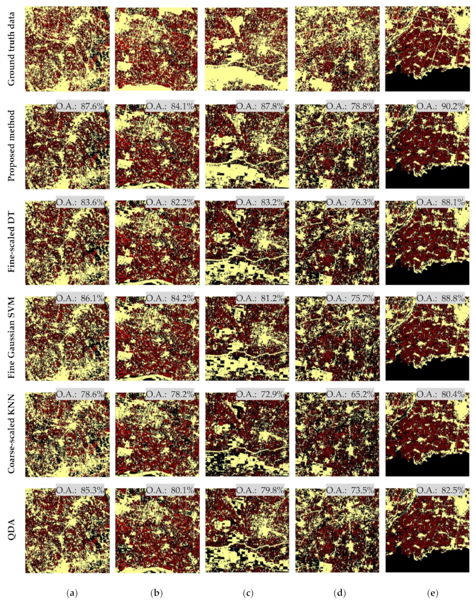
In the rice-field mapping experiment in Section 3.3, all image pixels will be used instead of only the samples of the dataset. Due to the clustering characteristics of crop planting, the image was first partitioned into clusters by the fuzzy c-means algorithm [58]. Therefore, pixels with similar temporal characteristics were grouped into a cluster. The corresponding model and rice-growth features of each cluster will be utilized in the subsequent rice detection.

3. Results

In this section, experiments were performed to verify the efficiency of the proposed rice-field detection method. Yunlin and Changhua counties, the most important rice growing areas in Taiwan, were selected as the study areas. The topographical characteristics of rice growing areas in these two counties are similar. There are no crops in the east, because these areas are the highlands and hills of the two counties. The coastal area is not suitable for rice growth due to the northeast monsoon. The planting area near the coast is scattered and small, and some short-term crops such as peanuts and garlic are grown. Compared with the eastern and coastal areas, the rice planting area is more extensive and denser in the inland areas of these two counties. In experiments, we have selected five regions from the inland area of Yunlin and Changhua counties and the image size of each region is 1000 × 1000 pixels, as shown in Figure 8 and Figure 9. Regions 1 and 2 are both located in the Changhua County. Regions 3 and 4 are in Yunlin County. Region 5 is located in Yunlin County, except for the bottom.

For region 1, the farmland in this area is mainly for growing rice, but the rice-fields are scattered. Most of the non-rice areas are covered by buildings sparsely distributed in farmland.

In region 2, the agricultural land is intensive and rice is the main crop. According to the ground data of TARI, a few of the croplands are covered by peanut, garlic and watermelon. Similar to region 1, most of the buildings are scattered in this area.

Region 3 is the main agricultural land in Yunlin. Most farmland grows rice, but other non-rice fields, such as peanut, garlic, maize and cabbage, are scattered in this region.

There are diverse crops in the area of region 4. The crops contain rice, peanut, garlic, cabbage, potato and edamame. Although rice is the main crop in region 4, the rice-fields in this region are scattered and relatively small (less than 0.5 ha) compared with the average area of rice fields in other regions, about 0.5 ha.

In region 5, agricultural land is densely distributed and only rice is grown. Some buildings are sparsely located in this area. Besides, the bottom of region 5 is outside of the Yunlin County and there is no ground truth data for rice mapping, so it is marked as a non-interesting area shown in black in Figure 9e.

In the experiment, a dataset consisting of rice and non-rice samples was prepared. According to the ground truth data, 10,000 polygon fields of rice and non-rice were randomly selected from the above five regions, separately. There are a total of 50,000 rice and non-rice polygon fields, respectively. To evaluate the efficiency of the proposed method, the dataset was divided into training and testing samples in which 80 percent of samples (40,000 rice fields and non-paddy fields, respectively) were regarded as training data and 20 percent of samples (10,000 rice fields and non-paddy fields, respectively) were regarded as testing data. In the following, the features of rice were first extracted from the training data and approximated by using Gaussian distributions. Then, the decision criterion of each feature was determined according to the 95% confidence intervals of the corresponding feature distribution. Finally, the test data was used to evaluate the detection accuracy for the proposed feature-based rice decision method.

3.1. Accuracy Assessment

In this experiment, we compared the rice detection performance of the extracted rice growth features, including backscatter difference (BD), time interval (TI), backscatter variation rate (BVR), and average normalized backscatter (ANB). In addition, the simulation scenario contains two polarizations (VH and VV) and two orbit modes (ascending and descending).

First, rice detection experiments were conducted using only one extracted feature at a time. The maximum backscatter (MB) feature was not included in the simulation, because MB is suitable for use with other features.

Table 3. Detection accuracy of the proposed features for VH polarization with ascending orbit mode. The P.A., U.A. and O.A. represent the producer accuracy, user accuracy and overall accuracy, respectively.

	Features	Rice		Non-Rice		O.A. (%)
		P.A. (%)	U.A. (%)	P.A. (%)	U.A. (%)
One feature	BD	91.1	82.4	80.6	90.0	85.8
	TI	92.3	85.7	84.6	91.6	88.4
	BVR	90.8	83.0	81.5	89.8	86.1
	ANB	90.3	82.5	80.9	89.2	85.6
Combined features	BD + TI	91.9	89.7	89.5	91.7	90.7
	BD + TI + BVR	91.5	91.2	91.2	91.4	91.3
	BD + TI + BVR + ANB	91.3	91.7	91.8	91.3	91.5
	All	90.9	92.1	92.3	91.0	91.6

shows the detection results under the experimental situation of VH polarization and ascending orbit mode. The classification overall accuracy (O.A.), user accuracy (U.A.) and producer accuracy (P.A.) were calculated from the confusion matrix [59]. It can be observed that the P.A. and O.A. of rice achieve over 90% and 85%, respectively, for each feature. These results validate the efficiency of the extracted features in rice detection. Moreover, the detection efficiency of feature TI is superior to other features. The effectiveness of TI in rice identification is due to the rice growing period being about 120 days, which is significantly different from other crops in this area. For example, the growing period of garlic is about 90 days in Yunlin County.

The results in Table 3 also show that the accuracy of non-rice detection is much lower than that of rice detection. To improve the performance of non-rice detection, we performed the rice detection next by using the combined features. Five experiments were conducted here, including one feature (BD), two features combined (BD and TI), three features combined (BD, TI and BVR), four features combined (BD, TI, BVR and ANB) and all five features combined. Table 3 shows that the simulation scheme with two combined features can improve O.A. by about 5% compared with the case of using only one feature. Regarding the case with three or more features, the O.A. of rice slightly increases by about 1% and the P.A. of non-rice crops increases by about 2–3%, compared with the case using two features. With the increase in the number of combined features, the O.A. of rice and the P.A. of non-rice crop detection are still improved. Compared with only using feature BD, the P.A. of non-rice crops can be improved by about 12% by the combined use of all combined features, although the P.A. of rice crops is slightly reduced, it still remains above 90%. In general, the proposed method with combined features can achieve more than 90% O.A. in rice detection. These experimental results validate the efficiency of the proposed method based on the combined rice growth features.

Then, we examined the influence of polarizations and orbital modes on rice detection.

Table 4. Detection accuracy of all combined features for different orbit modes and polarizations.

Orbit Modes	Polarizations	Rice		Non-Rice		O.A. (%)
		P.A. (%)	U.A. (%)	P.A. (%)	U.A. (%)
Ascending	VH	90.9	92.1	92.3	91.0	91.6
	VV	82.1	85.7	86.3	82.8	84.2
Descending	VH	90.4	92.0	92.2	90.5	91.3
	VV	84.0	88.3	88.9	84.7	86.4

shows the results of the proposed method with all combined features for VH and VV polarizations with ascending and descending orbit modes. The O.A. is 91.6% and 91.3% for VH polarization with ascending and descending orbit modes, respectively. The orbit mode does not significantly affect the detection results. This result may come from the fact that incidence angles for the ascending and descending orbital modes are very close in the study area, which are from 31.5 to 36.3° and 31.8 to 36°, respectively. However, the O.A. is 84.2% and 86.4% for VV polarization with ascending and descending orbit modes, respectively. Thus, the rice detection accuracy of VH polarization is much better than that of VV polarization. This result is the same as the studies [33,43,51]. Compared with VV, VH is more representative of the actual rice growth structure and can provide more information in paddy rice distinguishing. Based on the above results, the simulation scheme of VH polarization with ascending orbit mode will be considered in the following experiments.

Next, an experiment was conducted to compare the accuracy of rice detection with and without smoothing preprocessing. In addition, most studies in the literature use the maximum and minimum backscatter coefficients to detect rice fields. Therefore, they can apply the raw backscatter coefficient data without smoothing. In the experiment, we compared the performance of all five features (with and without smoothing). As shown in

Table 5. Detection accuracy of the combined features with and without smoothing processing for VH polarization with ascending orbit mode.

Features	Smoothing Processing	Rice		Non-Rice		O.A. (%)
		P.A. (%)	U.A. (%)	P.A. (%)	U.A. (%)
All	Yes	87.5	83.2	91.5	93.7	90.2
All	No	67.3	70.4	86.4	84.5	80.1

, the O.A. of the proposed method using all five features is 90.2% and 80.1% with and without smoothing, respectively. The reason for the lower O.A. of the proposed method without smoothing processing is that the P.A. of rice is only 67.3%. This is due to model distortion caused by fluctuations in the backscattering coefficient and certain features such as TI and BVR are highly dependent on built models. Thus, the smoothing processing is important to establish the backscatter variation model for the proposed method.

3.2. Classifier Comparison

In the experiment, the rice detection performance of the proposed method was compared with four other classification algorithms: DT, SVM, KNN and QDA, by using the dataset as in Section 3.1. The dataset consists of the rice and non-rice samples from five regions in Figure 9. Rice detection performance was verified by 5-fold validation in MATLAB and O.A., U.A. and P.A. were evaluated by using 100 Monte Carlo trials for all classifiers. The experiments were conducted using all extracted features as input data for all classification algorithms. In addition, three scales, Fine, Medium and Coarse, were considered for DT, SVM and KNN classifiers, provided by MATLAB Machine Learning Toolbox.

Table 6. Comparison of the proposed method with the other four classifiers for VH polarization with ascending orbit mode, including O.A., U.A., P.A. and kappa.

Classifiers		Rice		Non-Rice		O.A. (%)	Kappa
		P.A. (%)	U.A. (%)	P.A. (%)	U.A. (%)
Proposed Method		91.2	92.4	92.6	91.3	91.9	0.83
DT	Fine	85.3	87.2	87.5	85.6	86.4	0.72
	Medium	82.2	85.7	86.4	82.9	84.3	0.68
	Coarse	88.1	73.2	67.7	85.0	77.9	0.55
Gaussian SVM	Fine	88.3	88.9	88.9	88.3	88.6	0.77
	Medium	82.3	85.7	86.4	83.0	84.3	0.68
	Coarse	85.3	77.4	75.1	83.6	80.2	0.6
KNN	Fine	96.9	62.3	41.5	93.0	69.2	0.38
	Medium	92.6	68.5	57.4	88.5	75.0	0.50
	Coarse	86.5	77.0	74.1	84.5	80.3	0.60
QDA		85.7	77.6	75.3	84.0	80.5	0.61

summarizes the detection results of all classifiers. SVM classifiers are one of the favorite methods in remote sensing research. In fact, they provide better performance than the other three classifiers, in addition to the proposed method. Among all SVM classifiers, the best one is SVM with a fine Gaussian kernel. The overall classification accuracy and kappa coefficient are 88.6% and 0.77, respectively. In addition, the fine-scaled KNN classifier achieves a high rice P.A. of 96.9%, but O.A. is only 69.2% which is due to the poor non-rice detection ability of KNN. Among the three scaled KNN classifiers, only coarse-scaled KNN has better classification performance, with 80.3% O.A. and 0.6 kappa. Compared with the other four classifiers, the proposed method can achieve higher classification accuracy with 91.9% O.A. and 0.83 kappa.

3.3. Mapping Rice-Field Distribution

In this experiment, rice-field mapping of the study area was detected by the pre-trained classifiers in Section 3.2. According to the results of Table 6, the best scale of DT, SVM and KNN was selected for the rice detection. Thus, five classifiers were considered in the experiment, including the proposed method, fine-scaled DT, SVM with fine Gaussian kernel, coarse-scaled KNN and QDA. Instead of samples of the dataset, all image pixels were exploited in the experiment.

The rice detection results of the five selected regions are given in Figure 10 and

Table 7. Detection accuracy of the five regions by the proposed method and the other four classifiers for VH polarization with ascending orbit mode.

Regions	Classifiers	Rice P.A. (%)	Non-Rice P.A. (%)	O.A. (%)
1	Proposed method	84.7	88.4	87.6
	Fine-scaled DT	86.7	82.7	83.6
	Fine Gaussian SVM	80.3	87.4	86.1
	Coarse-scaled KNN	70.4	80.9	78.6
	QDA	84.2	85.6	85.3
2	Proposed method	82.4	84.8	84.1
	Fine-scaled DT	81.2	82.6	82.2
	Fine Gaussian SVM	82.3	85.0	84.2
	Coarse-scaled KNN	85.1	75.2	78.2
	QDA	88.4	76.5	80.1
3	Proposed method	83.8	88.7	87.8
	Fine-scaled DT	83.6	83.1	83.2
	Fine Gaussian SVM	88.3	79.5	81.2
	Coarse-scaled KNN	91.5	68.4	72.9
	QDA	87.5	77.9	79.8
4	Proposed method	90.1	76.1	78.8
	Fine-scaled DT	88.0	73.5	76.3
	Fine Gaussian SVM	91.4	72.0	75.7
	Coarse-scaled KNN	89.6	59.4	65.2
	QDA	87.7	70.1	73.5
5	Proposed method	87.5	91.5	90.2
	Fine-scaled DT	86.8	88.8	88.1
	Fine Gaussian SVM	87.5	89.4	88.8
	Coarse-scaled KNN	90.0	75.7	80.4
	QDA	92.3	77.7	82.5

. Figure 10 shows the rice-field mapping in which rice and non-rice pixels are shown in red and yellow, respectively, and non-interesting area in black. The detection accuracy of all classifiers was summarized in Table 7. Due to the large disparity in the number of pixels between rice fields and non-rice fields in the selected regions, the detection accuracy was determined by P.A. and O.A. in Table 7. Comparing the detection results of the five selected regions with the ground truth data in Figure 10, it can be observed that most rice fields can be correctly detected by the classifiers. As shown in Table 7, the rice P.A. of five selected regions can achieve over 80% for all classifiers. One exception is the poor rice detection performance of the KNN classifier in region 1. In region 2, the performance of the proposed method is similar to SVM, with 84.1% and 84.2% O.A., respectively. Obviously, the proposed method provides a non-rice P.A. of 88.7%, higher than the other classifiers in region 3. Whereas in region 4, the O.A. of all classifiers are lower than 80%, due to the poor detection efficiency of non-rice. Almost all classifiers can provide effective rice detection in region 5, especially the proposed method which can reach a high O.A. of 90.2%. Compared with other regions, the cultivated lands in region 4 are relatively small (less than 0.5 ha), densely distributed and have more non-rice species planted. Therefore, the backscattering of rice is affected by nearby non-rice crops. However, in this experiment, the decision criterion was determined based on the 95% confidence interval from the feature distributions of all training data. The decision parameters were not adjusted for the case of more diverse crop species. Thus, non-rice detection accuracy in region 4 is lower than other regions, resulting in lower overall detection accuracy. In contrast, rice fields are densely distributed and the crop types are single in region 5, so overall detection accuracy is better than other regions. Therefore, the diversity of crops and the dispersion degree of farmlands may affect the detection results. However, in all experimental regions, the proposed method can consistently provide higher classification accuracy than the other four classifiers.

In addition, to evaluate the efficiency of the proposed method, the processing timing of rice detection was evaluated by using selected region 5 with image size 1000 × 1000 pixels. The execution time of proposed method is 0.6 s. As for other classifiers, SVM takes more than 20 s, DT takes about 1.5 s, QDA takes about 1.2 s and KNN classifier takes about 2 s.

In the following experiment, we further estimated the rice-fields of Yunlin and Changhua counties by the proposed method. The rice field mapping of the study area is shown in Figure 11 with rice pixels colored in red. In order to clearly present the predicted results of rice-fields, three regions selected from Figure 11 were compared with the corresponding ground truth in Figure 12. Most of rice-fields can be detected by the proposed method except for a few sporadic agricultural lands (shown in the black circles in Figure 12). Obviously, the farmlands in these areas are small and scattered. The detection errors may be caused by other planting of crops, such as peanuts and garlic, between rice fields. According to the statistical data from AFA in 2017 (http://210.69.71.166/Pxweb2007/Dialog/statfile9L.asp), the total area of rice-field cultivation is 58,829.6 ha in Yunlin and Changhua counties. By using the proposed method, the total rice-field area in the study counties was estimated to be 54,673.79 ha based on the results in Figure 11, and the rice detection accuracy reached 92.9%.

4. Discussion

Rice growth has a specific time sequence, from transplanting, heading to maturity. The variation of rice plants at different growth stages is reflected in the SAR backscatter value. The study has made full use of the phenological characteristics of rice, and proposed the associated features of rice growth based on the temporal SAR backscatter values. All extracted features were combined for rice detection. Experiment results validate the efficiency of the proposed rice-field detection, with OA greater than 90%.

Other researches [38,60] have also detected the distribution of rice fields in the same study area as ours. Jyun-bin [38] utilized the Normalized Difference Sigma-naught Index (NDSI), which is calculated based on the maximum and minimum backscatter values of the Sentinel-1A time-series data. NDSI is the same as the proposed feature BD, which achieves 85.8% overall detection accuracy as shown in Table 3. Chia-Hao [60] proposed a temporal-local binary pattern (T-LBP) method which combined time-series SAR data and local binary patterns. T-LBP describes the temporal change pattern of rice pixel in time-series Sentinel-1 image by applying LBP operator into temporal SAR backscatter. The results of [60] showed that the overall accuracy, rice-fields’ user accuracy and rice-fields’ producer accuracy were 74.1%, 72.2% and 77.6%, respectively.

To demonstrate the flexibility of the proposed method with different training and testing data, an experiment was conducted based on the same dataset as in Section 3.1, but using the samples in one region as training data, and the remaining samples in other regions as test data. For example, the decision model was pre-trained by using the samples from region 1 and tested by the data in regions 2–5. Therefore, in the experiment, there are 20% training data (10,000 rice fields and non-paddy fields) and 80% test data (40,000 rice fields and non-paddy fields). The detection results for VH polarization with ascending orbit mode in 2017 were summarized in

Table 8. The overall accuracy for different training and testing data for VH polarization with ascending orbit mode in 2017.

	Test	Region 1	Region 2	Region 3	Region 4	Region 5	Average O.A.
Train
Region 1		N/A	92.3	91.6	90.4	89.8	91.0
Region 2		91.9	N/A	91.2	91.1	89.6	91.0
Region 3		89.7	90.3	N/A	91.0	88.9	90.0
Region 4		89.6	90.1	89.8	N/A	88.4	89.5
Region 5		92.1	91.9	91.8	91.4	N/A	91.8

N/A: not applicable.

. The results show that the pre-trained model based on the data in region 5 has a better testing average O.A. than the models based on other regions, where the average O.A. is the average value of O.A. of the other four testing region. Whereas, the pre-trained model based on region 4 has a lowest average O.A. These results may come from the difference in the complexity of crops. As mentioned in Section 3.1, there are multiple crops planted in region 4 and a single rice crop grown in region 5. In addition, the mean of average O.A. from different training regions is 90.7% which was 1% lower than the O.A. in Table 3. The results verify the effectiveness of the proposed method under different training data.

Furthermore, in order to validate the stability of the proposed method in different years, the pre-trained classifier in Section 3.2 was applied to estimate the rice-fields of five selected regions, shown in Figure 8, in 2018. The detection results in 2017 and 2018 were summarized in

Table 9. Detection accuracy in 2017 and 2018 by the proposed method for VH polarization with ascending orbit mode.

Regions	Years	Rice		Non-Rice		O.A. (%)
		P.A. (%)	U.A. (%)	P.A. (%)	U.A. (%)
1	2017	84.7	67.5	88.4	95.3	87.6
	2018	83.8	68.0	88.8	95.0	87.7
2	2017	82.4	70.3	84.8	91.7	84.1
	2018	80.7	67.6	83.1	90.8	82.4
3	2017	83.8	63.9	88.7	95.8	87.8
	2018	83.6	64.3	88.9	95.8	87.9
4	2017	90.1	46.9	76.1	97.0	78.8
	2018	89.8	45.0	74.2	96.8	77.1
5	2017	87.5	83.2	91.5	93.7	90.2
	2018	86.7	81.3	90.4	93.3	89.2

. As shown in Table 9, rice P.A. of the five selected regions in 2018 were slightly lower than the detection results in 2017. For regions 2, 4 and 5, the O.A. values in 2018 were slightly lower than those in 2017, while for regions 1 and 3, the O.A. values in 2018 were slightly higher than those in 2017. Thus, by using the pre-trained classifier in 2017, the accuracy of rice detection can be maintained in 2018 for all selected regions.

Then, the performance of the pre-trained classifier in Section 3.2 was further tested by using one experimental area in Hualien County, which is located in eastern Taiwan. The mountainous terrain of Hualien County is very different from the topographic features of Yunlin and Changhua counties. The selected experimental area was shown in Figure 13 with an image size of 500 × 500 pixels. The P.A. of rice and non-rice is 91.7% and 83.8%, respectively. The O.A. is 84.3% in Hualien County. These results validate the stable performance of the proposed method in different terrain areas.

Instead of using the SAR backscattering coefficients directly, the proposed method uses the SAR temporal variation of rice plots during rice growing season to extract rice features. Therefore, the proposed combined-feature method can accurately detect rice fields in different years and regions. In future research, combinations of different polarizations will be considered for rice-field detection. The combination of VH and VV polarizations should provide more features of rice, thereby improving the performance of the proposed method in rice detection.

5. Conclusions

In the study, a rice detection method based on the rice growth-related features was proposed by using the Sentinel-1A time-series SAR data. Five rice growth related features were introduced, including BD, TI, BVR, ANB and MB.

Experiments conducted using only one feature show that the detection accuracy of feature TI, with 88.4% O.A., is higher than other features, as shown in Table 3. In the study, the feature-based rice decision method with the combination of all five features was proposed. This method can achieve over 90% overall detection accuracy through test dataset verification. In addition, experiments have examined the effectiveness of the proposed method in paddy field mapping. The results show that the proposed method can reach the rice detection accuracy of 91.9% O.A. and 0.83 kappa. Compared with the best classifiers among the other four classifiers (DT, SVM, KNN and QDA), the detection accuracy O.A. of the proposed method was 3% higher than that of the fine SVM classifier, as shown in Table 6. Furthermore, the proposed method has been verified to have consistently high rice detection accuracy in different years and regions. In conclusion, the proposed method can improve the accuracy of rice detection and is effective in rice-field mapping for the experimental areas of Yunlin County and Changhua County in central Taiwan.