Article

Variable Urbanization Warming Effects across Metropolitans of China and Relevant Driving Factors

1
Key Laboratory of Environmental Change and Natural Disaster, Ministry of Education, Beijing Normal University, Beijing 100875, China
2
Faculty of Geographical Science, Academy of Disaster Reduction and Emergency Management, Beijing Normal University, Beijing 100875, China
3
State Key Laboratory of Earth Surface Processes and Resource Ecology, Beijing Normal University, Beijing 100875, China
*
Author to whom correspondence should be addressed.
Remote Sens. 2020, 12(9), 1500; https://doi.org/10.3390/rs12091500
Submission received: 5 April 2020 / Revised: 28 April 2020 / Accepted: 30 April 2020 / Published: 8 May 2020
(This article belongs to the Section Environmental Remote Sensing)

Abstract

:
Urbanization is mainly characterized by the expansion of impervious surface (IS) and hence modifies hydrothermal properties of the urbanized areas. This process results in rising land surface temperature (LST) of the urbanized regions, i.e., urban heat island (UHI). Previous studies mainly focused on relations between LST and IS over individual city. However, because of the spatial heterogeneity of UHI from individual cities to urban agglomerations and the influence of relevant differences in climate background across urban agglomerations, the spatial-temporal scale independence of the IS-LST relationship still needs further investigation. In this case, based on Landsat-8 Operational Land Imager and Thermal Infrared Sensor (Landsat 8 OLI/TIRS) remote sensing image and multi-source remote sensing data, we extracted IS using VrNIR-BI (Visible red and NIR-based built-up Index) and calculated IS density across three major urban agglomerations across eastern China, i.e., the Beijing-Tianjin-Hebei (BTH), the Yangtze River Delta (YRD), and the Pearl River Delta (PRD) to investigate the IS-LST relations on different spatial and temporal scales and clarify the driving factors of LST. We find varying warming effects of IS on LST in diurnal and seasonal sense at different time scales. Specifically, the IS has stronger impacts on increase of LST during daytime than during nighttime and stronger impacts on increase of LST during summer than during winter. On different spatial scales, more significant enhancing effects of IS on LST can be observed across individual city than urban agglomerations. The Pearson correlation coefficient (r) between IS and LST at the individual urbanized region can be as high as 0.94, indicating that IS can well reflect LST changes within individual urbanized region. However, relationships between IS and LST indicate nonlinear effects of IS on LST. Because of differences in spatial scales, latitudes, and local climates, we depicted piecewise linear relations between IS and LST across BTH when the IS density was above 10% to 17%. Meanwhile, linear relations still stand between IS density and LST across YRD and PRD. Besides, the differences in the IS-LST relations across urban agglomeration indicate more significant enhancing effects of IS on LST across PRD than YRD and BTH. These findings help to enhance human understanding of the warming effects of urbanization or UHI at different spatial and temporal scales and is of scientific and practical merits for scientific urban planning.

Graphical Abstract

1. Introduction

Urbanization refers to a series of economic and social changes caused by the population gathering toward cities, which leads to the expansion of city size [1]. In recent decades, the development of urbanization has accelerated remarkably [2]. Booming urbanization results in the widespread conversion of farmlands, wetlands, or lakes into urban areas [1], which causes notable perturbations to the earth’s surface energy balance [3] and resultant increase in sensible heat flux at the expense of latent heat flux [4,5]. This has resulted in the phenomenon that land surface temperature (LST) is higher in urban areas than in the surrounding rural areas, pointing to one of the most important human impacts on the local surface climate, which is known as the Urban Heat Island (UHI) [3,6,7]. Nowadays urban areas are home to more than half of the global population, and this proportion will reach 60% by 2030 [8,9]. Meanwhile, negative effects of UHI on ecosystem, human society and human health in particular have been widely recognized such as alterations of biodiversity [10], modification of precipitation patterns [9], increased morbidity and mortality, and increased risk of violence as well [11,12] intensified extreme urban heat under future heat [13]. Therefore, UHI has been arousing growing human concerns in recent decades [1,5,6,7].
UHI can be subdivided into two types according to different temperature variables [14], i.e., the surface UHI measured by the LST [15] and the atmospheric UHI measured by the air surface temperature [16]. Air surface temperatures are affected by land cover changes, anthropogenic heat emissions, and air convection [17,18]. Compared to atmospheric UHI, the reasons for surface UHI changes include changes in the land surface properties caused by land cover and land use changes, anthropogenic heat emissions, etc. This current study focuses mainly on the UHI effects that are closely related to urban land cover types and land surface temperature. Currently, remote sensing technology plays an important role in the study of UHI, especially thermal remote sensing [19,20,21]. It can help to effectively investigate and understand the surface thermal condition, comprehensively research the formation and distribution characteristics of UHI [22]. Remote sensing monitor technology has the advantages of wide range, continuous observation for a long time, and is not affected by climate condition. With the development of high-resolution thermal infrared satellite remote sensing technology, a wide range LST data can be retrieved from a series of satellite sensors (such as Landsat, MODIS, and ASTER), and the spatial and temporal resolution is relatively high [21,23]. In most studies, LST data were acquired from Landsat TM/ETM+ remote sensing images, the spatial resolution is relatively high, ranging from 120 m to 60 m [24]. It can satisfy the research on the impact of UHI on the medium and small cities and the internal structure of the city [22]. Besides, 1 km spatial resolution MODIS data with Terra and Aqua satellites, and the data is easy to obtain, is one of the most widely used remote sensing data for UHI research [25].
Impervious surface (IS) refers to anthropogenic surface that water cannot infiltrate into the soil, including building rooftops, roads, parking lots covered by asphalt and concrete, and so on [26,27]. Increased IS due to urbanization is the main driving factor behind surface UHI effect [2]. The expansion of IS can help to shift the structure of the underlying surface of the urbanized regions and which directly modifies surface albedo and specific emissivity to the vertical radiation balance in the urbanized area. Increased IS at the expense of the vegetated and evaporating soil surfaces benefits increase in sensible heat flux, which in turn warms the urban area [12,28]. This is the major physical mechanism behind higher LST in the urban area than in the surrounding rural areas [29,30]. Highlighting surface UHI caused by the expansion of IS can help to provide theoretical basis for mitigation to urban climate changes and management and planning of urban ecological environment.
UHI has aroused growing human concerns and a range of researches were devoted to UHI and relevant driving factors. In the study of UHI, LST has gradually become a research hotspot. Generally, it was recognized that IS due to urbanization is the main driving factor of LST [23]. Research on the effect of IS on LST were carried out in individual city, linear [5] or nonlinear analysis methods [31] were used to quantify the influence of IS on the increase of LST. Zhou et al. found the coverage percentage of IS was the suitable predictor for the LST, which can explain 77.9% of the summer LST changes [12]. Li et al. found linear relation between the IS and LST in Berlin, Germany, and defined the slope of the linear regression as the surface UHI intensity [18]. Morabito et al. took Milan as a case study and found that higher density of the built–up area is closely related to higher LST [32]. China is the country with the largest population over the globe and the booming urbanization as well. Numerous studies appeared addressing UHI across China. Research results for large cities such as Beijing, Shanghai, Guangzhou, and Xiamen have shown that the urban built-up areas are highly consistent with the spatial pattern of high LST. Meanwhile, the increase of IS plays an important role in the increase of LST and is also a major factor behind spatial pattern of UHI [33,34,35,36].
Based on aforementioned studies, we can find that previous studies mainly focused on relations between IS and LST over individual city (e.g., Imhoff et al. [23]; Kuang et al. [37]; Guo et al. [38]), however relevant research on urban agglomerations still needs to be carried out [2,15]. With the development of urbanization, the urban development has shown a continuous trend and the effects of individual cities are superimposed on each other to form the climate effect of urban agglomerations. As an important form of regional spatial organization, urban agglomeration has become an important area to promote the rapid development of urbanization, with high concentration of ecological and environmental issues. The large-scale urbanization of urban agglomeration has changed the natural properties of the underlying surface and changed the regional climate features. Therefore, it is of great importance to study the warming effect of urbanization on urban agglomeration spatial scale. In addition, the knowledge gap still stands pertaining to spatial–temporal scale difference of urbanization warming effect across individual city to urban agglomeration, within cities and urban agglomerations located in different latitudes and different climate properties. This study analyzed 38 Landsat 8 OLI/TIRS remote sensing images to extract and estimate the IS density of these three major urban agglomerations in different climate backgrounds and spatial sizes, i.e., Beijing–Tianjin–Hebei (BTH), located in the temperate monsoon climate with the biggest spatial size [39], the Yangtze River Delta (YRD) located in the subtropical marine monsoon climate [40] and the Pearl River Delta (PRD) located in the subtropical marine monsoon climate with the smallest spatial size [41]. Relations were quantified between IS and LST from daytime and nighttime and seasonal viewpoint, and also in terms of spatial scale heterogeneity and climate properties difference. The objective of this study is to provide a theoretical basis for the study of ecologically sustainable development, potential thermal disasters, and climate effects in cities. Understanding the urban heat island effect over these three urban agglomerations is of great merits in scientific urban planning and sustainable urbanization.

2. Study Regions and Datasets

2.1. The Study Regions

The study regions in this study involve three typical urban agglomerations in eastern China: BTH, YRD, and PRD (Figure 1). These three urban agglomerations are highly developed in socio–economy with 40% of the GDP of China and 22.7% of the total population of China [42,43]. The BTH includes 11 municipal cities in Beijing, Tianjin, and Hebei provinces. With rapid urbanization, the BTH has become one of the regions with the fastest economic growth and the highest economic development in China [44]. The YRD is located in the subtropical region with complex climate systems being adjacent to the East China Sea and the Yangtze River basin, and has the most developed economy and the highest concentration of cities in China [45]. Located in the southeast coast areas of the Guangdong Province, China, PRD is an important economic center in China with a rapidly increasing population and one of the fastest urbanization regions in China [46]. For studying UHI in the individual city, the case study city was selected given the highest population density of more than 500 people per square kilometers in 2015 and the highest urbanization degree. The BTH urban agglomeration selected in this study includes Beijing, Tianjin, and Shijiazhuang; the YRD urban agglomeration selected in this study includes Shanghai, Nanjing, and Hangzhou; the PRD urban agglomeration selected in this study includes Guangzhou, Dongguan, and Shenzhen. Comparison was done on relations between IS and LST across individual cities and urban agglomerations.

2.2. Remote Sensing Data

2.2.1. Landsat 8 OLI/TIRS Remote Sensing Data

In this study, Landsat 8 OLI/TIRS imagery was used to extract impervious surface (IS) (Table 1), which was sourced from altogether 38 Landsat 8 OLI/TIRS remote sensing images sources. The data is with spatial resolution of 30 m × 30 m and mostly during 2015 (http://glovis.usgs.gov/). Because of the large research area, it is necessary to use multisource data to cover the study area. It is difficult to obtain clear and cloudless data of the same year and the same phase. Therefore, if the 2015 image is not available, it is convenient to replace it with the adjacent year image. These remote sensing images are mainly selected in summer that the vegetation coverage in summer is better, which is beneficial to improve the retrieve accuracy of the IS [47]. In addition, the acquired remote sensing image data has less cloud cover and better data quality, avoiding the noise due to seasonality and differences in vegetation conditions. Remote sensing images were pre-processed by radiometric calibration and atmospheric correction using ENVI software [48].

2.2.2. Land Surface Temperature (LST) Data

The LST data was obtained from MODIS Aqua Satellite Version 5 global surface temperature/emissivity 8–day synthetic product (MYD11A2) in 2015 with spatial resolution of 1 km (https://search.earthdata.nasa.gov/). The MODIS LST products have a high temporal resolution, and observations are performed four times a day to facilitate comparison of temporal differences. MYD11A2 LST data were observed at 1:30 AM and 1:30 PM local solar times and retrieved from clear-sky (with the significance test at the 0.05 level) using a generalized spilt–window algorithm [49]. The MODIS LST data have high quality, and there are numerous studies have shown the accuracy of MODIS LST data [50,51,52]. Rigo et al. reported a very high correlation of MODIS LST with the in-situ measurements, even in urban environments [50]. Wan et al. evaluated the accuracy of MODIS LST products, and the results showed that the Version 5 MODIS LST is highly consistent with in situ LST data, within the root of mean squares of differences is less than 0.5 K for all 39 cases [52]. In this study, MODIS data were preprocessed including transformation of the data format and the projection conversion. Besides, the 8-day LST was aggregated into monthly data and hence we acquired the monthly, summer (from June to August), winter (from December to February) and whole year LST datasets.

2.2.3. Data Sets for Identification of Influencing Factors

(1)
Vegetation indices, albedo, and climatic variables are the driving factors behind global UHI [15]. These driving factors were analyzed using the following datasets:
(2)
The 16–day synthetic data of MODIS Normalized Difference Vegetation Index (NDVI) (MOD13A1) with a resolution of 500m×500m during 2015 (https://search.earthdata.nasa.gov/). The data is subject to pre–processing such as projection conversion, image stitching and image cropping, and the resolution of the NDVI data was resampled to keep consistent with the resolution of the LST data.
(3)
The MODIS Albedo Data (MCD43A3) during 2015 by the Daily Bidirectional Reflectance Distribution Function (BRDF) with a resolution of 500 m × 500 m (https://search.earthdata.nasa.gov/). The MODIS albedo dataset includes short-wavelength (0.3 0.5 μm) black-space albedo and white-space albedo. Since these two albedo wavelengths have similar linear relationships with surface UHI, only short-wavelength black-space albedo was considered in this current study [12,15].
(4)
Temperature and precipitation data. Temperature data were extracted from the ERA-interim 2-m temperature monthly reanalysis data during 2015, with a spatial resolution of 0.125°×0.125°(https://www.ecmwf.int/). The data were produced by four-dimensional variational assimilation technology by the European Centre for Medium Weather (European Centre for Medium–Range Weather Forecasts, ECMWF). It is the third generation of the reanalysis data from the European Weather Forecast Center [53]. The precipitation data were sourced from the tropical rainfall measurement mission satellite TRMM 3B42RT, with a spatial resolution of 0.25° × 0.25°. The daily precipitation during 2015 were from the NASA website (https://mirador.gsfc.nasa.gov/). Moreover, the temperature data and the TRMM data were resampled to 1 km and ensured that the resolution is consistent with the resolution of the LST data.
(5)
Global Digital Elevation Model (DEM). China’s DEM data were by the Shuttle Radar Topography Mission (SRTM) system of the US Space Shuttle Endeavour. The data were from the Resource and Environmental Science Data Center of the Chinese Academy of Sciences (www. Resdc.cn), with a resolution of 90m × 90m. The resolution of the DEM data was resampled to 1000 m × 1000 m.

3. Methods

In this study, we extracted IS from the remote sensing images using the visible red and NIR–based built-up index (VrNIR–BI) and calculated IS density using kernel density estimation across three major urban agglomerations, and quantified the relations between IS and LST. Besides, in order to identify the main influencing factors behind LST except the IS, a multivariate stepwise regression method was used to identify and screen out driving factors behind LST. Then the multiple GLM (the general linear model) was adopted to quantify the relative contribution rate of vegetation, albedo, elevation, and climatic variables to LST changes.

3.1. Extraction of the IS

The extraction of the IS was based on the visible red and NIR-based built-up index (VrNIR–BI) [54]. The VrNIR–BI exploits the visible red and combines with the NIR channel. Estoque et al. evaluated and compared six spectral built-up indices, including the normalized difference built-up index (NDBI), the urban index (UI), the index-based built-up index (IBI), the normalized difference impervious surface index (NDISI), the visible green and NIR-based built-up index (VgNIR–BI) and VrNIR–BI applied on Landsat ETM+ and Landsat 8 OLI/TIRS images. The result showed that VrNIR–BI was superior and robust to the indices evaluated above, because VrNIR–BI allows for more accurate separation of IS from bare land [54]. The steps to extract the IS are as follows. The first step is to compute the modified Normalized Difference Water Index (MNDWI) (Equation (1)) [55]. The Google Earth image with a spatial resolution of 30 m × 30 m was used to identify the segmentation threshold of the non-aqueous body. The water body was identified and a mask of the water body was performed. The second step is to compute the VrNIR–BI index (Equation (2)) based on the image after the masked water body, and then compared with the Google Earth image to extract the impervious surface:
MNDWI = G r e e n S W I R 1 G r e e n + S W I R 1
VrNIR BI = R e d N I R R e d + N I R
where Green, Red, NIR, and SWIRI denotes the 3rd, 4th, 5th, and the 6th band of the Landsat 8 OLI/TIRS.
In order to verify the extraction accuracy of impervious surface, 300 random points were selected in three major urban agglomerations for comparison with 2015 Google earth images at the same time and regions. The overall accuracy (the percentage of correctly classified pixels and all pixels for all sampling points) exceeds 80% (i.e., the accuracy is 80.2% across BTH, 81.6% across YRD, 83.4% across PRD).

3.2. Computation of the IS Density

We used the kernel density estimation to calculate the IS density [18]. The kernel density estimation is mainly used to calculate the density of point variables or line variables in the surrounding regions. This method considers the characteristics of the geographical variables in spatial correlations and can calculate the contribution of the surrounding points to correct the LST that can be affected by the surrounding pixel values [18,56]. The kernel density of a specific IS pixel was calculated as the sum of the weights of neighbor IS pixels within the neighbor areas and the calculation of the kernel density estimation is as follows:
D x 0 = 1 n i = 1 n K x 0 x i r
where K () is the kernel density estimation function; r is the search radius, which controls the distance from the estimated point to the sample point xo; n is the number of the point variables within the search radius.
In this research, the steps to calculate the kernel density are as follows. First of all, the extracted IS raster data above was transformed into point features. Then calculate the kernel density of each IS point feature and keep the data resolution consistent with the LST data. The IS density can be obtained based on the standardized kernel density estimation which is between 0–100% by Equation (4). The ISAD value shows the density of the IS in the vicinity of the target pixel within the search radius.
ISAD = D x min D x max D x min D x × 100 %

3.3. Statistical Analysis

3.3.1. Pearson Correlation Analysis

Pearson correlation coefficient is an index to measure the linear correlation between two different variables [57], and it has been widely used in the study of UHI [58]. In this study, the relationships between IS and LST were quantified using the Pearson correlation coefficients.

3.3.2. Piecewise Linear Regression

Linear regression can directly show the relationship between IS and LST, but in some cases, the IS and LST relations are not always linear. When linear regression cannot better describe the relationship between IS and LST, we adopted the piecewise linear regression, a method of two-stage piecewise linear regression models for trend change detection [59,60]. The variables involved in a non-linear relationship can be divided into intervals that can be considered as a linear relationship, and correlations are provided for each interval. The boundaries of the intervals are taken as “breakpoints”. In the process of fitting the slope of each interval separately, we adjust the intercept to ensure that the y value at the breakpoint of the piecewise regression is always continuous. Moreover, by adjusting the parameters, the goodness of linear fit before and after the breakpoint reaches the highest, and the optimal breakpoint is finally obtained. The breakpoints are often considered the threshold for the process to be analyzed. Piecewise linear regression can be used to divide the non-linear relationship of two variables into intervals which can be considered as a linear relationship [61].

3.3.3. Identification of Driving Factors behind UHI

In order to determine the principle influencing factors of the LST changes beside the IS, a multivariate stepwise regression method was used to quantify fractional contribution of the driving factors to changes of the LST. Stepwise regression is a method of fitting regression models in which the choice of predictive variables is carried out by an automatic procedure. In each step, a variable is considered for addition to or subtraction from the set of explanatory variables based on some prespecified criterion [62]. AIC (the Akaike’s information criterion) was used as a criterion to accept or reject one variable or driving factor as the major driving factor behind LST changes [63,64]. Finally, the multiple GLM (the general linear model) was used to quantify the relative contribution rate of vegetation, albedo, elevation, and climatic variables to the LST [64,65]. The analysis procedure of this study was illustrated in Figure 2.

4. Results

4.1. Spatiotemporal Pattern of the IS

To quantify relations between LST and IS density over urban agglomerations, we extracted the IS and IS density as well (Figure 3). Generally speaking, the spatial pattern of IS was consistent with the distribution of urban buildings, highways, industrial parks, and so on. Besides, the area with high IS density mostly corresponds to the central urbanized area of the city, and the density of IS decreases as it goes to the periphery of the city (Figure 3).
The spatial distribution of IS across BTH mainly distributed in the central and southern parts of BTH. Large-scale IS can be found in Beijing and Tianjin and is in an outward expansion tendency. While, quite different spatial pattern of IS can be observed in other regions. Generally, a small area with high IS density is surrounded by sporadic and scattered regions with low IS density. The northern and western sides of the BTH are the Yanshan and Taihang Mountains respectively and these regions are covered with large–scale forests with few IS and hence low IS density.
The IS across the YRD is mainly distributed along the Yangtze River and the estuary, which matches well the locations of the cities such as Nanjing, Suzhou, and Shanghai. In general, the spatial distribution of IS presents a "Z" shape. Southern and northern parts of the YRD are low-lying with widespread croplands and mountains with good vegetation conditions. Therefore, these regions are dominated by low IS density.
The IS in the PRD is highly concentrated in the Central Pearl River Estuary area (Figure 3e), high density of IS can be observed in the big cities such as Guangzhou, Dongguan, Shenzhen, Zhongshan, and Zhuhai. These five cities are the core cities of the PRD, with rapid economic development and rapid urbanization (e.g., Zhang et al. [66]). With the development of urbanization, more and more natural ground surfaces are replaced by IS, and persistently expanding IS connected patches of IS, forming high and concentrated IS regions. Similarly, the high value area of the IS density is also concentrated here. Other regions in the vicinity of the IS during to urbanization are mostly mountains with forests and other vegetation, and hence relatively lower IS density. For example, the Luoping Mountain lies between the north and west of the PRD, and the Luofu Mountain distributes in the eastern boundary of the PRD. The distribution of IS in these mountainous distribution areas is relatively small, and the corresponding is density IS also relatively low.

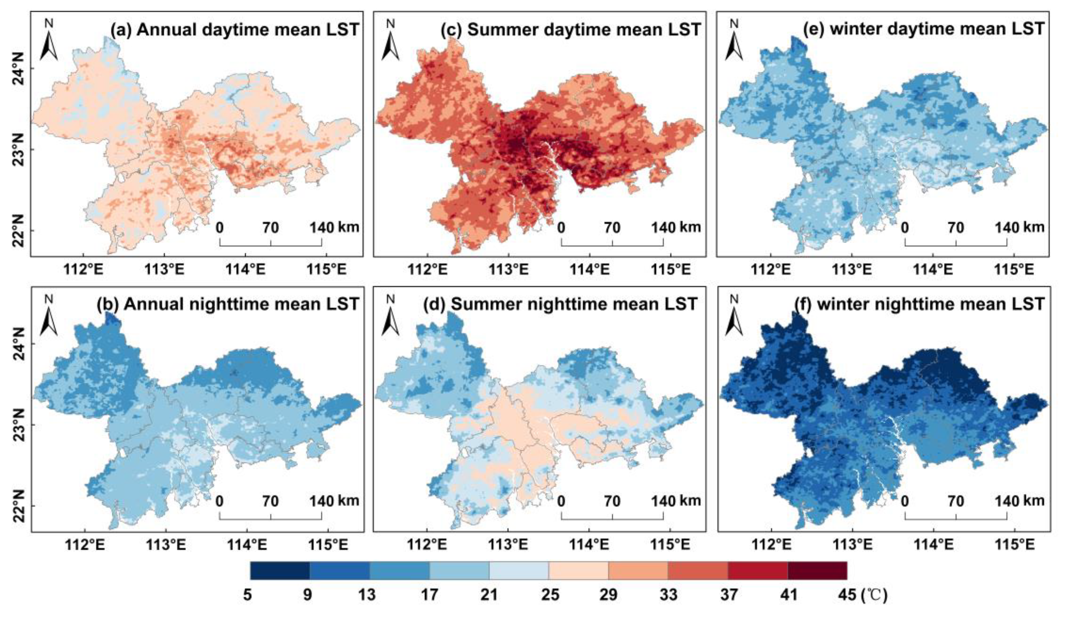
4.2. Spatial Pattern of the LST

The spatial pattern of the LST during daytime and nighttime in summer and winter respectively across BTH, YRD, and PRD is demonstrated in Figure 4, Figure 5, and Figure 6. It can be seen from Figure 4 that central and southern parts of the BTH are dominated by higher LST when compared to northern and northwestern corner of the BTH. However, different LST can be identified during daytime and nighttime in different seasons. Specifically, during the daytime, the average LST of BTH was 20.9 °C. The highest LST was 29.5 °C, while the lowest LST appeared near the mountain was only 3.38 ℃ and the regional LST difference of 26.2 °C. During nighttime, the average LST of BTH was 3.63 °C, and the spatial pattern of the LST is characterized by a strip-shaped pattern following the northeast to southwest direction, and this spatial LST pattern is slightly different from the spatial LST pattern during daytime. Overall, the spatial LST variations during daytime and nighttime in summer and winter are similar, which are consistent with the trend of low in the north and high in the south. But the band shape of the LST distribution at nighttime is more significant. In summer, the maximum LST reached is 44.6 °C during the daytime and the highest is 26.1 °C during the nighttime. By comparing the spatial pattern of LST with Figure 3a and b indicated that the region with higher LST is highly consistent with the IS and higher IS density, corroborating remarkable impacts of urbanization on spatial pattern of LST. In this sense, we can conclude that urbanization can mainly enhance LST changes and the IS is the critical influencing factor behind UHI, which is consistent with the relevant conclusions of previous studies (e.g., Morabito et al. [32]; Guo et al. [38]; Clinton et al. [67]; Zhang et al. [68]; Ravanelli et al. [69]; Cui et al. [70]).
Figure 5 illustrated spatial pattern of LST across the YRD. High LST can be observed mainly concentrated in the central and southern of the YRD, and along the south bank of the Yangtze River and seven urban areas, including Nanjing, Suzhou, Wuxi, Shanghai, Hangzhou, Ningbo and Shaoxing, and also along the Hangzhou Bay, following the “Z” shape, consisting of the spatial pattern of the IS. Spatial pattern of high annual daytime mean LST is similar to that of the summer daytime mean LST. Figure 3c,d and Figure 5 combined to indicate that similar spatial pattern of the LST and IS in particular, showing profound impacts of IS on spatial pattern of LST, evidencing significant impacts of urbanization on changes of LST in both temporal and spatial scales. Meanwhile, the annual nighttime mean LST and the summer nighttime mean LST follow the similar spatial pattern when compared to that of the annual daytime mean LST and summer nighttime mean LST, and the highest nighttime LST is 23.8 °C, and the spatial difference is about 17 °C. The difference is that regions with higher LST than their neighboring regions during the daytime are higher concentrated with clear demarcation when compared to those during the nighttime. Besides, the average LST during annual daytime and nighttime is 18.7 °C and 16.1 °C respectively. The surface UHI during the daytime is enhanced because of reduction in latent heat flux and increase in sensible heat flux as a result of urbanization-induced increased IS [2,12,15]. The latent and sensible heat fluxes are dominant during the daytime, whereas the ground heat fluxes become dominant during the nighttime. During winter nighttime, LST follows no discernable spatial pattern though burry boundaries of high LST can still be observed between urbanized regions and rural regions (Figure 5e,f).
It can be depicted from Figure 6 that spatial pattern of LST across the PRD is similar to the LST across the BTH and YRD. Figure 3e,f and Figure 6 indicated that regions with higher LST than their neighboring regions are mostly those being characterized by high urbanization. The high LST areas are mainly distributed on both banks of the Pearl River Estuary, especially on the east bank of the Pearl River Estuary. And the high LST area have been connected in sheet-like distribution. The Pearl River Estuary is the core area of PRD, which is also the most developed economy and the fastest urbanization process. The annual daytime average LST is higher than the annual nighttime average LST, which are 27.1 °C and 17.8 °C respectively. Compared with the daytime, the high LST area expanded eastwards and northwards respectively during the nighttime with the maximum LST of 26.9 °C and the spatial difference of 11.4 °C. During the winter daytime, the high LST areas spread to the western part of PRD, with the highest temperature of 26.6 °C. During the nighttime, the high LST areas are mainly concentrated in the four urban areas of Dongguan, Shenzhen, Zhongshan, and Zhuhai around the Pearl River Estuary, and the high LST zone moves southern part of PRD, with a maximum temperature of 15.7 °C.

4.3. Relationship Between IS and LST Across the BTH.

Linear relationship was detected between IS and LST (e.g., Estoque et al. [14]). The Pearson correlation coefficient and the determination coefficient between IS density and LST during daytime and nighttime of annual, summer and winter seasons across different cities and urban agglomerations are shown in Figure 7. We found distinctly different relations between LST and IS density across the BTH urban agglomerations (Figure 8a–f) and across the Beijing City (Figure 8g–l). In the figure, each dot represents the LST value corresponding to the IS density in the same grid. The number of images used in each subplot means all LST images. The diurnal and seasonal variations of LST and IS density in different spatial scales of BTH and Beijing were analyzed by using linear regression first. In general, LST increases with the increase of IS density. At the spatial scale of urban agglomeration, there is a significant positive correlation between daytime and nighttime LST and IS density throughout the annual, summer and winter (Figure 7). The Pearson correlation coefficient (r) between LST and IS density during summer was higher than 0.54, which was higher than the annual, while the r value was lowest during winter. The diurnal variations generally show that the daytime correlation is stronger than nighttime. During the summer daytime, the IS contributes the most to the increase of LST, which can explain 37% of the LST increase, while during the winter daytime IS accounts for only 17% of the LST increase. At the spatial scale of individual city, LST and IS density was also significantly positively correlated (Figure 8g–l), the highest r value is 0.88, appeared in the summer daytime, and the IS increase can explain 77% of the LST warming, about twice as much as winter daytime. Although LST during winter nighttime showed a tendency to increase with the increase of IS, the r value was only 0.33 because of the influence such as the ground were frozen and large temperature changes in winter. In conclusion, the warming effect of the IS on the LST of the individual city represented by Beijing is higher than the BTH urban agglomeration, and this warming effect is consistent in the diurnal and seasonal variation, that is higher in summer than in winter and higher in daytime than in nighttime. This means that the IS–LST relations is stronger at the individual city scale. However, at the spatial scale of urban agglomerations, the weaker warming effect of IS on LST is due to the larger spatial structure and size of the urban agglomeration, and the complexity of the underlying surface and climate background, it indicates that it is not only IS that causes changes in LST, but also factors such as vegetation cover, albedo, and climate background [14,15].
Relations between LST and IS density cannot be described by a single linear regression function. It can be easily found from Figure 8a–f that at least two different regression functions should be used to describe relations between LST and IS density with change point at IS density of around 10%. Moreover, this phenomenon is more evident for relations between LST and IS density across the BTH urban agglomerations than the individual Beijing city (Figure 8g–l). Figure 8a–i indicated that one linear regression function along cannot well describe the relations between LST and IS density. Therefore, piecewise linear regression was also adopted when linear regression cannot better describe the relationship between LST and IS density. It can be seen from Figure 8 that sharp increase of LST can be detected, given the increase in IS density under the condition that IS density is smaller than about 10%. When IS density is larger than about 10%, the increase of LST will slow down. The major cause behind the UHI is the reduction of latent heat flux but increase in sensible heat due to increase of IS density. In this study, the IS density is calculated using the kernel density estimation, which indicates the density of the IS in its surrounding pixels. Increase of IS density means from rural area to urbanized area. Increase of IS density from 0% to about 10% can strongly increase LST and the increase of LST slows down when the IS density more than about 10%. It indicates that the change rate of LST is related to the IS density, at the initial stage when IS density increases, LST increases at a faster rate. However, with the increase of IS density, the increase rate of LST slightly slows down. When the IS density reaches a certain degree, the impact on the thermal environment will be further reduced. Therefore, relations between LST and IS density are not linear in a rigorous sense (Figure 8) [34,38]. In addition, because of the difference in environmental effects of different underlying surface features, relationships between the IS density and the LST are also heavily influenced by selections of the pixel sizes. Shifting relations can be expected between LST and IS density given different pixel sizes [71]. When the IS density is greater than about 17% during the daytime of winter, the increase of the LST with increase of the IS density slightly slows down and even negative relations between LST and IS density. At the beginning of the IS density increased, the LST increases with IS. However, there are more dry and cold bare soil without vegetation distribution in winter, specific heat capacity of dry and cold bare soil surface is lower than the IS. As a result, the temperature of IS rise at a slower rate than the surrounding non-IS during the cold winter, leading to the “cooling effect” [58]. This phenomenon is consistent with Figure 4e, it is not significant that urban areas LST is higher than the surrounding areas during the winter daytime. Therefore, the effect of IS on the LST is reduced. In addition, the high thermal inertia of the building materials and the shade effect of the high building which is similar to the cooling effects of the vegetation, reducing the warming effect of IS on LST in winter [19,72].

4.4. Relationship Between IS and LST Across the YRD

We evaluated the relations between LST and IS density across the YRD urban agglomeration (Figure 9a–f) and the Shanghai City (Figure 9g–l). The LST and IS density is positively correlated with significant diurnal changes and seasonal variability (Figure 9). We also found the correlation between IS and LST during the daytime is much higher than nighttime, the r value is about 2.5 times larger than nighttime. Similarly, the relationship between IS and LST reach the strongest during the daytime in summer, the r value is about three times larger than winter daytime (Figure 7a). In addition, Figure 7a indicated the weak r value between LST and IS density during nighttime of winter and the r value is 0.02. Similar findings were obtained in analysis of relations between LST and IS density in relevant studies [5,23]. At diurnal scale, the relationship between LST and IS density is more significant during the daytime than during the nighttime with correlation coefficient of 0.69, which can explain 49% of the increase in the LST throughout the year. In the summer daytime, the r value between LST and IS density is the highest, being 0.72. The increase of the IS can explain 52.4% of the LST increase. While, the r value between LST and IS density during the winter nighttime is just 0.0003.
Shanghai is a metropolis on the alluvial plains of the YRD. Since the 1990s, the population has increased dramatically with rapidly growing GDP and accelerated urbanization [73]. Relationship between LST and IS density is illustrated in Figure 9g–l. It can be seen from Figure 9 that the IS density of the Shanghai City is concentrated between 20%–80%, indicating fast land use and land cover changes from natural land to the IS. In general, the increase of IS can trigger the increase of LST. We found the higher r value between LST and IS density during daytime than nighttime. The r value between LST and IS density during daytime is 2.5 times larger than during nighttime. The IS increase during daytime can explain 51% of the LST changes, being higher than during nighttime which can explain 8% of the LST changes [73,74]. In the urbanized area, characteristics of the underlying surface differentiate the thermal effects of IS. The specific heat capacity of IS is larger, which refers to the heat absorption and heat storage ability of the IS are both stronger, making it more effective to store solar energy as heat and storing more energy. Because of the coverage of IS, the heat absorption is faster during the daytime, leading to the LST is higher than during the nighttime. Therefore, the warming effect of the IS is stronger during daytime than during nighttime [75]. From the seasonal perspective, the relationship between LST and IS density is the strongest during summer daytime with correlation coefficient of 0.81, being about three times larger than that during winter daytime, can explain 66% of the LST increase. This is because the solar radiation is stronger in summer than in other seasons. Solar radiation enters the atmosphere, most of solar radiation can reach the ground surface through the atmosphere, which heats the ground surface and intensifies the UHI. Besides, the daytime in summer are longer and the heating effect of solar radiation is more pronounced. Moreover, human emission of heat can also enhance LST changes. Therefore, the impacts of IS on LST are stronger during summer than during winter. Similarly, the correlation between LST and IS density in Nanjing and Hangzhou (Figure 7a) is strongest in summer and is higher during daytime than during nighttime. Comparison of the relationship between LST and IS density over individual cities and urban agglomerations indicate that weakening impacts of IS can be observed on UHI given large spatial scale.

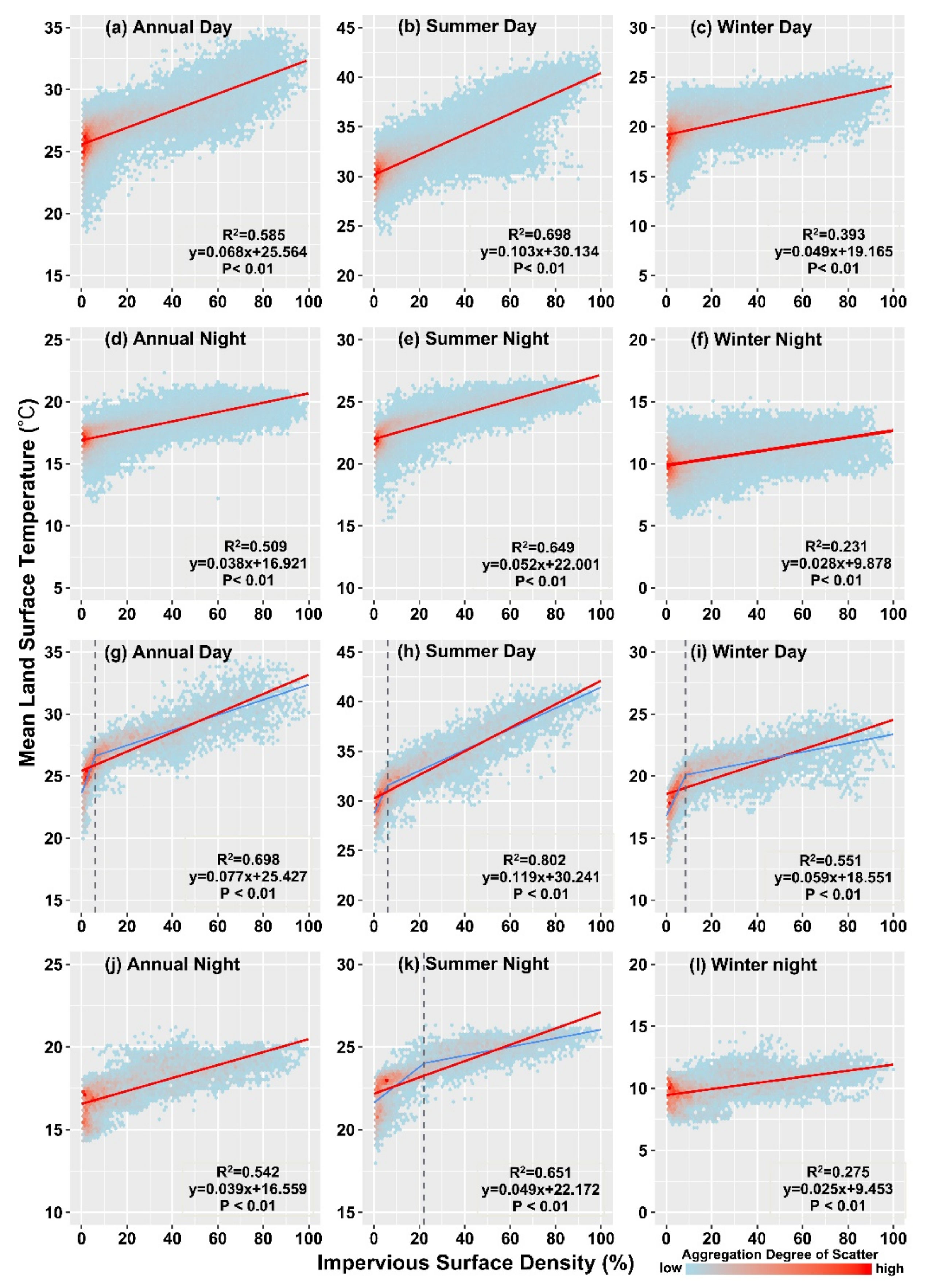
4.5. Relationship Between is and LST Across the PRD

We evaluated the relations between LST and IS density across the PRD (Figure 10a–f) and the Guangzhou City (Figure 10g–l). Linear relation can be detected between LST and IS density. At the spatial scale of the PRD urban agglomeration, increase of the IS density during summer and annual time interval can explain more than 50% of the LST increase. The r values and coefficient of determination (R2) are the highest during the summer daytime (Figure 7), being respectively 0.83 and 0.70. In winter, the correlation between LST and IS density is relatively weak. The r value between LST and IS density during the daytime is 0.63, which can explain 39% of the increase in LST. The r value between LST and IS density during nighttime is only 0.48. We found the highest r value between LST and IS density during summer daytime and the lowest correlation coefficient between LST and IS density during winter nighttime, being 0.89 and 0.53 respectively across the Guangzhou City (Figure 7a). Increase in IS density can explain 80% of increase in LST. On the contrary, the R2 value of the linear regression between LST and IS density is the lowest during winter nighttime, and IS density changes can only explain 28% of the LST changes. Similarly, the R2 value and r value between LST and IS density across the Dongguan and Shenzhen follow above-mentioned changing pattern (Figure 7). However, except winter nighttime, the correlation coefficient and coefficient of determination between LST and IS density across individual city are all higher than those across urban agglomerations. In addition, when the IS density in Guangzhou is about 8% during the daytime, the relationship between the IS density and the LST is segmented, indicating more complicated mechanisms behind relations between IS density and the LST. For example, cell sizes of the IS and LST data selected in the research, different cell sizes will lead to the difference in IS–LST relations [58]. Moreover, The LST increases faster in the initial period of IS increase, and when the IS density reaches a certain level, its further increase will reduce the impact on the urban thermal environment [38].

4.6. Relationship between other Factors than IS Density on LST Changes

Aforementioned results indicated different enhancement effects of the IS density on LST changes in different cities, urban agglomerations located along different latitudes, which implied that IS was not the only driving factors behind LST changes. Vegetation, albedo, and climatic variables are believed to be the driving factors behind UHI [15]. In this case, we considered other potential driving factors such as NDVI, albedo, air temperature, precipitation and altitude, and so on. We used the multivariate stepwise regression and AIC criteria to screen out major driving factors. Furthermore, we used the multiple GLM (the general linear model) to quantify the fractional contributions of these potential driving factors to LST changes (Figure 11). Besides, we also analyzed the relationship between LST and NDVI, albedo, air temperature, precipitation, and altitude using r (Figure 12). It can be seen from Figure 11 that the contribution of various influencing factors to LST changes varies temporally from one region to another. Among these five factors, i.e., NDVI, albedo, air temperature, precipitation, and altitude, the contribution of NDVI to LST change is the highest, up to 79.39%. However, this contribution of NDVI to LST varies in both spatial and temporal time. During the summer daytime, the impacts of vegetation on LST changes are generally appreciable, while during the winter nighttime, vegetation has a lower contribution rate to the LST change, with a minimum of 0.34%.In addition, there is a significant negative correlation between vegetation and LST (Figure 12), and this negative correlation becomes weaker with increased spatial scale. Impacts of vegetation on LST are more significant during summer than during winter. Because of better vegetation conditions during summer than during winter, the transpiration of vegetation is stronger during summer than during winter. Therefore, the cooling effects of vegetation on the LST are stronger in summer than that in winter. The diurnal variation of impacts of vegetation on LST changes shows higher correlation between vegetation and LST during daytime than during nighttime, which can be attributed to the cooling effect of the vegetation on LST which is stronger during the daytime than during the nighttime, because of stronger vegetation transpiration at daytime than at nighttime [58]. Moreover, the cooling effect of vegetation on LST during different seasons and times can also be affected by environmental temperature [76].
The impacts of albedo on LST change are generally lower than vegetation. Besides, this kind of influence is lower during summer than during winter. The contribution of albedo to LST is the highest of 47.58% during winter daytime and is the lowest of 0.0001% during summer nighttime. In addition, the albedo is in stronger correlation with increase of LST during daytime than during nighttime (Figure 12). Moreover, the correlation between albedo and LST is relatively lower during summer nighttime than during summer daytime. During summer, vegetation conditions are better than during winter which absorb more solar radiation during summer than during winter [77]. Besides, comparatively higher cloud coverage and higher relative humidity during summer than during winter is also another reason behind lower contribution of albedo to LST changes during summer than during winter. Comparatively, worse vegetation condition but more bare soils and possible snow coverage during winter all enhance albedo and hence larger contribution of albedo to LST changes during winter than during summer [12].
The relations between air temperature and LST are heavily modulated by underlying surface properties, weather conditions, and even cloud coverage [78]. According to Zhu et al. [79], the energy exchange between the atmosphere and the underlying surface affects LST changes, and hence there exists certain impact of air temperature on LST variations and specifically the air temperature changes tend to drive increase of LST. The contribution rate of air temperature to LST shifts in both temporal and spatial scales. For example, in BTH, the annual and seasonal contribution of air temperature to the change of LST is relatively high, and the highest contribution rate is 78.82% during summer nighttime, the lowest contribution of air temperature to LST is 24.14% during summer daytime. Furthermore, we found higher correlation between air temperature and LST during summer than during winter (Figure 12), indicates significant impacts of air temperature on LST during summer. In addition, we also found remarkable diurnal difference in the impacts of air temperature on LST, but no obvious spatial and temporal regularity was detected, indicating impacts of other driving factors than air surface on LST such as underlying surface properties, weather conditions and even cloud cover [79]. Precipitation has the lowest contribution to LST change, and the contribution rate ranges between 0 to 5%. The highest contribution of precipitation of 8.97% to LST changes was observed during summer nighttime. Precipitation is mainly in negative correlations with LST changes (Figure 12). Cooling effects of precipitation on LST are mainly by soil moisture changes. More precipitation triggers higher soil moisture and vice versa. Soil moisture changes can cause changes in latent heat and sensible heat and hence LST variations [80].
The contribution of altitude changes to LST variations is slightly higher than the contribution of precipitation to LST change. Impacts of altitude changes on LST variations vary in both spatial and temporal scales with the contribution ranging between 0 to 16% and the highest contribution of altitude to LST is 15.8%. We found decrease of LST with increase of altitude (Figure 12). Besides, altitude changes have stronger impacts on LST changes during summer than during winter. Aforementioned analysis results indicated complicated driving factors behind LST changes. The IS density is the critical driving factor behind LST changes in both spatial and temporal scales. However, impacts of other factors than IS density can also have remarkable impacts on LST changes such as precipitation, vegetation conditions, albedo and so on.

5. Discussions

5.1. Accuracy of MODIS LST Data

There have been many studies on the validation of MODIS LST data in recent decades. First of all, the LST data observed by the in-situ measurements can be used to verify the MODIS LST data [50,52], comparing ground infrared temperature radiation data with MODIS LST data. Wan et al. improved MODIS LST products by relevant correcting noise, in order to acquire more high-quality data in the LST products and minimize cloud contamination. By comparing between Version 5 MODIS LSTs and in situ values indicate that the accuracy of the MODIS LST product is better than 0.5 K for all 39 clear-sky cases [52]. Wang et al. found that the MODIS LST datasets at 1–km resolution were consistent well with the ground-based LST measurements, with a standard deviation of 0.84 K [81], and proved that MODIS LST products can be used in UHI research [51]. Moreover, using surface longwave radiation observations to verify the accuracy of MODIS LST data [82]. Rigo et al. confirmed a high correlation of the long wave emissions measured by the satellite and the in–situ measurements, with an accuracy of ±3% to 5% on average between in–situ measurements and MODIS LST data, and demonstrated the accuracy of MODIS LST data for urban area research [50]. Wang et al. evaluated MODIS LST products using long-term surface longwave radiation observations collected at six sites, and the results showed that the MODIS LST retrieval agreed well with ground-based measurements, the average bias is −0.2 °C [83].
The research on the validation of MODIS LST data in China and worldwide is as follows. Wan et al. conducted quality assessment and verification of MODIS global LST data, and the results showed that using both Terra and Aqua MODIS data in LST retrieval greatly improves data quality [84]. Chen et al. made the comparison between in situ and MODIS monthly LST worldwide, and found that the mean bias of MODIS LST data is less than 0.59, which can all provide a reliable estimate of all-sky monthly mean LST [85]. Gao et al. carried out China MODIS LST products verification, the results showed that the accuracy of the MODIS LST products is very high, which is suitable for the study of the spatial distribution of surface heat in large and mesoscale regions [86]. Moreover, there are many studies based on MODIS LST data (MOD11A2 and MYD11A2) with focus on the Beijing–Tianjin–Hebei [12,15,58,87], Yangtze River Delta [2,12,58,88] and Pearl River Delta [12,58,89], which fully demonstrate the applicability of the accuracy of the MODIS LST data in this study area. In conclusion, the high accuracy of MODIS LST products is sufficient for the UHI research [15,38,58].

5.2. Time-Scale Differences in the Effects of IS on LST

In the above-mentioned studies, we displayed the relationships between LST and IS density during six different temporal scales, daytime and nighttime of annual year, summer and winter (Figure 7). In terms of diurnal and seasonal relationships between LST and IS density, the relationship is positively linear, i.e., increase of IS tends to enhance LST, the positive relationship is consistent with the results of previous studies in the same study area [5,36,90,91]. Therefore, the IS density changes is the critical driving factor behind LST changes, modifying ground surface energy balance and driving LST variations in both temporal and spatial scales [12]. The increased IS impedes infiltration processes, reduces soil moisture content and water vapor evaporating from soil and vegetation, and reduces latent heat fluxes through the urbanized areas and boundary layers. The IS are mostly artificial cement pavements, plastic materials and related man-made building materials, which have strong solar radiation absorption capacity and hence can alter LST variations in both spatial and temporal scales [12,37]. In terms of diurnal variation, the IS changes can explain as high as 86% of the changes in LST variations during summer daytime, while the coefficient of determination of relations between LST and IS density during winter nighttime can be as low as 0.0003. This means that the IS–LST relations became stronger during daytime than nighttime, which can be explained by the strong solar radiation during daytime. Moreover, the IS has a larger specific heat capacity and the increase of IS also makes the thermal conductivity of the surface ground increase, which results in faster heat absorption during the daytime and the warming effect of IS on LST is stronger than that during the nighttime [72,75]. However, the correlation between LST and IS density in some specific cities is higher during the nighttime than the daytime. This means the IS has a stronger impact on LST during nighttime in these specific cities [58], which attributed to the fact that the local city is highly vegetated. During daytime, the vegetation reduces the LST by latent heat flux, while vegetation transpiration is reduced during nighttime. As a result, the cooling effect of the vegetation is weakened and the IS enhances LST changes during nighttime when compared to that during daytime [72]. As studied by Peng et al. [92], seasonal differences in UHI existed in 98.8% of cities over the China. For the seasonal difference in the relationship between IS and LST, our study indicates the IS has more significant impacts on LST during summer than winter, indicating that the IS can explain the LST better in summer than in winter, which is consistent with the research results of Ma et al. [58]. This is mainly due to the difference in solar radiation between summer and winter. In summer, the solar radiation is strong and the daylight hours are long, which are beneficial for the IS to the absorption of solar radiation, leading to a stronger relationship between IS density and LST during summer.

5.3. Spatial-Scale Differences in the Effects of IS on LST

With the development of urbanization, the distance between cities continues to shrink and even disappear. In this way, urban agglomerations are formed. Increasing the surface temperature of a continuous large area in an urban agglomeration changes the regional thermal environment, which leads to more serious UHI [2]. This article not only studies the warming effect of IS on LST in an individual city and urban agglomeration, but also compares the spatial difference of the IS–LST relations. From a perspective of spatial scale, the IS has more significant impacts on the rise of LST across the individual city than across the urban agglomeration [58]. Moreover, we observed different correlation coefficients between LST and IS density across different urban agglomerations, e.g., BTH, YRD, and PRD in this current study. The correlation coefficients between LST and IS density across the Beijing City, the Shanghai City and the Guangzhou City is 2.5 times, 1.1 times, and 1.07 times larger than those across the BTH, YRD and PRD urban agglomeration respectively. The above research results showed the difference in the relationship between IS and LST in an individual city and urban agglomeration, which is consistent with the conclusion that the UHI intensity is closely related to city size studied by Zhou et al. [93]. At the individual city scale, we found higher correlation between LST and IS density than at urban agglomeration scale, probably because the underlying surface of the urban region is mainly composed of IS. Such surface composition and underlying structure make the LST highly affected by the IS changes. Moreover, IS such as buildings and roads are mainly composed of dark surfaces, which absorb a large amount of heat, resulting in an obvious increase in LST [13]. As for urban agglomeration, weak impacts of IS on LST changes should be due to complicated ground surface properties and urban structure and complex local urban climate as well. In this case, the influencing factors for LST changes are not limited to IS, influencing factors also include vegetation coverage, albedo and local climates [14,15]. In addition, there are many cities within the urban agglomerations, and some cities are close to mountains or water bodies. Because of the regulation of valley winds, sea, and land breeze, the enhancement effects of IS on LST changes temperature will be relatively weakened. Therefore, in the larger spatial scale, the effect of IS on the LST is weak. The relationship between IS and surface temperature is stronger for individual urban area than for urban agglomerations, implying that the IS can highly affect LST changes at smaller spatial scale or from viewpoint of individual urban area [58]. Meanwhile, we found distinct spatial heterogeneity for IS that has different impacts on LST changes across BTH. There is a positive correlation between IS density and LST in BTH, but the relationship is piecewise linear. This is consistent with the research results of Guo et al. about the influence of IS on LST in Beijing area [38]. At the beginning of the increase of IS, the LST rises rapidly When the IS density reaches a certain proportion, the LST increases linearly and slowly.
For the three urban agglomerations, comparison of the correlation between LST and IS density within the three major urban agglomerations helps to find that the correlation coefficients between LST and IS density within BTH is the smallest during six time periods considered in this study, i.e., summer daytime/nighttime, winter daytime/nighttime, annual daytime/nighttime, and is followed by the correlation coefficients between LST and IS density within YRD and PRD. While, we found consistency in relations between LST and IS within three urban agglomerations considered in this study, i.e., the larger the spatial scale, the weaker the enhancement effects of the IS on LST changes, and vice versa. In addition, according to the research of Peng et al. [15], the UHI is strongly influenced by climatic background. The BTH, the YRD, and the PRD are located in the north, middle east, and south of China, respectively. Because of the different latitudes and geographical locations of the three urban agglomerations, the climate types are also different. From the north to south is the temperature monsoon climate, subtropical marine climate and humid subtropical monsoon climate, with different relative humidity, air temperature and vegetation coverages [31], hence driving differences in the enhancement effect of the IS on the LST within these three major urban agglomerations. The underlying surface conditions and climatic conditions of urban agglomerations are complex. Therefore, there are many influencing factors cause differences in the warming effect of IS on LST, which needs to be further explored in the future.

6. Conclusions

In this current study, we focused on quantifying relations between IS density and LST at different spatiotemporal scales, spatial size, and climate conditions, and attempted to investigate the IS–LST relations changes across individual cities and urban agglomerations. Moreover, in order to further explore the factors affected LST, we quantify the contribution rates of NDVI, albedo, DEM and climate background to LST. We draw the following conclusions.
(1)
In terms of temporal scale, the warming effect of IS on LST generally stronger in daytime than in nighttime and significantly stronger in summer than winter.
(2)
From the perspective of spatial scale, as for the individual city, the IS density has high impacts, indicating that IS can better reflect the change of LST at the individual city scale. Within the urban agglomerations, IS density has less significant impacts on LST, comparing to individual city. This is because larger spatial size includes more complicated underlying components and spatial structures, leading to the relative weakening of the IS–LST relations.
(3)
The differences in spatial sizes, latitude locations, and climate background over the three urban agglomerations in this study, resulting the differences in IS–LST relations between urban agglomerations. Linear relations cannot well describe the IS–LST relations in the BTH, with IS density appearing in segments between about 10% to 17%. This phenomenon indicates the IS density reaches a certain level, the impact on the thermal environment will be further reduced. Moreover, because of the different spatial sizes and climatic backgrounds of the three urban agglomerations, we observed that urban agglomerations are distributed from north to south in China, and the warming effect of IS on LST has gradually increased.
(4)
The relationships between IS and LST vary in both spatial and temporal scales, which indicates that LST is not only affected by IS density, but also affected by other driving factors such as precipitation, DEM, vegetation coverage, albedo, and temperature. Based on quantification of the driving factors behind LST, we found that the contribution rate of vegetation to LST was generally higher, followed by albedo. The heat exchange between the atmosphere and the surface will affect the change of LST, so the air temperature has a certain degree of positive driving on LST. The contribution of precipitation to LST is the lowest in this study area, and the impact of DEM on LST is slightly higher than precipitation.

Author Contributions

Conceptualization, Q.Z.; formal analysis, Q.Z. and Z.W.; funding acquisition, Q.Z.; investigation, Q.Z. and Z.W.; software, Z.W.; supervision, Q.Z.; validation, Z.W.; writing—original draft, Q.Z.; writing—review and editing, Q.Z., H.Y., X.Z., and Z.S. All authors have read and agreed to the published version of the manuscript.

Funding

This research has been financially supported by the National Science Foundation of China, Grant No. 41771536, the China National Key R&D Program, Grant No. 2019YFA0606900, and the National Science Foundation for Distinguished Young Scholars of China, Grant No. 51425903.

Acknowledgments

Our cordial gratitude should be extended to the editor, Mladen Radosavljević, and anonymous reviewers for their professional comments and pertinent suggestions which are greatly helpful for further quality improvement of this current manuscript.

Conflicts of Interest

The authors declare no conflict of interest.

References

  1. Zhou, X.F.; Chen, H. Impact of urbanization-related land use land cover changes and urban morphology changes on the urban heat island phenomenon. Sci. Total Environ. 2018, 635, 1467–1476. [Google Scholar] [CrossRef] [PubMed]
  2. Du, H.Y.; Wang, D.D.; Wang, Y.Y.; Zhao, X.L.; Qin, F.; Jiang, H.; Cai, Y.L. Influences of land cover types, meteorological conditions, anthropogenic heat and urban area on surface urban heat island in the Yangtze River Delta Urban Agglomeration. Sci. Total Environ. 2016, 571, 461–470. [Google Scholar] [CrossRef] [PubMed]
  3. Zhao, L.; Lee, X.H.; Smith, R.B.; Oleson, K. Strong contributions of local background climate to urban heat islands. Nature. 2014, 511, 216–219. [Google Scholar] [CrossRef] [PubMed]
  4. Owen, T.W.; Carlson, T.N.; Gillies, R.R. An assessment of satellite remotely-sensed land cover parameters in quantitatively describing the climatic effect of urbanization. Int. J. Remote Sens. 1998, 19, 1663–1681. [Google Scholar] [CrossRef]
  5. Yuan, F.; Bauer, M.E. Comparison of impervious surface area and normalized difference vegetation index as indicators of surface urban heat island effects in Landsat imagery. Remote Sens. Environ. 2007, 106, 375–386. [Google Scholar] [CrossRef]
  6. Kalnay, E.; Cai, M. Impact of urbanization and land-use change on climate. Nature 2003, 423, 528–531. [Google Scholar] [CrossRef] [PubMed]
  7. Zhou, L.; Dickinson, R.E.; Tian, Y.; Fang, J.; Li, Q.; Kaufmann, R.K.; Tucker, C.J.; Myneni, R.B. Evidence for a significant urbanization effect on climate in china. Proc. Natl. Acad. Sci. USA 2004, 101, 9540–9544. [Google Scholar] [CrossRef] [Green Version]
  8. United Nations. Department of Economic and Social Affairs, Population Division, World Population Prospects: The 2010 Revision, Volume I: Comprehensive Tables. 2011. Available online: https://www.un.org/en/development/desa/publications/world-population-prospects-the-2010-revision.html (accessed on 3 May 2020).
  9. Zhu, X.D.; Zhang, Q.; Sun, P.; Singh, V.P.; Shi, P.J.; Song, C.Q. Impact of urbanization on hourly precipitation in Beijing, China: Spatiotemporal patterns and causes. Glob. Planet. Change 2019, 172, 307–324. [Google Scholar] [CrossRef]
  10. Reid, W.V. Biodiversity hotspots. Trends Ecol. Evol. 1998, 13, 275–280. [Google Scholar] [CrossRef]
  11. Gong, P.; Liang, S.; Carlton, E.J.; Jiang, Q.; Wu, J.; Wang, L.; Remais, J.V. Urbanization and health in China. Lancet 2012, 379, 843–852. [Google Scholar] [CrossRef]
  12. Zhou, D.C.; Zhao, S.Q.; Liu, S.G.; Zhang, L.X.; Zhu, C. Surface urban heat island in China’s 32 major cities: Spatial patterns and drivers. Remote Sens. Environ. 2014, 152, 51–61. [Google Scholar] [CrossRef]
  13. Yang, J.C.; Hu, L.Q.; Wang, C.H. Population dynamics modify urban residents’ exposure to extreme temperatures across the United States. Sci. Adv. 2019, 5, eaay3452. [Google Scholar] [CrossRef] [PubMed] [Green Version]
  14. Estoque, R.C.; Murayama, Y.; Myint, S.W. Effects of landscape composition and pattern on land surface temperature: An urban heat island study in the megacities of Southeast Asia. Sci. Total Environ. 2017, 577, 349–359. [Google Scholar] [CrossRef] [PubMed]
  15. Peng, S.S.; Piao, S.L.; Ciais, P.; Friedlingstein, P.; Ottle, C.; Bréon, F.M.; Nan, H.J.; Zhou, L.M.; Myneni, R.B. Surface urban heat island across 419 global big cities. Environ. Sci. Technol. 2012, 46, 696–703. [Google Scholar] [CrossRef]
  16. Chow, W.T.L.; Roth, M. Temporal dynamics of the urban heat island of Singapore. Int. J. Climatol. 2006, 26, 2243–2260. [Google Scholar] [CrossRef]
  17. Azevedo, J.A.; Chapman, L.; Muller, C.L. Quantifying the daytime and night-time urban heat island in Birmingham, UK: A comparison of satellite derived land surface temperature and high resolution air temperature observations. Remote Sens. 2016, 8, 153. [Google Scholar] [CrossRef] [Green Version]
  18. Li, H.D.; Zhou, Y.Y.; Li, X.M.; Meng, L.; Wang, X.; Wu, S.; Sodoudi, S. A new method to quantify surface urban heat island intensity. Sci. Total Environ. 2018, 624, 262–272. [Google Scholar] [CrossRef]
  19. Myint, S.W.; Wentz, E.A.; Brazel, A.J.; Quattrochi, D.A. The impact of distinct anthropogenic and vegetation features on urban warming. Landsc. Ecol. 2013, 28, 959–978. [Google Scholar] [CrossRef] [Green Version]
  20. Kourtidis, K.; Georgoulias, A.K.; Rapsomanikis, S.; Amiridis, V.; Keramitsoglou, I.; Hooyberghs, H.; Melas, D. A study of the hourly variability of the urban heat island effect in the Greater Athens Area during summer. Sci. Total Environ. 2015, 517, 162–177. [Google Scholar] [CrossRef] [Green Version]
  21. Tran, D.X.; Pla, F.; Latorre-Carmona, P.; Myint, S.W.; Caetano, M.; Kieu, H.V. Characterizing the relationship between land use land cover change and land surface temperature. ISPRS J. Photogramm. Remote Sens. 2017, 124, 119–132. [Google Scholar] [CrossRef] [Green Version]
  22. Majkowska, A.; Kolendowicz, L.; Półrolniczak, M.; Hauke, J.; Czernecki, B. The urban heat island in the city of Poznań as derived from Landsat 5 TM. Theor. Appl. Climatol. 2016, 128, 1–15. [Google Scholar] [CrossRef] [Green Version]
  23. Imhoff, M.L.; Zhang, P.; Wolfe, R.E.; Bounoua, L. Remote sensing of the urban heat island, effect across biomes in the continental USA. Remote Sens. Environ. 2010, 114, 504–513. [Google Scholar] [CrossRef] [Green Version]
  24. Song, J.; Du, S.H.; Feng, X.; Guo, L. The relationships between landscape compositions and land surface temperature: Quantifying their resolution sensitivity with spatial regression models. Landsc. Urban Plan. 2014, 123, 145–157. [Google Scholar] [CrossRef]
  25. Cheval, S.; Dumitrescu, A. The summer surface urban heat island of Bucharest (Romania) retrieved from MODIS images. Theor. Appl. Climatol. 2015, 121, 631–640. [Google Scholar] [CrossRef]
  26. Arnold, C.L.; Gibbons, C.J. Impervious surface coverage: The emergence of a key environmental indicator. J. Am. Plan. Assoc. 1996, 62, 243–258. [Google Scholar] [CrossRef]
  27. Weng, Q.H. Remote sensing of impervious surfaces in the urban areas: Requirements, methods, and trends. Remote Sens. Environ. 2012, 117, 34–49. [Google Scholar] [CrossRef]
  28. Arnfield, A.J. Two decades of urban climate research: A review of turbulence, exchanges of energy and water, and the urban heat island. Int. J. Climatol. 2003, 23, 1–26. [Google Scholar] [CrossRef]
  29. Oke, T.R. The energetic basis of the urban heat island. Q. J. R. Meteorol. Soc. 1982, 108, 1–24. [Google Scholar] [CrossRef]
  30. Meng, Q.Y.; Zhang, L.L.; Sun, Z.H.; Meng, F.; Wang, L.; Sun, Y.X. Characterizing spatial and temporal trends of surface urban heat island effect in an urban main built-up area: A 12-year case study in Beijing, China. Remote Sens. Environ. 2017, 204, 826–837. [Google Scholar] [CrossRef]
  31. Rhee, J.Y.; Park, S.Y.; Lu, Z.Y. Relationship between land cover patterns and surface temperature in urban areas. GISci. Remote Sens. 2014, 51, 521–536. [Google Scholar] [CrossRef]
  32. Morabito, M.; Crisci, A.; Messeri, A.; Orlandini, S.; Raschi, A.; Maracchi, G.; Munafo, M. The impact of built-up surfaces on land surface temperatures in Italian urban areas. Sci. Total Environ. 2016, 551, 317–326. [Google Scholar] [CrossRef] [PubMed]
  33. Sun, Q.Q.; Wu, Z.F.; Tan, J.J. The relationship between land surface temperature and land use/land cover in Guangzhou, China. Environ. Earth Sci. 2012, 65, 1687–1694. [Google Scholar] [CrossRef]
  34. Xu, H.Q.; Lin, D.F.; Tang, F. The impact of impervious surface development on land surface temperature in a subtropical city: Xiamen, China. Int. J. Climatol. 2013, 33, 1873–1883. [Google Scholar] [CrossRef]
  35. Ding, H.Y.; Shi, W.Z. Land-use/land-cover change and its influence on surface temperature: A case study in Beijing City. Int. J. Remote Sens. 2013, 34, 5503–5517. [Google Scholar] [CrossRef]
  36. Guo, G.H.; Wu, Z.F.; Xiao, R.B.; Chen, Y.B.; Liu, X.N.; Zhang, X.S. Impacts of urban biophysical composition on land surface temperature in urban heat island clusters. Landsc. Urban Plan. 2015, 135, 1–10. [Google Scholar] [CrossRef]
  37. Kuang, W.H.; Liu, Y.; Dou, Y.Y.; Chi, W.F.; Chen, G.S.; Gao, C.F.; Yang, T.R.; Liu, J.Y.; Zhang, R.H. What are hot and what are not in an urban landscape: Quantifying and explaining the land surface temperature pattern in Beijing, China. Landsc. Ecol. 2015, 30, 357–373. [Google Scholar] [CrossRef]
  38. Guo, L.J.; Liu, R.M.; Men, C.; Wang, Q.R.; Miao, Y.X.; Zhang, Y. Quantifying and simulating landscape composition and pattern impacts on land surface temperature: A decadal study of the rapidly urbanizing city of Beijing, China. Sci. Total Environ. 2019, 654, 430–440. [Google Scholar] [CrossRef]
  39. Xie, H.L.; He, Y.F.; Xie, X. Exploring the factors influencing ecological land change for China’s Beijing-Tianjin-Hebei Region using big data. J. Clean Prod. 2017, 142, 667–687. [Google Scholar] [CrossRef]
  40. Shi, Y.; Jiang, Z.H.; Dong, L.P.; Shen, S.H. Statistical Estimation of High-Resolution Surface Air Temperature from MODIS over the Yangtze River Delta, China. J. Meteorol. Res. 2017, 2, 190–196. [Google Scholar] [CrossRef]
  41. Hu, D.K.; Clift, P.D.; Boning, P.; Hannigan, R.; Hillier, S.; Blusztajn, J.; Wan, S.M.; Fuller, D.Q. Holocene evolution in weathering and erosion patterns in the Pearl River delta. Geochem. Geophys. Geosyst. 2013, 14, 2349–2368. [Google Scholar] [CrossRef] [Green Version]
  42. Xiao, J.C.; Yuan, Z. The Top Ten Urban Agglomerations in China; Economic Science Press: Beijing, China, 2009; pp. 363–367. [Google Scholar]
  43. Shao, Y.H.; Wu, J.M.; Ye, J.Y.; Liu, Y.H. Frequency analysis and its spatiotemporal characteristics of precipitation extreme events in China during 1951-2010. Theor. Appl. Climatol. 2015, 121, 1–13. [Google Scholar] [CrossRef]
  44. Wang, J.; Zhou, W.Q.; Xu, K.P.; Yan, J.L. Spatiotemporal pattern of vegetation cover and its relationship with urbanization in Beijing-Tianjin-Hebei megaregion from 2000 to 2010. Acta Ecol. Sinica 2017, 37, 7019–7029. [Google Scholar]
  45. Jia, Y.Q.; Zhang, B.; Zhang, Y.Z.; Tang, M.; Ma, B.; Wang, G.Q.; Liu, X.L.; Luo, Z.M. Effect of urbanization on spatial and temporal variation of extreme temperature events in the Yangtze River Delta. J. Nat. Resour. 2017, 32, 814–828. [Google Scholar]
  46. Li, R.J. Discussion on the gains and losses of urbanization in the Pearl River Delta—Analysis based on the census data. Popul. Econ. 2014, 1, 15–18. [Google Scholar]
  47. Xu, H.Q.; Wang, M.H. Remote sensing-based retrieval of ground impervious surfaces. J. Remoting Sens. 2016, 20, 1993–2002. [Google Scholar]
  48. Madhavan, B.B.; Kubo, S.; Kurisaki, N.; Sivakumar, T.V.L.N. Appraising the anatomy and spatial growth of the bangkok metropolitan area using a vegetation-impervious-soil model through remote sensing. Int. J. Remote Sens. 2001, 22, 789–806. [Google Scholar] [CrossRef]
  49. Wan, Z.M.; Dozier, J. A generalized split-window algorithm for retrieving land-surface temperature from space. IEEE Trans. Geosci. Remote Sens. 1996, 34, 892–905. [Google Scholar]
  50. Rigo, G.; Parlow, E.; Oesch, D. Validation of satellite observed thermal emission with in-situ measurements over an urban surface. Remote Sens. Environ. 2006, 104, 201–210. [Google Scholar] [CrossRef]
  51. Wang, K.C.; Wang, J.K.; Wang, P.C.; Sparrow, M.; Yang, J.; Chen, H.B. Influences of urbanization on surface characteristics as derived from the Moderate-Resolution Imaging Spectroradiometer: A case study for the Beijing metropolitan area. J. Geophys. Res. Atmos. 2007. [Google Scholar] [CrossRef]
  52. Wan, Z. New refinements and validation of the MODIS Land Surface Temperature/Emissivity products. Remote Sens. Environ. 2008, 112, 59–74. [Google Scholar] [CrossRef]
  53. Dee, D.P.; Uppala, S.M.; Simmons, A.J. The ERA-Interim reanalysis: Configuration and performance of the data assimilation system. Q. J. R. Meteorol. Soc. 2011, 137, 553–597. [Google Scholar] [CrossRef]
  54. Estoque, R.C.; Murayama, Y. Classification and change detection of built-up lands from landsat-7 ETM+ and landsat-8 OLI/TIRS imageries: A comparative assessment of various spectral indices. Ecol. Indic. 2015, 56, 205–217. [Google Scholar] [CrossRef]
  55. Xu, H.Q. Modification of normalised difference water index (NDWI) to enhance open water features in remotely sensed imagery. Int. J. Remote Sens. 2006, 27, 3025–3033. [Google Scholar] [CrossRef]
  56. Justice, C.O.; Vermote, E.; Townshend, J.R.; Defries, R.; Roy, D.P.; Hall, D.K.; Salomonson, V.V.; Privette, J.L.; Riggs, G.; Strahler, A. The moderate resolution imaging spectroradiometer (MODIS): Land remote sensing for global change research. IEEE Trans. Geosci. Remote Sens. 1998, 36, 1228–1249. [Google Scholar] [CrossRef] [Green Version]
  57. Pearson, K. Note on regression and inheritance in the case of two parents. Proc. R. Soc. Lond. 1985, 58, 240–242. [Google Scholar]
  58. Ma, Q.; Wu, J.G.; He, C.Y. A hierarchical analysis of the relationship between urban impervious surfaces and land surface temperatures: Spatial scale dependence, temporal variations, and bioclimatic modulation. Landsc. Ecol. 2016, 31, 1139–1153. [Google Scholar] [CrossRef]
  59. Pan, N.Q.; Feng, X.M.; Fu, B.J.; Wang, S.; Ji, W.; Pan, S.F. Increasing global vegetation browning hidden in overall vegetation greening: Insights from time-varying trends. Remote Sens. Environ. 2018, 214, 59–72. [Google Scholar] [CrossRef]
  60. Muggeo, V.M.R. Interval estimation for the breakpoint in segmented regression: A smoothed score-based approach. Aust. N. Z. J. Stat. 2017, 59, 311–322. [Google Scholar] [CrossRef]
  61. Liu, Y.X.; Peng, J.; Wang, Y.L. Efficiency of landscape metrics characterizing urban land surface temperature. Landsc. Urban Plan. 2018, 180, 36–53. [Google Scholar] [CrossRef]
  62. Hocking, R.R. A biometrics invited paper. the analysis and selection of variables in linear regression. Biometrics 1976, 32, 1–49. [Google Scholar] [CrossRef]
  63. Sakamoto, Y.; Ishiguro, M.; Kitagawa, G. Akaike Information Criterion Statistics; D. Reidel: Dordrecht, The Netherlands, 1986. [Google Scholar]
  64. Tao, S.L.; Fang, J.Y.; Zhao, X.; Shen, H.H.; Hu, H.F.; Tang, Z.Y.; Wang, Z.H.; Guo, Q.H. Rapid loss of lakes on the Mongolian Plateau. Proc. Natl. Acad. Sci. USA 2015, 112, 2281–2286. [Google Scholar] [CrossRef] [PubMed] [Green Version]
  65. Nakagawa, S.; Schielzeth, H. A general and simple method for obtaining R2 from generalized linear mixed-effects models. Methods Ecol. Evol. 2013, 4, 133–142. [Google Scholar] [CrossRef]
  66. Zhang, Q.; Singh, V.P.; Peng, J.T.; Chen, Y.D.; Li, J.F. Spatial–temporal changes of precipitation structure across the Pearl River basin, China. J. Hydrol. 2012, 440, 113–122. [Google Scholar] [CrossRef]
  67. Clinton, N.; Gong, P. MODIS detected surface urban heat islands and sinks: Global locations and controls. Remote Sens. Environ. 2013, 134, 294–304. [Google Scholar] [CrossRef]
  68. Zhang, P.; Imhoff, M.L.; Bounoua, L.; Wolfe, R.E. Exploring the influence of impervious surface density and shape on urban heat islands in the northeast United States using MODIS and Landsat. Can. J. Remote Sens. 2012, 38, 441–451. [Google Scholar]
  69. Ravanelli, R.; Nascetti, A.; Cirigliano, R.; Rico, C.D.; Leuzzi, G.; Monti, P.; Crespi, M. Monitoring the Impact of Land Cover Change on Surface Urban Heat Island through Google Earth Engine: Proposal of a Global Methodology, First Applications and Problems. Remote Sens. 2018, 10, 1488. [Google Scholar] [CrossRef] [Green Version]
  70. Cui, Y.P.; Xu, X.L.; Dong, J.W.; Qin, Y.C. Influence of urbanization factors on surface urban heat island intensity: A comparison of countries at different developmental phases. Sustainability 2016, 8, 706. [Google Scholar] [CrossRef] [Green Version]
  71. Ma, Q.; Wu, J.G.; He, C.Y.; Hu, G.H. Spatial scaling of urban impervious surfaces across evolving landscapes: From cities to urban regions. Landsc. Urban Plan. 2018, 175, 50–61. [Google Scholar] [CrossRef]
  72. Buyantuyev, A.; Wu, J.G. Urban heat islands and landscape heterogeneity: Linking spatiotemporal variations in surface temperatures to land-cover and socioeconomic patterns. Landsc. Ecol. 2010, 25, 17–33. [Google Scholar] [CrossRef]
  73. Li, J.X.; Song, C.H.; Cao, L.; Zhu, F.G.; Meng, X.L.; Wu, J.G. Impacts of landscape structure on surface urban heat islands: A case study of shanghai, china. Remote Sens. Environ. 2011, 115, 3249–3263. [Google Scholar] [CrossRef]
  74. Bai, Y.; Wang, M.; Meng, H.; Huang, S.F.; Su, J.H.; Sha, C.Y.; Ruan, J.J. Relationship between land surface temperature and land cover in rapid urbanization process of Shanghai. Environ. Pollut. Control. 2013, 35, 49–54. [Google Scholar]
  75. Chi, T.L.; Zeng, J.; Liu, C. A study of evolution mechanism and diffusion mode pattern of thermal environment for Wuhan City in the past 30 years. Remote Sens. Land Resour. 2017, 29, 197–204. [Google Scholar]
  76. Wang, C.H.; Wang, Z.H.; Wang, C.Y.; Mytin, S.W. Environmental cooling provided by urban trees under extreme heat and cold waves in U.S. cities. Remote Sens. Environ. 2019, 227, 28–43. [Google Scholar] [CrossRef]
  77. Cherubini, F.; Huang, B.; Xu, X.P.; Tolle, M.H.; Strømman, A.H. Quantifying the climate response to extreme land cover changes in Europe with a regional model. Environ. Res. Lett. 2018. [CrossRef]
  78. Ho, H.C.; Knudby, A.; Sirovyak, P.; Xu, Y.; Hodul, M.; Henderson, S.B. Mapping maximum urban air temperature on hot summer days. Remote Sens. Environ. 2014, 154, 38–45. [Google Scholar] [CrossRef]
  79. Zhu, X.D.; Zhang, Q.; Xu, C.Y.; Sun, P.; Hu, P. Reconstruction of high spatial resolution surface air temperature data across China: A new geo-intelligent multisource data-based machine learning technique. Sci. Total Environ. 2019, 664, 300–313. [Google Scholar] [CrossRef]
  80. Zhang, T.; Barry, R.G.; Gilichinsky, D.; Bykhovets, S.S.; Sorokovikov, V.A.; Ye, J.P. An amplified signal of climatic change in soil temperatures during the last century at Irkutsk, Russia. Clim. Change 2001, 49, 41–76. [Google Scholar] [CrossRef]
  81. Wang, K.; Wan, Z.; Wang, P.; Sparrow, M.; Liu, J.; Haginoya, S. Evaluation and improvement of the MODIS land surface temperature/emissivity products using ground-based measurements at a semi-desert site on the western Tibetan Plateau. Int. J. Remote Sens. 2007, 28, 2549–2565. [Google Scholar] [CrossRef]
  82. Yu, W.P.; Ma, G.M. Validation of the MODIS land surface temperature products—A case study of the Heihe River Basin. Remote Sens. Technol. Appl. 2011, 26, 705–712. [Google Scholar]
  83. Wang, K.C.; Liang, S.L. Evaluation of ASTER and MODIS land surface temperature and emissivity products using long-term surface longwave radiation observations at SURFRAD sites. Remote Sens. Environ. 2009, 113, 1556–1565. [Google Scholar] [CrossRef]
  84. Wan, Z.M.; Zhang, Y.; Zhang, Q.; Li, Z.L. Quality assessment and validation of the MODIS global land surface temperature. Int. J. Remote Sens. 2004, 25, 261–274. [Google Scholar] [CrossRef]
  85. Chen, X.L.; Su, Z.B.; Ma, Y.M.; Cleverly, J.; Liddell, M. An Accurate Estimate of Monthly Mean Land Surface Temperatures from MODIS Clear-Sky Retrievals. J. Hydrometeorol. 2017, 18, 2827–2847. [Google Scholar] [CrossRef] [Green Version]
  86. Gao, M.F.; Qin, Z.H. The validation of Chinese land surface temperature products retrieved from Moderate Resolution Imaging Spectroradiometer data. Remote Sens. Land Resour. 2006, 3, 15–18. [Google Scholar]
  87. Liu, Y.; Li, H.; Gao, P.; Cheng, Z. Monitoring the detailed dynamics of regional thermal environment in a developing urban agglomeration. Sensors 2020, 20, 1197. [Google Scholar] [CrossRef] [Green Version]
  88. Wang, Y.Y.; Du, H.Y.; Xu, Y.Q.; Lu, D.B.; Wang, X.Y.; Guo, Z.Y. Temporal and spatial variation relationship and influence factors on surface urban heat island and ozone pollution in the Yangtze River Delta, China. Sci. Total Environ. 2018, 631, 921–933. [Google Scholar] [CrossRef]
  89. Ma, Y.L.; Yang, K.; Zhang, S.H.; Li, M.C. Impacts of Large-Area Impervious Surfaces on Regional Land Surface Temperature in the Great Pearl River Delta, China. J. Indian Soc. Remote Sens. 2019, 47, 1831–1845. [Google Scholar] [CrossRef]
  90. Xie, M.M.; Wang, Y.L.; Chang, Q.; Fu, M.C.; Ye, M.T. Assessment of landscape patterns affecting land surface temperature in different biophysical gradients in Shenzhen, China. Urban Ecosyst. 2013, 16, 871–886. [Google Scholar] [CrossRef]
  91. Kuang, W.H.; Yang, T.R.; Liu, A.L.; Zhang, C.; Lu, D.S.; Chi, W.F. An ecocity model for regulating urban land cover structure and thermal environment: Taking Beijing as an example. Sci. China Earth Sci. 2017, 60, 1098–1109. [Google Scholar] [CrossRef]
  92. Peng, J.; Ma, J.; Liu, Q.; Liu, Y.; Hu, Y.; Li, Y.; Yue, Y. Spatial-temporal change of land surface temperature across 285 cities in China: An urban-rural contrast perspective. Sci. Total Environ. 2018, 635, 487–497. [Google Scholar] [CrossRef]
  93. Zhou, B.; Rybski, D.; Kropp, J.P. On the statistics of urban heat island intensity. Geophys. Res. Lett. 2013, 40, 5486–5491. [Google Scholar] [CrossRef]
Figure 1. Locations of the study regions considered in this study. (a): The Beijing–Tianjin–Hebei region; (b): the Yangtze River Delta region; (c): the Pearl River Delta region.
Remotesensing 12 01500 g001
Figure 2. The working flow and analysis procedure of this current study.
Remotesensing 12 01500 g002
Figure 3. Spatial pattern of the impervious surface area and the density of the impervious surface area across the Beijing-Tianjin-Hebei (BTH) (a,b), the Yangtze River Delta (YRD) (c,d), and the Pearl River Delta (PRD) (e,f). The impervious surface area was reconstructed based on the VrNIR–BI index; and the density of the impervious surface area was reconstructed based on the Kernel density.
Remotesensing 12 01500 g003
Figure 4. Spatial distribution of land surface temperature (LST) across the BTH region, (a), (c), and (e) denote spatial distribution of annual, summer and winter daytime mean LST; (b), (d), and (f) denote spatial distribution of annual, summer and winter nighttime mean LST.
Remotesensing 12 01500 g004
Figure 5. Spatial distribution of land surface temperature (LST) across the YRD. (a), (c) and (e) denote spatial distribution of annual, summer and winter daytime mean LST; (b), (d) and (f) denote spatial distribution of annual, summer and winter nighttime mean LST.
Remotesensing 12 01500 g005
Figure 6. Spatial distribution of land surface temperature (LST) across the PRD. (a), (c) and (e) denote spatial distribution of annual, summer and winter daytime mean LST; (b), (d) and (f) denote spatial distribution of annual, summer and winter nighttime mean LST.
Remotesensing 12 01500 g006
Figure 7. Correlations between impervious surface density and land surface temperature during daytime and nighttime of annual, summer and winter seasons across different cities and urban agglomerations. (a) Pearson correlations coefficient (r); (b) determination coefficient (R2). Blue means positive correlation, red means negative correlation, the larger circle indicates the stronger coefficient. At significance level of 0.01 denoted as **.
Remotesensing 12 01500 g007
Figure 8. Relations between the density of the impervious surface area and the LST across the BTH. (af): Relations between the density of the impervious surface area and respectively the annual daytime LST, summer daytime LST, winter daytime LST, annual nighttime LST, summer nighttime LST, and winter nighttime LST across the BTH; (gl): relations between the density of the impervious surface area and respectively the annual daytime LST, summer daytime LST, winter daytime LST, annual nighttime LST, summer nighttime LST, and winter nighttime LST across the Beijing city. Red line shows linear trends for the entire series; blue line shows piecewise fitting results. The dashed line shows the time when change point occurs.
Remotesensing 12 01500 g008
Figure 9. Relations between the density of the impervious surface area and the LST across the YRD. (af): Relations between the density of the impervious surface area and respectively the annual daytime LST, summer daytime LST, winter daytime LST, annual nighttime LST, summer nighttime LST, and winter nighttime LST across the YRD; (gl): relations between the density of the impervious surface area and respectively the annual daytime LST, summer daytime LST, winter daytime LST, annual nighttime LST, summer nighttime LST and winter nighttime LST across the Shanghai city. Red line shows linear trends for the entire series.
Remotesensing 12 01500 g009
Figure 10. Relations between the density of the impervious surface area and the LST across the PRD. (af): Relations between the density of the impervious surface area and respectively the annual daytime LST, summer daytime LST, winter daytime LST, annual nighttime LST, summer nighttime LST and winter nighttime LST across the PRD; (gl): relations between the density of the impervious surface area and respectively the annual daytime LST, summer daytime LST, winter daytime LST, annual nighttime LST, summer nighttime LST, and winter nighttime LST across the Guangzhou city. Red line shows linear trends for the entire series; blue line shows piecewise fitting results. The dashed line shows the time when change point occurs.
Remotesensing 12 01500 g010
Figure 11. Fractional contributions of vegetation coverage, albedo, air temperature, precipitation and altitude to LST variability during daytime and nighttime of annual, summer and winter seasons across different cities and urban agglomerations.
Remotesensing 12 01500 g011
Figure 12. Pearson correlation coefficients between vegetation coverage (a), albedo (b), air temperature (c), precipitation (d) and altitude (e) and LST during daytime and nighttime of annual, summer and winter seasons across different cities and urban agglomerations. ** denotes that the Pearson correlation coefficients are significant statistically at 0.01 significance level.
Remotesensing 12 01500 g012
Table 1. Landsat 8 OLI/TIRS imagery information of the study area.
Urban AgglomerationsLandsat 8 Data IdentificationData Acquisition Time
Beijing–Tianjin–HebeiLC81210322015124LGN002015–05–04 02:40:04
LC81210332015124LGN002015–05–04 02:40:28
LC81220332015275LGN002015–10–02 02:47:29
LC81230302016221LGN002016–08–08 02:52:29
LC81230322015106LGN002015–04–16 02:52:38
LC81230342015138LGN002015–05–18 02:53:04
LC81240312015257LGN002015–09–14 02:58:57
LC81240332015225LGN002015–08–13 02:59:31
LC81240352015257LGN002015–09–14 03:00:33
LC81250322015216LGN002015–08–04 03:05:14
LC81220312015227LGN002015–08–16 02:46:23
LC81220322015227LGN012015–08–16 02:46:47
LC81220342015275LGN012015–10–03 02:47:53
LC81230312016221LGN002016–08–08 02:52:53
LC81230332015106LGN012015–04–17 02:53:02
LC81230352015138LGN002015–05–18 02:53:28
LC81240322015145LGN002015–05–25 02:58:29
LC81240342015225LGN012015–08–14 02:59:55
LC81250312015120LGN002015–04–30 03:04:27
Yangtze River DeltaLC81180382015071LGN012015–03–13 02:24:21
LC81180402015215LGN002015–08–03 02:25:09
LC81190382014299LGN012014–10–27 02:31:07
LC81190402015286LGN002015–10–13 02:31:43
LC81200372016056LGN012016–02–26 02:36:36
LC81200392016088LGN002016–03–28 02:37:11
LC81180392015215LGN002015–08–03 02:24:45
LC81190372015286LGN012015–10–14 02:30:32
LC81190392015286LGN012015–10–14 02:31:19
LC81200362015069LGN002015–03–10 02:35:57
LC81200382016344LGN012016–12–10 02:37:24
LC81200402016088LGN002016–03–28 02:37:35
Pearl River DeltaLC81210442015220LGN002015–08–08 02:45:18
LC81220442015291LGN012015–10–19 02:51:52
LC81230432015106LGN002015–04–16 02:57:17
LC81230452015106LGN002015–04–16 02:58:04
LC81220432015291LGN002015–10–18 02:51:28
LC81220452015003LGN002015–01–03 02:52:17
LC81230442015106LGN002015–04–16 02:57:41

