Predictive Analytics for Identifying Land Cover Change Hotspots in the Mekong Region

Abstract

Understanding land cover change dynamics and potential pathways of change is of critical importance for sustainable resource management, to promote food security and resilience on a range of spatial scales. Data scarcity is a key concern, however, with the availability of free Earth Observation (EO) data, such challenges can be suitably addressed. In this research we have developed a robust machine learning (random forest) approach utilizing EO and Geographic Information System (GIS) data, which enables an innovative means for our simulations to be driven only by historical drivers of change and hotspot prediction based on probability to change. We used the Mekong region as a case study to generate a training and validation sample from historical land cover patterns of change and used this information to train a random forest machine learning model. Data samples were created from the SERVIR-Mekong land cover data series. Data sets were created for 2 categories both containing 8 classes. The 2 categories included—any generic class to change into a specific one and vice versa. Classes included the following: Aquaculture; Barren; Cropland; Flooded Forest; Mangroves; Forest; Plantations; Wetlands; and Urban. The training points were used to sample a series of satellite-derived surface reflectance products and other data layers such as information on slope, distance to road and census data, which represent the drivers of change. The classifier was trained in binary mode and showed a clear separation between change and no change. An independent validation dataset of historical change pixels show that all median change probabilities are greater than 80% and all lower quantiles, except one, are greater than 70%. The 2018 probability change maps show high probabilities for the Plantations and Forest classes in the ‘Generic to Specific’ and ’Specific to generic’ category, respectively. A time-series analysis of change probability shows that forests have become more likely to convert into other classes during the last two decades, across all countries. We successfully demonstrated that historical change patters combined with big data and machine learning technologies are powerful tools for predictive change analytics on a planetary scale.

1. Introduction

Over the past few decades, population and economic dynamics have driven major land cover transitions. Undoubtedly, the influence of anthropogenic land use and land cover change has allowed for a rapid increase in food production and enabled the provision of a large variety of important commodities. Land cover transitions have been important drivers of social and economic development however, they have also been a significant source of anthropogenic carbon emissions [1,2,3] and reduced resilience to natural disasters. For example, the conversion of forest to farmland has been reported to negatively affect the hydrology and natural drainage due to a reduction of infiltration and groundwater recharge, generating increased surface runoff [4,5,6]. Therefore, understanding land cover change dynamics and potential pathways of change are becoming increasingly more important in the present-day world.

There are a variety of approaches to simulate future land cover change trajectories. These approaches include simple system representations with a few driving factors, to complex simulations based on a more profound understanding of specific interactions [7]. Drivers of change often include both socio-economic and biophysical factors [8]. Models that include mostly regional drivers are often referred to as ‘top-down’ approaches, whereas models that incorporate changes dictated by local processes are referred to as ’bottom-up’ approaches [9]. Land cover change models have been tested over a range of spatial scales, from regional to global. Examples of different models are listed in reviews such as Verburg et al. [10], Schaldach and Priess [11], Matthews et al. [12]. However, these models can be data intensive and the final results are mostly reliant on specific decisions made by the operator.

Saah et al. [13,14] developed a yearly land cover data series for the years 1987–2018. The data series contains 18 classes with a 30 by 30-meter spatial resolution for the greater Mekong region, including Viet Nam, Lao PDR, Cambodia, Thailand and Myanmar. Historical data is extremely beneficial when trying to understand trends and the evolution of a landscape, as well as its relation to different functions and services. Although such data is invaluable when studying historical patterns, particularly for various stakeholders including government agencies, NGOs and other (inter)national agencies, it does not provide insight into future pathways regarding land cover change dynamics. Mapping the future probable pathways will aid policymakers to address important issues such as those relating to ecosystem services [15], disaster preparedness [16] and environmental protection.

In this study we present an innovative method to simulate future land cover change trajectories using machine learning. We use the historical land cover time-series to create a training sample with layers capturing the spatio-temporal changes. This information is then used to train a model using a variety of spatial data sources, including moderate resolution satellite imagery, census data and other satellite-derived data products. The novel part of using machine learning in a land cover change study, is that the projection of future change probabilities is based solely on the historical change drivers. Thus, the model does not depend on specific parameters defined by the operator, like other methods previously mentioned. This study was carried out for the Greater Mekong region, but has the potential to be up-scaled on a planetary level, as only freely available global products were used.

2. Materials and Methods

2.1. Study Region

This study was conducted for the Mekong region (Figure 1). The study area incorporates five countries including Cambodia, Lao People’s Democratic Republic (Lao PDR), Myanmar, Thailand, and Viet Nam. Together, these countries have a combined population of 240 million people, covering a geographical area of approximately 1.9 million km${}^2$. Of these countries, Thailand is the most developed country and consequently has had a large proportion of its natural landscape altered. Viet Nam is the most populated country in the region, undergoing rapid globalisation and economic growth. Economic and population dynamics exert great pressure on natural resources, especially in this region. Lao PDR, Cambodia and Myanmar still have large natural areas remaining however, these are extremely vulnerable due to cultivation practices, commercial logging, and widespread agricultural expansion.

2.2. Data Description

This study utilized SERVIR-Mekong’s land cover time-series maps, which were generated using the Regional Land Cover Monitoring System (RLCMS). The data was extracted for the period from 1988–2018, using the Landsat and MODIS legacy collections and machine learning methods in the Google Earth Engine (GEE) open platform. A study by Saah et al. [13] outlines all specific technical details regarding the workflow and data processing for this system. A unique feature of the data is that it contains explicit error quantification on a yearly timescale, created from a decision tree logic and Monte Carlo simulations.

Data Sampling

A sample was created using SERVIR-Mekong’s land cover maps. We defined two categories: ‘Specific to Generic’ and ‘Generic to Specific’, as shown in

Table 1. The left column shows the ‘Specific to Generic’ category (1–8), these contain transitions from a specific class to any other. The right column, the ‘Generic to Specific’ category (9–16), includes transitions from any class into a specific class. Each category contains 8 classes.

	Specific to Generic			Generic to Specific
	from	to		from	to
1	Aquaculture	Other	9	Other	Aquaculture
2	Barren	Other	10	Other	Barren
3	Cropland	Other	11	Other	Cropland
4	Flooded forest	Other	12	Other	Flooded forest
5	Forest	Other	13	Other	Forest
6	Mangroves	Other	14	Other	Plantations
7	Plantations	Other	15	Other	Wetlands
8	Wetlands	Other	16	Other	Urban

. The ‘Specific to Generic’ category contains 8 classes. Samples were created from these classes when they changed into any other category except itself. For example, a change from ‘Forest’ into ’Cropland’ or ‘Plantations’. Here, we sampled pixels from any category that changed into a specific one (right column Table 1). Notably, the ‘Urban’ category was not included in the ‘Specific to Generic’ category as these transitions are uncommon. Similarly, the ‘Mangroves’ category was not included in the ‘Generic to Specific’ category. This is because knowledge of the physical environment would indicate that these transitions are uncommon and do not make scientific sense, hence they were not included.

A data sample for categories of change was created for the 2000–2018 data-series. A random stratified sample containing 200 points was generated, defined by a specific set of parameters to filter transition areas so that they have a minimum mapping unit of 0.5 ha and a probability greater than 97.5%. The stratified sample algorithm extracts a stratified random sample for the change areas from the image. Yearly probabilities from the time-series maps of [13] were used in this study. Similarly, another sample of 200 points was created for the same category for areas that exhibited no change. And, from the categories that showed no change, a new stratified sample of 10 points was taken to account for no change dynamics. For example, if we filtered for areas that transitioned from ‘Forest’ into another category, as well as meeting the criteria defined above, we would produce a sample of 200 points. Subsequently, we would then create another sample of 200 points, where the area was classified as ‘Forest’ in both years. Finally, we would produce a sample of 10 points for other categories that had remained static, such as Aquaculture and Cropland. The latter was carried out to ensure the distribution of points was even and included all categories. A validation sample was created in the same way, but only including change locations. Figure 2 shows the spatial distribution of the training and validation data. The top figures show the training data and the bottom images show the validation points. The figures on the left and right are the two different categories—’specific to generic’ and ‘generic to specific’, respectively.

2.3. Modeling

The reference data was used to sample the remote sensing composites and other covariates for all the respective years. The reference data contained binary information for all 16 change patterns—change or no change. These were then used as a training sample for a random forest classifier [17]. Random forest was selected due to its good overall performance [18] especially when handling a mixture of numerical and categorical data [17]. The GEE random forest algorithm has six parameters: number of classification trees; number of variables used in each classification tree; minimum leaf population; bagged fraction of the input variables per decision tree; out-of-bag mode; and random seed variable for decision tree construction. We used the default setting but changed the number of trees to 100 in probability mode. Random forest applies majority voting for all its trees for class prediction by default. In probability mode the fraction of trees that vote for a certain class are calculated. This resulted in yearly change probability maps for all 16 classes.

2.3.1. Data Sources

Remote Sensing Composites

Yearly composites were created from the USGS Landsat 4, 5, 7, and 8 surface reflectance products. This atmospherically corrected and orthorectified data was processed using GEE. Cloud and shadow identification and removal was carried out using Quality Assessment (QA) bands [19], whilst Landsat 7 data, after the 2003 Scan Line Corrector (SLC) failure, was not included in the analysis. We applied a custom-developed algorithm for image pre-processing to account for sensor, solar, atmospheric and topographic effects [20]. Additional shadow and cloud removal was applied [21], together with a Bidirectional Reflectance Distribution Function (BRDF) [22,23,24,25,26] and topographic correction [27,28,29,30]. The medoid [31] values of the composite were exported, as well as the 20th and 80th percentile, with the latter done to capture the temporal variability in the spectral response. Furthermore, the standard deviation of all bands, including the standard deviation of the Normalized Difference Water Index (NDWI), Normalized Burn Ratio (NBR) and Normalized Difference Vegetation Index (NDVI), were incorporated.

Seasonal composites were created from the Moderate Resolution Imaging Spectroradiometer (MODIS) Terra MOD09A1 and Aqua MYD09A1 (version 6). This product provides an 8-day estimate of the surface spectral reflectance of MODIS, satellite-corrected for atmospheric conditions such as gases, aerosols and Rayleigh scattering [32]. The products contain information for seven spectral bands at a 500-m spatial resolution. Cloud and shadow removal were carried out using the information from the quality control bands and custom-developed algorithm [21]. Three-monthly composites were created by calculating the median pixel values. The first non-null value of the same season in the previous and following year was used to gap-fill areas where no valid observation was available. MODIS was included in the analysis as persistent cloud cover is one of the main limitations for time-series analysis using Landsat in this region. A variety of covariates were calculated from Landsat and MODIS remote sensing composites.

Table 2. Landsat and MODIS-derived data products and their covariates. Landsat bands and covariates were calculated for the medoid, 20th and 80th percentile of a yearly composite. MODIS bands and covariates were calculated for the periods Jan–Mar, Apr–Jun, Jul–Sep and Oct–Dec. Spatial resolution of the Landsat and MODIS composites were 30 and 500-meter, respectively.

Name	Description	Reference
Blue	Band	Landsat
Nir	Band	Landsat
Red	Band	Landsat
Swir1	Band	Landsat
Swir2	Band	Landsat
Green	Band	Landsat
EVI	Enhanced Vegetation index	[33]
IBI	Index-based Built-Up Index	[34]
ND_blue_green	Normalized difference
ND_blue_nir	Normalized difference
ND_blue_red	Normalized difference
ND_blue_swir1	Normalized difference
ND_blue_swir2	Normalized difference
ND_green_nir	Normalized difference	[35]
ND_green_red	Normalized difference
ND_green_swir1	Normalized difference	[36]
ND_green_swir2	Normalized difference
ND_nir_red	Normalized difference	[37]
ND_nir_swir1	Normalized difference	[38]
ND_nir_swir2	Normalized difference	[35]
ND_red_swir1	Normalized difference
ND_red_swir2	Normalized difference
ND_swir1_swir2	Normalized difference
R_red_swir1	Ratio
R_swir1_nir	Ratio
SAVI	Soil Adjusted Vegetation Index	[33]
Brightness	Tasseled Cap	[39]
Fifth	Tasseled Cap	[39]
Fourth	Tasseled Cap	[39]
Greenness	Tasseled Cap	[39]
Sixth	Tasseled Cap	[39]
TcAngleBG	Tasseled Cap	[39]
TcAngleBW	Tasseled Cap	[39]
TcAngleGW	Tasseled Cap	[39]
TcDistBG	Tasseled Cap	[39]
TcDistBW	Tasseled Cap	[39]
TcDistGW	Tasseled Cap	[39]
Wetness	Tasseled Cap	[39]

provides an overview of all the bands and derived indices. All covariates were calculated for the 20th, medoid and 80th percentile for all Landsat yearly composites and all seasonal MODIS composites.

Another set of single time and time-series data layers were sampled.

Table 3. Data layers used in the remote sensing model.

Layer	Spatial Resolution (m)	Temporal Resolution	Description	Reference
Distance to building	30	single	OSM	[40]
Distance to domestic airport	30	single	OSM	[40]
Distance to international airport	30	single	OSM	[40]
Distance to power station	30	single	OSM	[40]
Distance to primary roads	30	single	OSM	[40]
Distance to secondary roads	30	single	OSM	[40]
Land cover map	30	yearly	RLCMS	[13]
Land cover map	300	yearly	RLCMS	[13]
Land cover map	90	yearly	RLCMS	[13]
Land cover map	900	yearly	RLCMS	[13]
Flow Accumulation	30	single	SRTM	[41]
Aspect	30	single	SRTM	[41]
Slope direction	30	single	SRTM	[41]
distance to Stream	30	single	srtm	[41]
slope orientation	30	single	SRTM	[41]
Elevation	30	single	SRTM	[41]
Height Above the Nearest Drainage	30	single	SRTM	[41]
Slope	30	single	SRTM	[41]
STRM	30	single	SRTM	[41]
Forest loss	30	yearly	UMD	[42]
Primary forests	30	single	UMD	[42]
Forest rotations	30	single	UMD	[42]
Tree canopy cover	30	yearly	UMD	[42]
Tree height	30	yearly	UMD	[42]
Population density	30	yearly	worldpop	[43]
Number of births	1000	single	Worldpop	[43]
Nightlights	300	yearly	VIIRS / DMSP-OLS
Distance to coastline	1000	single
Country code	30	single
Eco regions	30	single		[45]
Forest ecosystem	30	single	WWF
Number of phone towers	30	single	OpenCellID	https://opencellid.org
protected areas	30	single	WDPA	https://www.protectedplanet.net
Max extent	30	single	JRC	[46]
Occurence	30	single	JRC	[46]
Change abs	30	single	JRC	[46]
Change norm	30	single	JRC	[46]
Seasonality	30	single	JRC	[46]
Recurrence	30	single	JRC	[46]
Transition	30	single	JRC	[46]
Max extent	30	single	JRC	[46]
Water	30	yearly	JRC	[46]
Precipitation	5000	yearly	CHIRPS	[44]
Crop rotations 1	500	yearly	RLCMS	[13]
Crop rotations 2	500	yearly	RLCMS	[13]
Crop rotations 3	500	yearly	RLCMS	[13]
Cross correlation	500	yearly	RLCMS	[13]

provides an overview of all the layers. Single data layers include data from OpenStreetMap [40] and associated derivative products, the Digital Elevation Model [41], Open Cell id and data on administrative boundaries, ecoregions and protected areas. Time-series data on forest dynamics was provided by the University of Maryland [42], RLCMS and Worldpop data [43]. Yearly rainfall estimates were also included from the Climate Hazards Group InfraRed Precipitation with Station data (CHIRPS) [44].

Population Density

Population dynamics are an important driver of land cover changes. We used the WorldPop Project Population Data [43], which contains estimates of population densities with a 100 by 100 m resolution. Estimates are obtained through machine learning approaches, where census data was combined with a variety of geospatial covariates [47]. The dataset contains estimates for 2010, 2015 and 2020. We created yearly layers for the period 2000–2020 by applying a linear regression function.

Infrastructure

Infrastructure development is another important driver of land cover change. We obtained OpenStreetMap Data Extracts (http://download.geofabrik.de/; [40]) and extracted the information on primary roads, secondary roads, international and domestic airports. We applied a distance function on the different layers that returned the minimum distance to a feature on a 30 by 30 m resolution.

Forest Data

Yearly fractional tree canopy cover (TCC) and tree canopy height (TCH) was used as covariates in the model. The 2000–2018 time-series was developed and validated for the Lower Mekong region [42]. The products were derived from summary statistics of annual Landsat surface reflectance products and global sub-pixel training data [48,49]. Another time-series on tree cover loss was also included. This data was created from a separate, manually collected training set. We derived additional indices on primary forest and forest rotations, including both as single layer maps. Primary forest was defined as pixels with a consistent tree cover above 25%, and the number of forest rotations was calculated from the number of disturbances. Equation (1) shows the definition of a disturbance.

$$disturbanc{e}_t=\left\{\begin{array}{c}tc{c}_{t-1}>10\hfill \\ tc{c}_t=0\hfill \end{array}\right.$$

(1)

Surface Water

The JRC Global Surface Water Mapping dataset was used in this study. This data contains maps with the location and temporal distribution of surface water between 1984 and 2015. It also provides statistics on the extent and change of those water surfaces [46]. We included the JRC Global Surface Water Mapping Layers v1.0, which consists of 1 image containing 6 bands with indices on water persistence. Furthermore, we used the JRC Monthly Water History v1.0 to create yearly surface water maps.

Terrain Data

The DEM was included as a covariate, but it was also used to calculate DEM-derived indices such as elevation, slope, aspect and deviation from the north and east, each with a 30 by 30-meter ground resolution. The slope orientation was calculated from the sine and cosine of the aspect, respectively [50,51]. Furthermore, the DEM was used to create a flow accumulation, distance to stream and distance to nearest drainage map.

Cross-Correlation and Crop Cycle

Crop cycles were calculated from the MODIS-derived EVI (MOD13Q1 and MYD13Q1) time-series. We calculated the coefficient of determination (R${}^2$) for 1, 2 and 3 cropping cycles. Higher R${}^2$ values indicate a better fit between measured and modeled EVI. These (R${}^2$) values were used as covariates. MODIS-derived EVI and CHIRPS was used to calculate the cross-correlation. Cross-correlation provides information on vegetation response to rainfall and was calculated from the detrended EVI time-series and rainfall, using a lag time of 30 days. Details can be found in Saah et al. [13].

Night Light

Night Light data is a commonly used covariate in land cover mapping, especially when mapping urban areas. In this study we used Version 4 of the DMSP-OLS Nighttime Lights Time Series and the VIIRS Stray Light Corrected Nighttime Day/Night Band Composites (Version 1). The DMSP-OLS product contains data from 1996 - 2014, and the VIIRS covers a period from 2014 - present. A power function ($14.758xviir{s}^{0.448}$ [52]) was used to homogenize the times-series of the two different products.

Other Indices

The RLCMS data was added as a covariate on a 30, 90, 300 and 900-m resolution. Resampling was carried out by applying the mode. Different resolutions were used in the model as majority landcover in an area can be an important factor in land cover changes. Furthermore, other auxiliary information on ecoregions, protected areas and distance to coastline were added.

3. Results

The random forest classifier was applied to the training data for the 16 different change patterns (see Table 1). Figure 3 shows the change probabilities of the training data for change (green) and no change (red) pixels. The top row shows the ‘Specific to Generic’ and the bottom row shows the ‘Generic to Specific’ transitions. It can be seen that there is a clear separation in probability distributions between the change and no-change classes. The separation is most pronounced for the ‘Generic to Specific’ (bottom) and least pronounced for the Barren, Cropland and Plantations classes in the ‘Specific to Generic category’.

Validation was carried out using an independent dataset on change pixels for the period 2000–2018. We used the change location for each category to sample the probability maps. Figure 4 and Figure 5 show the probability distribution of pixels that have changed in the past. We found that in the ‘Specific to Generic’ category, Aquaculture had the largest spread and in the ‘Generic to Specific’ category, Barren exhibited the largest spread. The median values are all greater than 80% and all lower quantiles greater than 70%. Wetlands and Flooded forests have the highest median and smallest range in both categories, respectively.

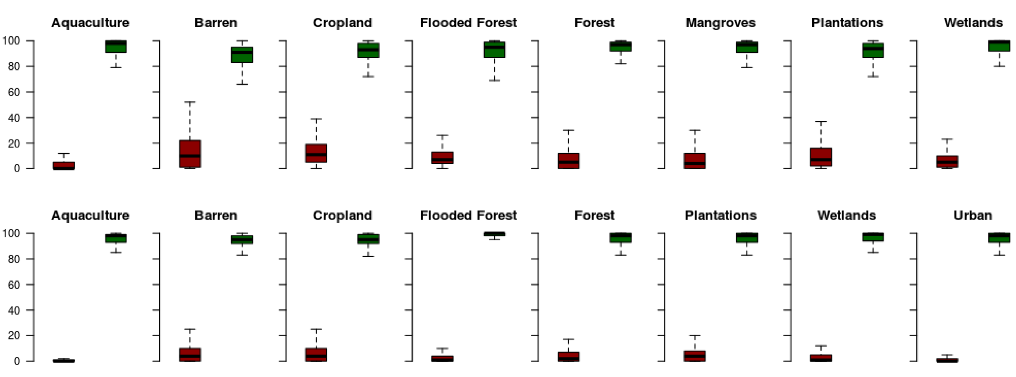
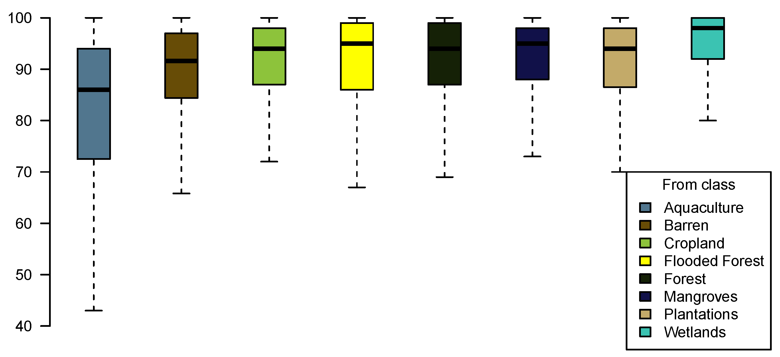
3.1. Spatial Change Dynamics

The 2018 change probability maps are shown in Figure 6 and Figure 7. The maps in Figure 6 show the probability of a pixel to change into any category. It can be seen that generally, higher probabilities were found for Plantations, Cropland and Forest, with lower probabilities for the other classes. Higher change probabilities for Cropland were found near the coast whereas, high probabilities for Forest change were found in Cambodia, Myanmar and Lao PDR.

Figure 7 shows the change probability for the ‘Generic to Specific’ category. This indicates the likelihood of a given pixel in any category to change into a specific class. It was found that anthropogenic land cover types including Plantations, Cropland, Urban, Aquaculture and Barren show higher probabilities. High change probabilities for Plantations are mostly focused around agricultural areas. The same case applies for Aquaculture, which shows high probabilities in agricultural areas in the delta, near the coast. High probabilities for Urban can be found near population centers. Higher change values are specifically notable in the red river delta in Northern Viet Nam. For Flooded forest and Wetlands we found high change probabilities around Tonle Sap lake, which is likely caused by the natural dynamics between these two classes.

Mapping both the ‘Specific to Generic’ and ‘Generic to Specific’ land cover change probabilities for each class revealed interesting dynamics, as it allowed a comparison of all the layers. For example, a visual inspection shows us that large areas in Cambodia have high probabilities in the ‘Specific to Generic’ Forest class and also high probabilities in the ‘Generic to specific’ Cropland class. At the same time, we can see high probabilities in the ‘Specific to Generic’ class for Cropland, whereas these areas show also a high probability in the ‘generic to specific’ class for Plantations. This could indicate that croplands have a greater likelihood to change into plantations. The ‘Generic to Specific’ Barren map (Figure 7) shows high probabilities for Croplands throughout the region whereas, the ‘Specific to Generic’ Cropland shows low probabilities for most of these areas. This is most likely caused by the fact that many croplands have a spectral signature of bare-land for part of the year. Changes from Cropland into any other class, including Barren, were not frequent in the training data whereas, changes from any other class to Barren carries a clear spectral signal of bare-land.

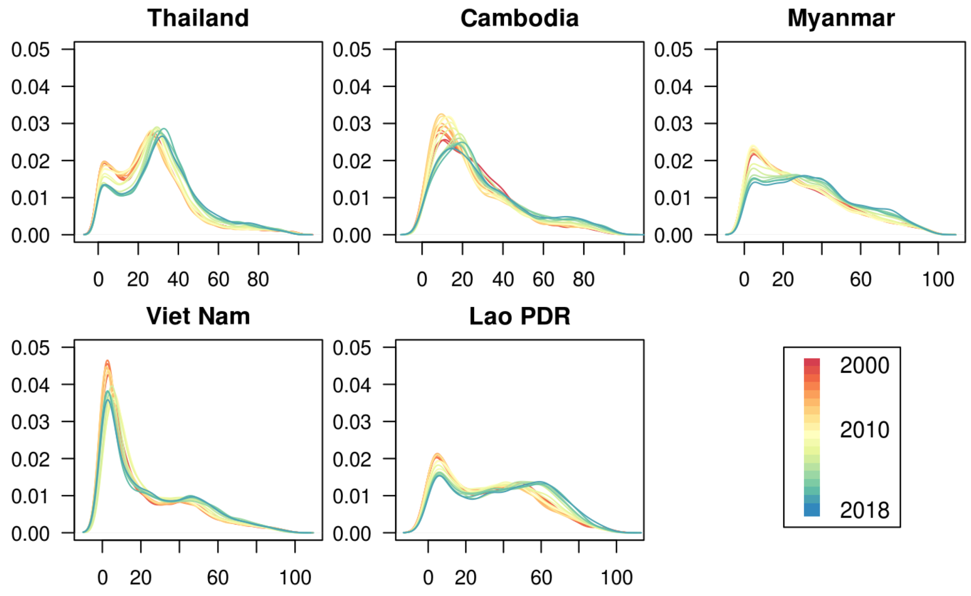
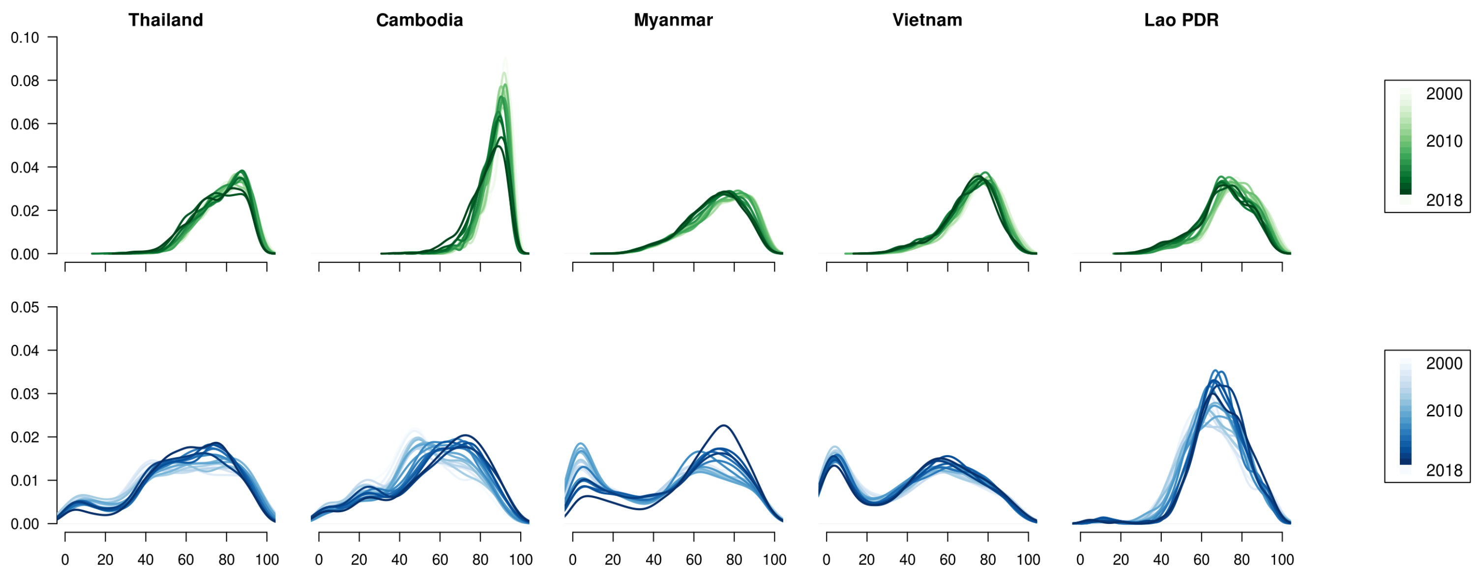
3.2. Temporal Change Dynamics

The time-series was used to investigate temporal forest dynamics. We sampled the yearly ‘Specific to Generic’ forest layer using 250,000 random points, while applying a temporal smoothing algorithm covering a year window. Figure 8 shows the probability density function for the ‘Specific to Generic’ forest data for the period 2000–2018 for each country. It is interesting to note that Thailand and Lao PDR, but also Viet Nam to some extent, show bi-modal distributions. The probability density functions of Myanmar and Cambodia show more similarity to log-normal distributions. All countries show a shift from low probabilities to higher probabilities. It is notable that the left modes decrease while the rights ones increase.

The ‘Specific to Generic’ Forest layer was then combined with the ‘Generic to Specific’ Cropland layer. We used the fifth percentile of Figure 4 and Figure 5 (62% and 72%) for the ‘Specific to Generic’ Forest and ‘Generic to Specific’ Cropland data, respectively, to mask the layers. Figure 9 shows the resulting distributions of the ‘Generic to Specific’ Cropland layer for all pixels with a high ‘Specific to Generic’ Forest probability (top: green color) as well as the ‘Specific to Generic’ Forest distributions with a high probability to change into Cropland (bottom: blue color). The different spectrum of colors indicate the different years.

It was found that the different combinations show different results. The probability density functions for all countries show a high probability in the ‘Generic to Specific’ Cropland category for pixels with a high probability in the ‘Specific to Generic’ category. This means that conversion to Cropland is very likely for all Forests that are under threat of deforestation. On the other hand, not all pixels that are likely to convert into Cropland are due to deforestation. This is evident in the bottom graphs of Figure 9 of Viet Nam, for example. The chart shows a bimodal distribution which indicates that except from Forest to Cropland conversion, there is another driver for cropland transitions. We found that change from Plantations is another important driver that shows a similar bimodal distribution for Viet Nam.

4. Discussion

We presented a methodology to map land cover change and its spatial and temporal dynamics. An interesting finding of this study is the bimodality of the probability density functions. In the context of a land cover type that needs to be preserved, it would mean that some areas are well protected, whilst other areas are under serious threat. For example, this could mean that either protection of that area is quite effective or, that the areas are very remote and therefore, more vulnerable. The shape and temporal dynamics of the probability functions provide important information for environmental protection, with a shift towards higher probabilities indicating a greater potential threat and a need for more effective policies.

In the study we used mostly yearly data as well as single time layers. One of the main limitations is the lack of yearly infrastructure and census data which is often difficult to obtain and has a coarse temporal resolution. However, it is important to include this data for this region considering the rapid economic developments over the last 20 years. Another limitation of the study is the lack of field validation. Figure 4 and Figure 5 show the probability distributions of an independent set of change pixels. The results provide reassurance that the model performs well in determining change probability. However, the independent sample was not verified by field observations. Field data for land cover change is often difficult to obtain but systems using higher resolution satellite imagery, such as Collect Earth, [53] offer exciting opportunities to collect new data. The work was conducted under the auspices of the Mekong River Commission (MRC), who intend to include locations with high change probabilities in their field data collection protocol. Future work could include further refinement of the model by incorporating field data for both training and validation purposes.

Conventional models to map land cover change include different components that determine land cover change pathways such as, the CLUE-S model which contains four components on land demand, suitability, policies and land use change rules [54]. These components are included implicitly in the covariates. For example terrain, water and rainfall indices provide information on suitability, whilst covariates derived from OpenStreetMap and WorldPop provide information on demand, and the layer on protected areas is important for policies. The change rules are set by machine learning, which assigns priorities to the different covariates based on historical change patterns, and then estimates potential future impacts. The method we presented is highly suitable scenario analysis. However, it should be noted that not all drivers are included in the model and that a high or low probability will not necessarily lead to land cover change in the future. Cloud-based geo-computation platforms enable on-the-fly exploration of the data and different scenarios as demonstrated by Poortinga et al. [55], Markert et al. [56]. For example, potential impacts of road construction can be studied by simply changing the covariate on distance to road and then running the model.

5. Conclusions

This study has developed a novel means to simulate and analyze land cover dynamics using EO, ground data and machine learning. Our machine learning-based approach is governed only by historical drivers of change, demonstrated by utilizing the land cover time-series maps generated by RLCMS for the Mekong region. We calculated the probability of the following classes: Aquaculture; Barren; Cropland; Flooded Forest; Forest; Mangroves; and Plantations, to change into any other ‘generic’ class. Additionally, we calculated the probability of any other ‘generic’ class to change into Aquaculture, Barren, Cropland, Flooded Forest, Forest, Plantations, Wetlands and Urban. It was found that historical change pixels all exhibit mean change probabilities greater than 80%, along with lower quantiles, except one, being greater than 70%. The highest change probabilities in the ‘Specific to Generic’ category were the Cropland and Forest classes. Whereas, for the ‘Generic to Specific’ category, the classes with the highest change probabilities were Plantations, Cropland, Urban and Aquaculture. We sampled layers based on administrative boundaries and showed that the associated probability distributions provide important information on temporal change dynamics. This research successfully illustrates that machine learning, combined with single time and time-series data layers including EO, can be used to identify potential land cover change hotspots and land cover change trajectories—information that is important for sustainable decision-making regarding land-use planning and management. Whilst the focus for this study was the Mekong region, our approach in principle can be up-scaled and applied on a planetary scale, beneficial for a wide range of stakeholders from land planners to policy makers.

References

1. Houghton, R.A.; House, J.; Pongratz, J.; Van Der Werf, G.; DeFries, R.; Hansen, M.; Quéré, C.L.; Ramankutty, N. Carbon emissions from land use and land-cover change. Biogeosciences 2012, 9, 5125–5142. [Google Scholar] [CrossRef] [Green Version]
2. Poortinga, A.; Tenneson, K.; Shapiro, A.; Nquyen, Q.; San Aung, K.; Chishtie, F.; Saah, D. Mapping plantations in Myanmar by fusing landsat-8, sentinel-2 and sentinel-1 data along with systematic error quantification. Remote Sens. 2019, 11, 831. [Google Scholar] [CrossRef] [Green Version]
3. Poortinga, A.; Nguyen, Q.; Tenneson, K.; Troy, A.; Bhandari, B.; Ellenburg, W.L.; Aekakkararungroj, A.; Ha, L.T.; Pham, H.; Nguyen, G.V.; et al. Linking earth observations for assessing the food security situation in Vietnam: A landscape approach. Front. Environ. Sci. 2019, 7, 186. [Google Scholar] [CrossRef] [Green Version]
4. Bewket, W. Land cover dynamics since the 1950s in Chemoga watershed, Blue Nile basin, Ethiopia. Mountain Res. Dev. 2002, 22, 263–270. [Google Scholar] [CrossRef] [Green Version]
5. Stürck, J.; Poortinga, A.; Verburg, P.H. Mapping ecosystem services: The supply and demand of flood regulation services in Europe. Ecol. Indicat. 2014, 38, 198–211. [Google Scholar] [CrossRef]
6. Poortinga, A.; Bastiaanssen, W.; Simons, G.; Saah, D.; Senay, G.; Fenn, M.; Bean, B.; Kadyszewski, J. A self-calibrating runoff and streamflow remote sensing model for ungauged basins using open-access earth observation data. Remote Sens. 2017, 9, 86. [Google Scholar] [CrossRef] [Green Version]
7. Trisurat, Y.; Alkemade, R.; Verburg, P.H. Projecting land-use change and its consequences for biodiversity in Northern Thailand. Environ. Manag. 2010, 45, 626–639. [Google Scholar] [CrossRef] [PubMed] [Green Version]
8. Tizora, P.; le Roux, A.; Mans, G.; Cooper, A.K. Adapting the Dyna-CLUE model for simulating land use and land cover change in the Western Cape Province. S. Afr. J. Geomat. 2018, 7, 190–203. [Google Scholar] [CrossRef] [Green Version]
9. Verburg, P.H. Simulating feedbacks in land use and land cover change models. Landsc. Ecol. 2006, 21, 1171–1183. [Google Scholar] [CrossRef]
10. Verburg, P.H.; Schot, P.P.; Dijst, M.J.; Veldkamp, A. Land use change modelling: Current practice and research priorities. GeoJournal 2004, 61, 309–324. [Google Scholar] [CrossRef]
11. Schaldach, R.; Priess, J.A. Integrated Models of the Land System: A Review of Modelling Approaches on the Regional to Global Scale. Living Rev. Landsc. Res. 2008, 2. [Google Scholar] [CrossRef] [Green Version]
12. Matthews, R.B.; Gilbert, N.G.; Roach, A.; Polhill, J.G.; Gotts, N.M. Agent-based land-use models: A review of applications. Landsc. Ecol. 2007, 22, 1447–1459. [Google Scholar] [CrossRef] [Green Version]
13. Saah, D.; Tenneson, K.; Poortinga, A.; Nguyen, Q.; Chishtie, F.; San Aung, K.; Markert, K.N.; Clinton, N.; Anderson, E.R.; Cutter, P.; et al. Primitives as building blocks for constructing land cover maps. Int. J. Appl. Earth Obs. Geoinf. 2020, 85, 101979. [Google Scholar] [CrossRef]
14. Saah, D.; Tenneson, K.; Matin, M.; Uddin, K.; Cutter, P.; Poortinga, A.; Ngyuen, Q.H.; Patterson, M.; Johnson, G.; Markert, K.; et al. Land cover mapping in data scarce environments: Challenges and opportunities. Front. Environ. Sci. 2019, 7, 150. [Google Scholar] [CrossRef] [Green Version]
15. Simons, G.; Poortinga, A.; Bastiaanssen, W.G.; Saah, D.; Troy, D.; Hunink, J.; Klerk, M.d.; Rutten, M.; Cutter, P.; Rebelo, L.M.; et al. On Spatially Distributed Hydrological Ecosystem Services: Bridging the Quantitative Information Gap using Remote Sensing and Hydrological Models; CGIAR: Wageningen, The Netherlands, 2017. [Google Scholar]
16. Phongsapan, K.; Chishtie, F.; Poortinga, A.; Bhandari, B.; Meechaiya, C.; Kunlamai, T.; Aung, K.S.; Saah, D.; Anderson, E.; Markert, K.; et al. Operational flood risk index mapping for disaster risk reduction using Earth Observations and cloud computing technologies: A case study on Myanmar. Front. Environ. Sci. 2019, 7, 191. [Google Scholar] [CrossRef] [Green Version]
17. Pal, M. Random forest classifier for remote sensing classification. Int. J. Remote Sens. 2005, 26, 217–222. [Google Scholar] [CrossRef]
18. Fernández-Delgado, M.; Cernadas, E.; Barro, S.; Amorim, D. Do we need hundreds of classifiers to solve real world classification problems? J. Mach. Learn. Res. 2014, 15, 3133–3181. [Google Scholar]
19. Zhu, Z.; Woodcock, C.E. Object-based cloud and cloud shadow detection in Landsat imagery. Remote Sens. Environ. 2012, 118, 83–94. [Google Scholar] [CrossRef]
20. Young, N.E.; Anderson, R.S.; Chignell, S.M.; Vorster, A.G.; Lawrence, R.; Evangelista, P.H. A survival guide to Landsat preprocessing. Ecology 2017, 98, 920–932. [Google Scholar] [CrossRef] [Green Version]
21. Chastain, R.; Housman, I.; Goldstein, J.; Finco, M. Empirical cross sensor comparison of Sentinel-2A and 2B MSI, Landsat-8 OLI, and Landsat-7 ETM+ top of atmosphere spectral characteristics over the conterminous United States. Remote Sens. Environ. 2019, 221, 274–285. [Google Scholar] [CrossRef]
22. Roy, D.P.; Ju, J.; Lewis, P.; Schaaf, C.; Gao, F.; Hansen, M.; Lindquist, E. Multi-temporal MODIS–Landsat data fusion for relative radiometric normalization, gap filling, and prediction of Landsat data. Remote Sens. Environ. 2008, 112, 3112–3130. [Google Scholar] [CrossRef]
23. Gao, F.; He, T.; Masek, J.G.; Shuai, Y.; Schaaf, C.B.; Wang, Z. Angular effects and correction for medium resolution sensors to support crop monitoring. IEEE J. Sel. Top. Appl. Earth Obs. Remote Sens. 2014, 7, 4480–4489. [Google Scholar] [CrossRef]
24. Roy, D.P.; Li, J.; Zhang, H.K.; Yan, L.; Huang, H.; Li, Z. Examination of Sentinel-2A multi-spectral instrument (MSI) reflectance anisotropy and the suitability of a general method to normalize MSI reflectance to nadir BRDF adjusted reflectance. Remote Sens. Environ. 2017, 199, 25–38. [Google Scholar] [CrossRef]
25. Lucht, W.; Schaaf, C.B.; Strahler, A.H. An algorithm for the retrieval of albedo from space using semiempirical BRDF models. IEEE Trans. Geosci. Remote Sens. 2000, 38, 977–998. [Google Scholar] [CrossRef] [Green Version]
26. Roy, D.P.; Zhang, H.; Ju, J.; Gomez-Dans, J.L.; Lewis, P.E.; Schaaf, C.; Sun, Q.; Li, J.; Huang, H.; Kovalskyy, V. A general method to normalize Landsat reflectance data to nadir BRDF adjusted reflectance. Remote Sens. Environ. 2016, 176, 255–271. [Google Scholar] [CrossRef] [Green Version]
27. Justice, C.O.; Wharton, S.W.; Holben, B. Application of digital terrain data to quantify and reduce the topographic effect on Landsat data. Int. J. Remote Sens. 1981, 2, 213–230. [Google Scholar] [CrossRef] [Green Version]
28. Smith, J.; Lin, T.L.; Ranson, K. The Lambertian assumption and Landsat data. Photogram. Eng. Remote Sens. 1980, 46, 1183–1189. [Google Scholar]
29. Teillet, P.; Guindon, B.; Goodenough, D. On the slope-aspect correction of multispectral scanner data. Can. J. Remote Sens. 1982, 8, 84–106. [Google Scholar] [CrossRef] [Green Version]
30. Soenen, S.A.; Peddle, D.R.; Coburn, C.A. SCS+ C: A modified sun-canopy-sensor topographic correction in forested terrain. IEEE Trans. Geosci. Remote Sens. 2005, 43, 2148–2159. [Google Scholar] [CrossRef]
31. Flood, N. Seasonal composite Landsat TM/ETM+ images using the medoid (a multi-dimensional median). Remote Sens. 2013, 5, 6481–6500. [Google Scholar] [CrossRef] [Green Version]
32. Vermote, E.; Vermeulen, A. Atmospheric correction algorithm: Spectral reflectances (MOD09). ATBD Vers. 1999, 4, 1–107. [Google Scholar]
33. Jiang, Z.; Huete, A.R.; Didan, K.; Miura, T. Development of a two-band enhanced vegetation index without a blue band. Remote Sens. Environ. 2008, 112, 3833–3845. [Google Scholar] [CrossRef]
34. Xu, H. A new index for delineating built-up land features in satellite imagery. Int. J. Remote Sens. 2008, 29, 4269–4276. [Google Scholar] [CrossRef]
35. McFeeters, S.K. The use of the Normalized Difference Water Index (NDWI) in the delineation of open water features. Int. J. Remote Sens. 1996, 17, 1425–1432. [Google Scholar] [CrossRef]
36. Salomonson, V.V.; Appel, I. Estimating fractional snow cover from MODIS using the normalized difference snow index. Remote Sens. Environ. 2004, 89, 351–360. [Google Scholar] [CrossRef]
37. Rouse, J., Jr.; Haas, R.; Schell, J.; Deering, D. Monitoring Vegetation Systems in the Great Plains With ERTS; NASA: Washington, DC, USA, 1974. [Google Scholar]
38. Key, C.H.; Benson, N.C. The Normalized Burn Ratio (NBR): A Landsat TM Radiometric Measure Of Burn Severity; United States Geological Survey, Northern Rocky Mountain Science Center: Bozeman, MT, USA, 1999. [Google Scholar]
39. Crist, E.P.; Cicone, R.C. A physically-based transformation of Thematic Mapper data—The TM Tasseled Cap. IEEE Trans. Geosci. Remote Sens. 1984, 256–263. [Google Scholar] [CrossRef]
40. Contributors, O. Planet Dump. 2017. Available online: https://www.openstreetmap.org (accessed on 4 May 2020).
41. Farr, T.G.; Rosen, P.A.; Caro, E.; Crippen, R.; Duren, R.; Hensley, S.; Kobrick, M.; Paller, M.; Rodriguez, E.; Roth, L.; et al. The shuttle radar topography mission. Rev. Geophys. 2007, 45. [Google Scholar] [CrossRef] [Green Version]
42. Potapov, P.; Tyukavina, A.; Turubanova, S.; Talero, Y.; Hernandez-Serna, A.; Hansen, M.; Saah, D.; Tenneson, K.; Poortinga, A.; Aekakkararungroj, A.; et al. Annual continuous fields of woody vegetation structure in the Lower Mekong region from 2000–2017 Landsat time-series. Remote Sens. Environ. 2019, 232, 111278. [Google Scholar] [CrossRef]
43. Tatem, A.J. WorldPop, open data for spatial demography. Sci. Data 2017, 4. [Google Scholar] [CrossRef]
44. Funk, C.; Peterson, P.; Landsfeld, M.; Pedreros, D.; Verdin, J.; Shukla, S.; Husak, G.; Rowland, J.; Harrison, L.; Hoell, A.; et al. The climate hazards infrared precipitation with stations—A new environmental record for monitoring extremes. Sci. Data 2015, 2, 150066. [Google Scholar] [CrossRef] [Green Version]
45. Olson, D.M.; Dinerstein, E.; Wikramanayake, E.D.; Burgess, N.D.; Powell, G.V.; Underwood, E.C.; D’amico, J.A.; Itoua, I.; Strand, H.E.; Morrison, J.C.; et al. Terrestrial Ecoregions of the World: A New Map of Life on EarthA new global map of terrestrial ecoregions provides an innovative tool for conserving biodiversity. BioScience 2001, 51, 933–938. [Google Scholar] [CrossRef]
46. Pekel, J.F.; Cottam, A.; Gorelick, N.; Belward, A.S. High-resolution mapping of global surface water and its long-term changes. Nature 2016, 540, 418. [Google Scholar] [CrossRef] [PubMed]
47. Stevens, F.R.; Gaughan, A.E.; Linard, C.; Tatem, A.J. Disaggregating census data for population mapping using random forests with remotely-sensed and ancillary data. PLoS ONE 2015, 10, e0107042. [Google Scholar] [CrossRef] [PubMed] [Green Version]
48. Hansen, M.C.; Egorov, A.; Roy, D.P.; Potapov, P.; Ju, J.; Turubanova, S.; Kommareddy, I.; Loveland, T.R. Continuous fields of land cover for the conterminous United States using Landsat data: First results from the Web-Enabled Landsat Data (WELD) project. Remote Sens. Lett. 2011, 2, 279–288. [Google Scholar] [CrossRef]
49. Hansen, M.C.; Potapov, P.V.; Goetz, S.J.; Turubanova, S.; Tyukavina, A.; Krylov, A.; Kommareddy, A.; Egorov, A. Mapping tree height distributions in Sub-Saharan Africa using Landsat 7 and 8 data. Remote Sens. Environ. 2016, 185, 221–232. [Google Scholar] [CrossRef] [Green Version]
50. Trimble, G.R., Jr.; Weitzman, S. Site index studies of upland oaks in the northern Appalachians. Forest Sci. 1956, 2, 162–173. [Google Scholar]
51. Beers, T.W.; Dress, P.E.; Wensel, L.C. Notes and observations: Aspect transformation in site productivity research. J. For. 1966, 64, 691–692. [Google Scholar]
52. Jeswani, R.; Kulshrestha, A.; Gupta, P.K.; Srivastav, S. Evaluation of the consistency of DMSP-OLS and SNPP-VIIRS Night-time Light Datasets. Master’s Thesis, University of Twente, Enschede, The Netherland, 2017. [Google Scholar]
53. Saah, D.; Johnson, G.; Ashmall, B.; Tondapu, G.; Tenneson, K.; Patterson, M.; Poortinga, A.; Markert, K.; Quyen, N.H.; San Aung, K.; et al. Collect Earth: An online tool for systematic reference data collection in land cover and use applications. Environ. Model. Softw. 2019. [Google Scholar] [CrossRef]
54. Xu, L.; Li, Z.; Song, H.; Yin, H. Land-use planning for urban sprawl based on the clue-s model: A Case study of Guangzhou, China. Entropy 2013, 15, 3490–3506. [Google Scholar] [CrossRef]
55. Poortinga, A.; Clinton, N.; Saah, D.; Cutter, P.; Chishtie, F.; Markert, K.N.; Anderson, E.R.; Troy, A.; Fenn, M.; Tran, L.H.; et al. An Operational Before-After-Control-Impact (BACI) Designed Platform for Vegetation Monitoring at Planetary Scale. Remote Sens. 2018, 10, 760. [Google Scholar] [CrossRef] [Green Version]
56. Markert, K.; Schmidt, C.; Griffin, R.; Flores, A.; Poortinga, A.; Saah, D.; Muench, R.; Clinton, N.; Chishtie, F.; Kityuttachai, K.; et al. Historical and operational monitoring of surface sediments in the lower mekong basin using landsat and google earth engine cloud computing. Remote Sens. 2018, 10, 909. [Google Scholar] [CrossRef] [Green Version]
Figure 1. The Mekong study area includes Cambodia, Lao People’s Democratic Republic, Myanmar, Thailand, and Viet Nam.
Remotesensing 12 01472 g001
Figure 2. Overview of training (top) and validation (bottom) samples used in the study. Images on the left show data points in the ‘specific to generic’ category, images on the right ‘generic to specific’. Different colors represent the different classes.
Remotesensing 12 01472 g002
Figure 3. Distributions of the training data samples for ‘Specific to Generic’ (top row) and ‘Generic to Specific’ (bottom row). The red boxes show change probabilities of pixels that did not change, the green boxes for the change pixels.
Remotesensing 12 01472 g003
Figure 4. Distributions of validation change pixels in the ‘Specific to Generic’ category.
Remotesensing 12 01472 g004
Figure 5. Distributions of validation change pixels in the ‘Generic to Specific’ category.
Remotesensing 12 01472 g005
Figure 6. Probability change maps for ‘Specific to Generic’ category for the different land cover types. The maps show the probability of a pixel to change into any other category for the year 2018.
Remotesensing 12 01472 g006
Figure 7. Probability change maps for ‘Generic to specific’ category for the different land cover types. The maps show the probability of a pixel to change into that specific category for the year 2018.
Remotesensing 12 01472 g007
Figure 8. Densities of probability of changes for the ‘Specific to Generic’ forest data per country for the period 2000–2018.
Remotesensing 12 01472 g008
Figure 9. Probability density functions for anthropogenic change. The green charts show the ‘Generic to Specific’ cropland distributions per country, filtered using the ‘Specific to Generic’ Forest data with a threshold of 62%. The blue charts show the ‘Specific to Generic’ Forest distribution of the ‘Generic to Specific’ Cropland layers with a threshold value of 72%.
Remotesensing 12 01472 g009