Article

Monitoring 10-m LST from the Combination MODIS/Sentinel-2, Validation in a High Contrast Semi-Arid Agroecosystem

by
Juan M. Sánchez
1,*,
Joan M. Galve
1,
José González-Piqueras
1,
Ramón López-Urrea
2,
Raquel Niclòs
3 and
Alfonso Calera
1
1
Regional Development Institute, University of Castilla-La Mancha, Campus Universitario s/n, 02071 Albacete, Spain
2
Instituto Técnico Agronómico Provincial de Albacete and FUNDESCAM, Parque Empresarial Campollano, 2ª Avda. N°61, 02007 Albacete, Spain
3
Earth Physics and Thermodynamics Department, University of Valencia, C/ Dr. Moliner 50, 46100 Burjassot, Spain
*
Author to whom correspondence should be addressed.
Remote Sens. 2020, 12(9), 1453; https://doi.org/10.3390/rs12091453
Submission received: 25 March 2020 / Revised: 24 April 2020 / Accepted: 1 May 2020 / Published: 4 May 2020
(This article belongs to the Special Issue Remote Sensing Monitoring of Land Surface Temperature (LST))

Abstract

:
Downscaling techniques offer a solution to the lack of high-resolution satellite Thermal InfraRed (TIR) data and can bridge the gap until operational TIR missions accomplishing spatio-temporal requirements are available. These techniques are generally based on the Visible Near InfraRed (VNIR)-TIR variable relations at a coarse spatial resolution, and the assumption that the relationship between spectral bands is independent of the spatial resolution. In this work, we adopted a previous downscaling method and introduced some adjustments to the original formulation to improve the model performance. Maps of Land Surface Temperature (LST) with 10-m spatial resolution were obtained as output from the combination of MODIS/Sentinel-2 images. An experiment was conducted in an agricultural area located in the Barrax test site, Spain (39°03′35″ N, 2°06′ W), for the summer of 2018. Ground measurements of LST transects collocated with the MODIS overpasses were used for a robust local validation of the downscaling approach. Data from 6 different dates were available, covering a variety of croplands and surface conditions, with LST values ranging 300–325 K. Differences within ±4.0 K were observed between measured and modeled temperatures, with an average estimation error of ±2.2 K and a systematic deviation of 0.2 K for the full ground dataset. A further cross-validation of the disaggregated 10-m LST products was conducted using an additional set of Landsat-7/ETM+ images. A similar uncertainty of ±2.0 K was obtained as an average. These results are encouraging for the adaptation of this methodology to the tandem Sentinel-3/Sentinel-2, and are promising since the 10-m pixel size, together with the 3–5 days revisit frequency of Sentinel-2 satellites can fulfill the LST input requirements of the surface energy balance methods for a variety of hydrological, climatological or agricultural applications. However, certain limitations to capture the variability of extreme LST, or in recently sprinkler irrigated fields, claim the necessity to explore the implementation of soil moisture or vegetation indices sensitive to soil water content as inputs in the downscaling approach. The ground LST dataset introduced in this paper will be of great value for further refinements and assessments.

1. Introduction

Time series of fine spatial and temporal resolution Thermal Infrared Images (TIR) are essential in a variety of agricultural applications, water resources management or irrigation scheduling, based on surface energy balance modeling [1,2,3,4]. However, spatio-temporal resolution of the operational TIR satellite sensors results are insufficient for some applications and services, including agriculture. The importance of high-resolution TIR images is being claimed [5,6,7,8,9]. The limitation in the TIR domain remains, since the revisit time for high spatial resolution TIR sensors is typically poor, while the spatial resolution for those with a high revisit frequency is too coarse. In practice, the spatial resolution requirements of satellite-derived surface temperature for agricultural applications are <50 m to face certain physical limitations related to the sensor’s point spread function in TIR observations [2,10,11]. As for the temporal resolution, daily TIR observations are desired, although this requirement could be relaxed to 3 days as a minimum threshold [7,11].
The Copernicus conceptual mission LSTM [12] could complement other planned high-resolution TIR missions (e.g., the JPL-NASA Landsat 9-10 or the Indian-French TRISHNA mission [13]) and fulfill the spatio-temporal requirements stated above. In the meantime, downscaling methods are contributing to filling this gap by downscaling the TIR coarse resolution to finer resolutions [3,14,15,16,17]. Several techniques have been proposed in the literature to enhance the spatial resolution of the TIR domain over vegetated areas by linking TIR and reflectance information in the Visible Near Infrared (VNIR) [18,19,20,21]. These techniques are generally based on the assumption that there exists a relation between the vegetation cover and the LST. According to these approaches, a relation between the TIR and VNIR bands is first obtained at coarse spatial resolution, and then applied at the finer resolution of the VNIR bands, assuming that this relation is scale invariant.
The Normalized Difference Vegetation Index (NDVI) or the Fractional Vegetation Cover (FVC) are the most commonly used inputs in sharpening techniques, although some studies have recently explored the possibility of implementing other combinations of reflectance values that can better characterize the surface response [17,22,23]. There are also some efforts attempting to integrate soil moisture delineated vegetation indices [24], and even radar-derived soil moisture [25] in the formulations of the LST downscaling.
For years, the Moderate Resolution Imaging Spectroradiometer (MODIS) or the Advanced Along-Track Scanning Radiometer (AATSR) were combined with Landsat or Advanced Spaceborne Thermal Emission and Reflection Radiometer (ASTER) imagery to downscale LST from 1000 m × 1000 m to ~1 ha (10,000 m2) scale. Higher resolution VNIR sensors, such as Formosat or the Satellite pour l´Observation de la Terre (SPOT), have been also used to improve the disaggregated LST pixel size [10,26].
The synergistic use of Copernicus Sentinel-2 (S2) and Sentinel-3 (S3) imagery could offer the desired solution of high spatial and temporal resolution [8,26,27]. Although no TIR information is provided, the Sentinel-2A and -2B tandem offers a 3–5-day repeat cycle, and a 10–20 m spatial resolution in the VNIR bands. Revisit time for S3 reduces to 1–2 days, with a spatial resolution of 1000 m for their thermal channels. The relationship between TIR and VNIR bands could be extracted from S3 and then applied to S2 VNIR data. Sobrino et al. [27] explored the conceptual combination of the MultiSpectral Instrument (MSI), on board the Sentinel-2, and the Ocean and Land Color Instrument/Sea and Land Surface Temperature Radiometer (OLCI/SLSTR), on board the Sentinel-3, to show an improvement in LST products derived from AATSR at that time, before the Sentinel-3 data were available. High spatial resolution data from S2 was used to improve the characterization of the sub-pixel heterogeneity through a better parameterization of surface emissivity, although no downscaling was applied by these authors. A machine learning algorithm was proposed by Guzinski and Nieto [8] to sharpen low-resolution TIR observations from S3 using high-resolution VNIR S2 imagery. Huryna et al. [28] applied the methodology introduced by Agam et al. [19] to the combination of S3–S2 imagery. However, the methodology was tested using Terra/MODIS or Landsat observations in both works, due to the lack of high-resolution TIR data to use for cross-validation.
Despite the extraordinary growth of downscaling studies in the past decade, the assessment of the thermal sharpening techniques has been traditionally conducted by cross-validation with derived LST products at original Landsat or ASTER TIR spatial resolutions, 60–100 m and 90 m, respectively [1,8,17,21,28]. Comprehensive ground validations of disaggregated LST are quite scarce, due to the lack of robust datasets covering high contrast heterogeneous areas.
This paper continues the work initiated by Bisquert et al. [1]. These authors tested the application of different downscaling techniques in an experimental site in Barrax (Albacete, Spain) from the combination MODIS-Landsat to provide LST at fine spatial and temporal resolutions, to fulfill the requirements in the estimation of surface energy fluxes and evapotranspiration in the agricultural areas of semi-arid regions, where small land holdings dominate. Bisquert et al. [1] analyzed both classical methods based on the VNIR-LST regression, as well as more advanced approaches based on Neural Networks (NN) or Data Mining (DM). Linear, quadratic and exponential relationships, proposed in the literature, were tested and results were compared to those obtained by applying NN and regression trees in a DM approach using reflectance values from all the spectral bands available. These authors observed that NN and DM, as well as the nonlinear regression tested, have the risk of overfitting, being very sensitive to noise in the samples. They concluded that the simpler NDVI-LST linear regression led to the better results in this case. Bisquert et al. [1] explored the technique results for the different land covers in the Barrax area, and found the largest uncertainties for irrigated croplands, especially in summer when cover heterogeneity and irrigation effects are stressed. As a follow-up, Bisquert et al. [26] extracted disaggregated LST maps at a 10-m spatial resolution for the first time, using high-resolution SPOT-5 images in the framework of the Spot-5 Take 5 project. Results shown in [26] were encouraging for the further application of the model to operational S2 images.
In this context, the objective of this paper is to revise and adapt the downscaling technique to the combination MODIS-S2 to derive operational LST maps with a spatial resolution of 10 m. Some adjustments to the original formulation of the approach were introduced to reduce the model uncertainty by adding an additional image-based parametrization of the residual as a function of the VNIR response. Ground LST data from an experimental campaign carried out in the summer of 2018 were used for the model evaluation. The variety of croplands and the contrast in the surface conditions during the experiment in the selected area allowed a comprehensive analysis of the performance of the downscaling technique, not achieved before. Strengths and limitations of the models were discussed, and also some guidelines for the optimal use of this technique with Sentinel-3 and Sentinel-2 imagery are given.
This paper is structured as follows. Section 2 describes the study site, the field measurements and the satellite imagery used, as well as the downscaling methodology. Results of the ground validation and distributed assessment are shown in Section 3. Interpretation of the results and comparison with previous studies comprise Section 4. Finally, Section 5 summarizes the main conclusions of this work.

2. Materials and Methods

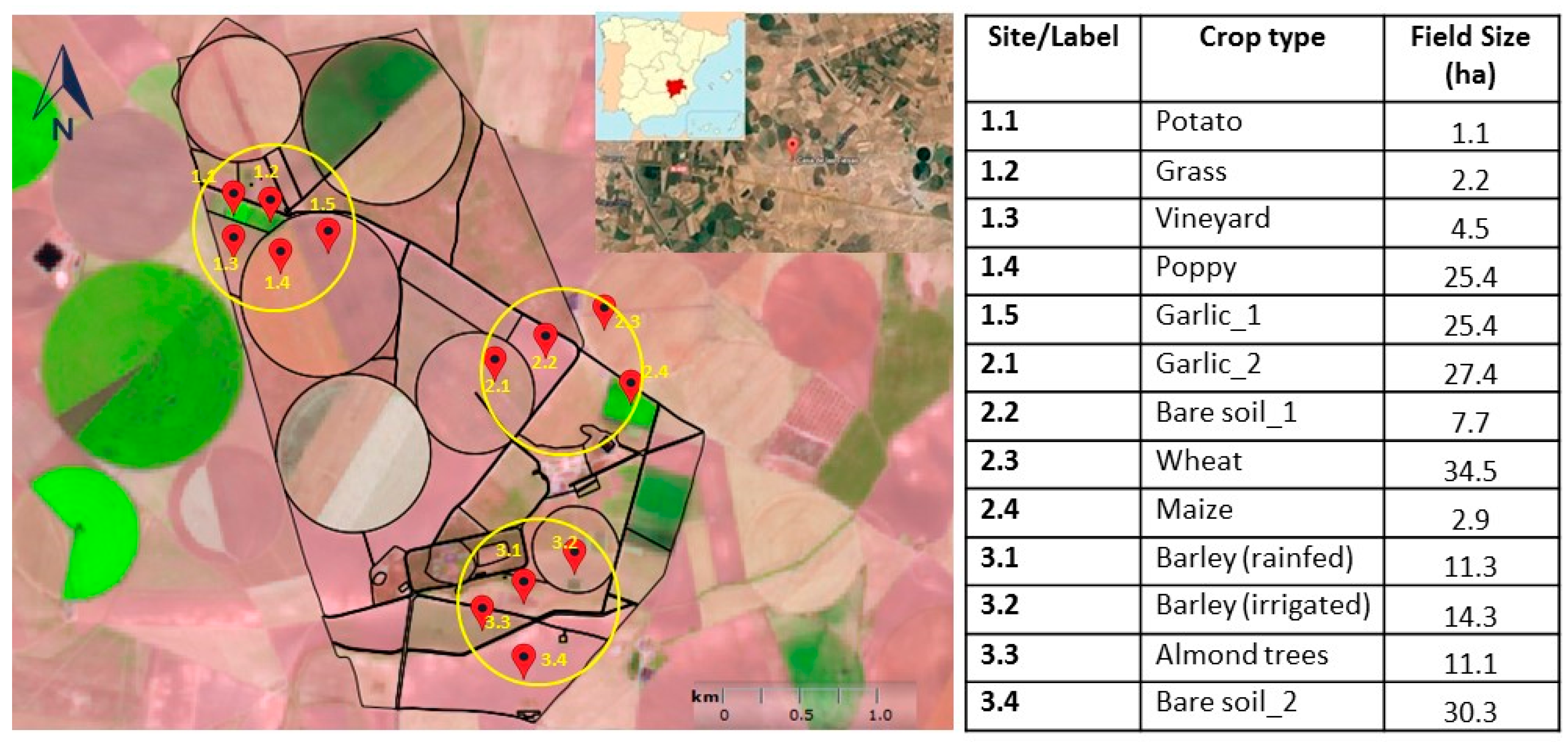
2.1. Study Site and Measurements

This work was conducted in the semi-arid area of Barrax, southeast Spain (39°03′ N, 2°06′ W). This is a very flat area with an average altitude of 700 m a.s.l, close to Albacete (Figure 1), traditionally used by ESA (European Space Agency) as a test site in different international campaigns [29,30,31]. Irrigated and rainfed crops combine in this agroecosystem, with field size ranging from small terrains below 1 ha to large pivots over 50 ha (Figure 1). This large variety makes Barrax a perfect target to assess the performance of a downscaling technique and explore its strengths and weaknesses.
Ground measurements of LST (LSTg) were registered in “Las Tiesas” experimental farm during the summer of 2018, concurrent with EOS-Terra/MODIS overpasses, and covering a total of 10 different crops in 13 independent fields (Figure 1). The temperatures were measured using four hand-held infrared radiometers (IRTs) Apogee MI-210. These radiometers have a broad thermal band (8–14 µm), with a 22° field of view and an accuracy of ±0.2 K, according to the manufacturer (Apogee Instruments, Inc.). In fact, the similar Apogee SI-121 radiometers (same radiometer, but with a field of view of 18° and without datalogger) were calibrated against a National Institute of Standards and Technology (NIST) blackbody, during a comparison of TIR radiometers carried out in Miami by the Committee on Earth Observation Satellites (CEOS), and the accuracy was established at 0.2 K [32]. Special care was taken with the ground measurements in the sparse crops (vineyard and almond orchards), by averaging soil and canopy component temperatures to obtain representative values of the target LST. The radiometers were manually carried back and forth along transects on the fields pointing at nadir view, at a height of 1.5–2 m above the ground surface. Temperatures were registered at a rate of 5–10 measurements/min, in transect distances of 30–50 m/min, and then covering several hectares with each IRT. The 10-min averages centered at the satellite overpass time were considered. Radiometric temperatures were corrected from atmospheric and emissivity effects [33]. Downwelling sky radiance was measured with each radiometer and emissivity data were obtained through the Temperature-Emissivity Separation (TES) procedure [34,35] from in situ thermal radiance measurements using a multispectral radiometer CIMEL Electronique CE 312-2 [36].

2.2. Satellite Images

Terra/MODIS images with near nadir observations of the study site (field of view <25°) were selected to minimize the bowtie effect [37]. Six different dates were used for this work (Table 1). MODIS VNIR and TIR data were extracted from the MOD09GQ, and MOD11_L2 products, respectively, downloaded from the NASA Earthdata Search tool. MOD09GQ offers surface Red and NIR reflectivity values at a 250 m spatial resolution. MOD11_L2 product provides LST, atmospherically corrected with a split-window algorithm, at a 1000 m spatial resolution [38].
Sentinel-2A and Sentinel-2B images concurrent or within ±1-day timing difference with MODIS were used (see dates in Table 1). S2 Level-2A products were downloaded from the Copernicus Open Access Hub, and they contain 10-m surface reflectance values. Bands 4 and 8 were used to compose the Normalized Difference Vegetation Index (NDVI). Figure 2 shows an example of the spatial distribution of the NDVI over the study site. Note the wide range in NDVI values available in the area during the experiment. Plot in Figure 3 shows the NDVI values for the different crop fields in the selected dates.
Landsat-7/ETM+ overpasses were also available for 3 of the selected dates (9, 16 and 25 July). Although ETM+ TIR band has a resolution of 60 m, a cubic convolution resampling to 30 m is applied for user distribution. Thus, these images, with a 30-m spatial resolution, were used as a reference for an extended validation of the disaggregated LST. For the VNIR bands the Landsat Surface Reflectance (CDR) product was used, whereas the original TIR data in band 6 were corrected from atmospheric and emissivity effects following the method proposed by Galve et al. [39].

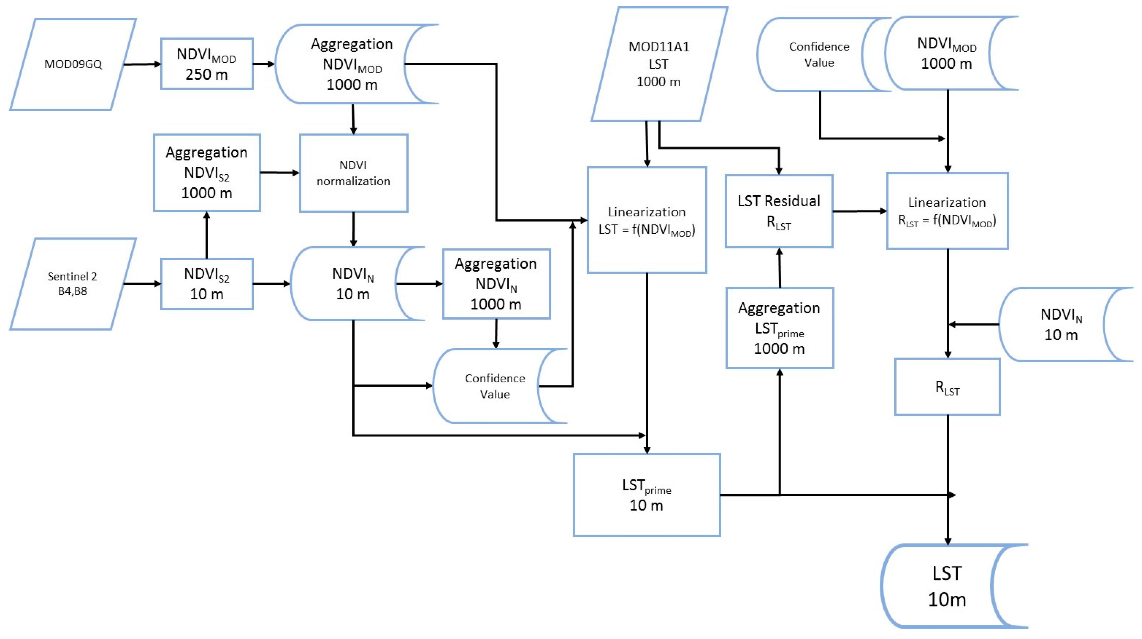
2.3. Downscaling Approach

Bisquert et al. [1] tested different downscaling methods with pairs of Landsat/MODIS images in this Barrax area. A modification of the sharpening method presented by Agam et al. [19] showed the best results. This method is based on the linear relationship established between NDVI and LST at the MODIS 1000 m resolution (NDVIMOD and LSTMOD, respectively). The approach outlined by Bisquert et al. [1] has been revised and adapted to the combination MODIS-S2 and used in this work as a basis to derive 10-m LST maps.
The flowchart in Figure 4 shows the main steps and calculations of this downscaling algorithm that can be summarized as follows:
  • The aggregation of the VNIR bands was carried out by averaging the reflectance values in the red and NIR bands of the 10-m S2 pixels, and 250-m MODIS pixels within an equivalent 1000 m MODIS pixel;
  • NDVI values were calculated from both S2 (NDVIS2) and MODIS (NDVIMOD) VNIR data at 1000 m resolution;
  • Differences between S2 and MODIS VNIR data due to spectral resolution, atmospheric correction, viewing angle or pixel footprint were corrected through a normalization extracted from the 1000 m NDVI, then applied to 10-m S2 NDVI (NDVIN);
  • The 1000 m coarse spatial resolution required a previous selection of “pure” pixels for the NDVI-LST adjustment. This selection was based on a confidence value calculated from the comparison between NDVIMOD and aggregated NDVIN. This confidence value was computed as the ratio between the standard deviation from the 4 × 4 pixels belonging to each 1000 m pixel, and its mean value, as suggested by [18]. Pixels with confidence values within the lowest quartile were selected in this step;
  • A linear regression was established between NDVIMOD and LSTMOD at 1000 m, using data from those “pure” pixels, and then applied to the NDVIN values to obtain a prime estimate of 10-m LST (LSTprime);
  • The Bisquert et al. [1] algorithm included a residual (RLST) correction to account for the local conditions, and to correct the possible deviations produced by the NDVI-LST equation. This residue was calculated as the difference between the original and predicted LST at a coarse resolution, and this residue value was then added equally to all high-resolution pixels composing a coarse pixel. Since this residual correction leads to some boxy effect, Bisquert et al. [1] used a Gaussian filter to smooth. This final step was revised, and a modification is introduced in this work by adding a smoothing based on a linearization between the residual RLST and the NDVIMOD itself from 1000 m data. This linear relationship between the residue and the NDVI was then applied to 10-m NDVIN (Figure 4);
  • Finally, 10-m LST values were obtained by adding this residual RLST to original 10-m LSTprime data from step 5. This new protocol to derive the residue values was expected to reduce the LST deviation, particularly in small size fields surrounded by a different cover, and then contribute to an overall improvement in the model performance.
This downscaling procedure was applied to pairs of MODIS-S2 images. When no Sentinel-2 image was available concurrent with the MODIS overpass, close in time images (±1 day) were used, under the assumption of minimum changes in NDVI. Note the normalization procedure applied in step 3 reduced possible differences at this point.
The assessment of the MODIS-S2 downscaling method was carried at both local and distributed scales, by comparison with ground measurements and Landsat-7/ETM+ LST products, respectively. In this last case, the comparison was established at the 30-m spatial resolution provided by U.S. Geological Survey (USGS). Following Gao et al. [20], the aggregation of 10-m S2 LST was done through the Stefan-Boltzmann law, with the assumption of similar emissivity values for adjacent pixels. Some differences may arise due to the 20–30 min delay in acquisition time between MODIS and ETM+ sensors. A normalization procedure was applied to minimize these discrepancies in LST values [1]. A linear regression between the aggregated Landsat and MODIS images at 1000 m was obtained, and then applied at 30-m spatial resolution, for each pair of MODIS-ETM+ images.
The model performance was quantified in terms of classical statistical metrics, such as the determination coefficient (r2), the root mean square difference (RMSD), the systematic difference parameter (Bias), the mean absolute deviation (MAD), or the mean absolute deviation in percentage (MADP) [40]. Following Schneider et al. [41], other statistics considered more robust and less influenced by outliers were also calculated, such as the median bias (Me), robust standard deviation (RSD) and robust RMSD (R-RMSD). The skewness and kurtosis were also included, which quantitatively describe the distribution of the differences between the estimated and observed values.

3. Results

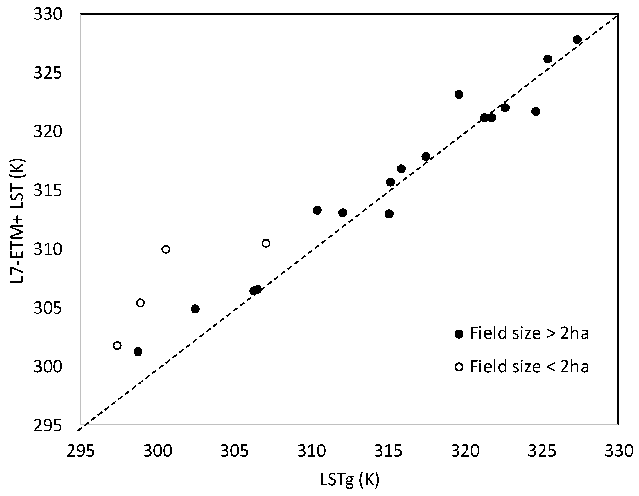
3.1. Ground Validation

The field scale assessment was performed using the ground data as a reference. IRT radiometric temperatures were corrected from atmospheric and emissivity effects, and average values for each 10-min transect/field were calculated. A total of 51 LSTg data were available for this study (Table 1). Measured LSTg values were in the range 297–327 K. The lowest values were observed for fully vegetated crops (grass, potato, or maize), whereas the largest values corresponded to bare soil, soil dominated crops (vineyard and almond orchard) and senescence cereals. Standard deviation of LSTg data per crop field were <±1.5 K in 90% of the dataset, with a maximum value of ±1.9 K, showing the thermal homogeneity of the fields and the thermal stability during the 10-min interval.
The methodology described above was applied to the six pairs of MODIS-S2 images listed in Table 1. Mean values of 5 × 5 high-resolution pixel arrays, centered in the location of the ground transects, were calculated and plotted against LSTg (see Figure 5). Disaggregated LST values ranged from 302 to 322 K, pointing to a certain limitation of the disaggregation technique to reproduce extreme low and high temperatures. Values of the standard deviation for the 5 x 5 pixel averages were <± 2.0 K.
All parcels in this study were provided with sprinkler irrigation system, except the vineyard and almond orchard, where drip irrigation was supplied. Irrigation was scheduled and frequently applied during the study period. For a few hours after an irrigation event, a cooling effect occurs consequence of the wetted surface. This effect is stressed when sprinklers are used. This was the case of 20% of our dataset, with 12 ground transects collected just a few hours/minutes after irrigation events. These points are plotted with non-filled circles in Figure 5. Note the evident overestimation of the disaggregated LST compared to LSTg values, with differences >10 K in some cases. These results reinforce Bisquert et al. [26] findings pointing a shortcoming of the method over wet soil areas.
Certain limitations were also observed for the highest LST values. By stablishing a threshold of 325 K, only five data were excluded corresponding to fallow and tilled barley or poppy.
Focusing on LST data lower than 325 K, and excluding points corresponding to recently irrigated conditions, a good agreement (r2 = 0.90) is observed between disaggregated LST10m and LSTg values (Figure 5). Differences range between ±4.0 K, with a systematic deviation of 0.2 K and a RMSD value of ±2.2 K (see Table 2). The kurtosis values (~−1) indicate a behavior close to the normal distribution, while the negligible skewness observed indicates a LST-difference distribution closely centered at 0.
The plot in Figure 6 superposes results obtained running the Bisquert et al. [1] algorithm. Good agreement is also observed by this original formulation, although some scatter is added, with an increase in the RMSD value up to ±2.7 K in this case.
MODIS LST values are superposed to plot in Figure 6 too, showing a large scatter (RMSD=±8.0 K) and discrepancies >10 K. This deviation is stressed for low temperatures registered in small size vegetated parcels that are surrounded by bare soil or other croplands with higher LST. This effect was already observed by Bisquert et al. [26].

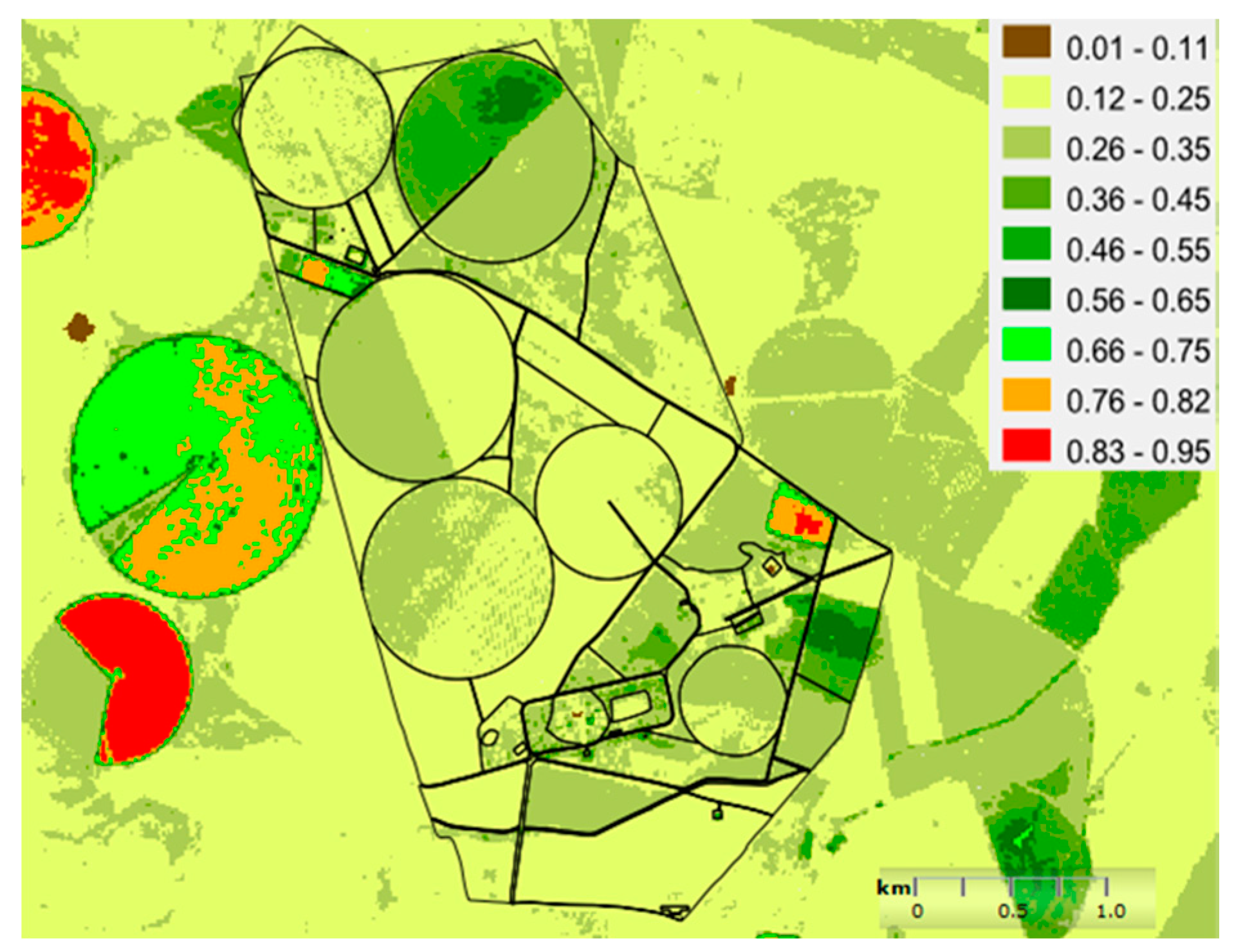
3.2. Distributed Assessment

Beyond the ground validation at a field scale, the model performance was assessed at a larger distributed scale by using the three concurrent Landsat-7/ETM+ images as a reference. The Single-Band Atmospheric Correction (SBAC) tool, recently introduced by Galve et al. [39], was used in this work for the correction of the TIR data.
Prior to the downscaling assessment, the feasibility of the Landsat-derived LST data needs to be tested. Ground data were also used to evaluate the Landsat-7/ETM+ LST estimates. The plot in Figure 7 shows the comparison between estimated and ground-measured LST values for a total of 21 data available for the three Landsat dates/images. Differences ranged within ± 3.5 K, except four cases corresponding to 1.1 and 1.2 sites. Note that these are small size parcels (<2 ha), for which the spatial resolution of Landsat 7/ETM+ is not fine enough, resulting in an overestimation of the LST values in these vegetated targets (potato and grass). Excluding these data from the analysis, a good matching with the 1:1 line was observed, with a coefficient of determination of r2 = 0.96. An average error of RMSD = ±1.8 K was obtained. These results are in agreement with those reported by Galve et al. [39], using data from 2015–2016 in this same agricultural area. A RMSD value of ±1.6 K was obtained by these authors using ground LST data measured in six of the crop fields within “Las Tiesas” experimental farm also used in the present work.
Note significant differences in terms of LST between MODIS and high-resolution sensors (Landsat or ASTER) up to 2–3 °C have been reported, induced by difference in the retrieval algorithm, atmospheric correction, sensor performance, acquisition time, view geometry, or spectral response function [10,42,43,44,45]. Weng et al. [44] pointed out that comparison of thermal data from different sensors requires some pre-processing procedure. In this work, the differences in the spectral characteristics and overpass time (20–30 min difference) between Landsat and MODIS were minimized by applying a normalization process to the Landsat bands [1]. The disaggregated LST10m were aggregated to the equivalent 30 m Landsat pixels (LST30m) by a 3 × 3 pixel averaging, based on the Stefan-Boltzmann law, following Gao et al. [20].
Figure 8 shows the comparison between the original 30-m LST derived from L7-ETM+, and LST disaggregation products at 10-m spatial resolution, for a subset of 10 × 10 km2 centered in the “Las Tiesas” experimental farm. Visual inspection points the significant improvement in the capacity to discriminate the different field borders. Although the real potential of the downscaling approach is revealed when focusing on parcels <5 ha, where 3 × 3 thermal pixels of L7-ETM+ can be hardly fit in, being these areas the main responsible of the scatter (r2 = 0.82) observed in the regression plot in Figure 9.
To quantify the performance of the downscaling approach at a full scene perspective, pixel-to-pixel differences were calculated at the 30 m spatial resolution for the selected subset of 10 × 10 km2 (Figure 9). Statistical metrics of the differences are listed in Table 3. Considering more than 270,000 pixel/data, an average RMSD of ±2.0 K was obtained, with a minor overestimation of 0.3 K.

4. Discussions

Agromomy management decisions based on TIR data need confidence in LST estimates. An absolute uncertainty <1.5 K is traditionally reported as a requirement [7,46]. The translation of this uncertainty to ET accuracy depends on the model but ranges between 10% and 20% [47,48]. Based on this threshold, the results obtained in this work (average RMSD = ±2.2 K) are encouraging. Additionally, the 10-m pixel size and the revisit frequency of the MODIS data, much better than the 3–5 days revisit frequency of S2A and S2B satellites, can fulfill the LST input requirements of the surface energy balance methods for a variety of hydrological, climatological or agricultural applications. At this point, no significant differences in the model performance were observed in connection with the collocation delay between the MODIS overpass and the Sentinel-2 image used, i.e., ±1-day mismatch seems not to have had an effect on the disaggregation.
With the new treatment of the residuals (RLST) introduced in this work, as part of the downscaling scheme, an improvement around 20% was obtained in the performance of the original formulation of the model [1] that simply included a Gaussian filter, as suggested by Anderson et al. [2].
Ground validation results are in agreement with those obtained by Bisquert et al. [26] using MODIS-Spot 5 pairs in this case. These authors reported a bias of 0.2 K and a RMSD of ±2.4 K based on the comparison between disaggregated 10-m LST and ground-measured LST values for 10 different dates and five different fields. Regarding the distributed assessment, our results are similar to the RMSD value of ±2.6 K reported by Bisquert et al. [26] at a scene scale. In a first work using MODIS-Landsat combination [1], these authors reported an average RMSD = ±2.0 K for disaggregated 60-m LST in this case.
In this context, Agam et al. [19] tested a sharpening model (TsHARP) over extensive corn/soybean fields in central Iowa, USA. RMSD values between ±0.7 and ±1.4 °C were obtained by sharpening down simulated MODIS thermal maps at 1000 m to 250 m and between ±1.8 and ±2.4 °C by sharpening simulated thermal Landsat maps from 60 and 120 m to a VNIR 30 m resolution. Also using TsHARP, Duan and Li [49] disaggregated MODIS LST from 1000 m to 90 m, with an uncertainty of ±2.7 °C. Jeganathan et al. [14] tested TsHARP from MODIS over a heterogeneous agricultural landscape in India, and found uncertainties ranging ±2–3 K, using ASTER thermal data as a reference. Eswar et al. [23] used a thermal sharpening technique with five different indices to downscale MODIS LST from 960 m to 120 m, and compared this with the Landsat 7 LST data at different sites in India. These authors found that NDVI/FVC showed better result for wet areas, whereas the Normalized Difference Water Index (NDWI) was found better for dry areas. Yang et al. [17] used the multiple linear regression models to downscale the aggregated Landsat TIRS (360 m) image to 90 m, using a relation of LST with multiple scale factors in an area of mixed land covers (water, vegetation, bare soil, impervious surface), and then compared with the pure Landsat LST. The result found was satisfactory with coefficient of determination of 0.87 and RMSD of ±1.13 K. Merlin et al. [10] used a time series of higher resolution Formosat-2 images to test a new disaggregation procedure of kilometric thermal data over an irrigated cropping area in northwestern Mexico during an agricultural season. RMSD values about ±3 °C were obtained by these authors.
Many of these previous studies already pointed larger uncertainties in disaggregated LST over irrigated lands [1,10,26]. This is a weekness that remains in the present work since, although affected, VNIR reflectivity data does not fully capture the cooling effect produced in a wetted surface. Therefore, the downscaling technique still fails at reproducing LST values for spots with an undergoing irrigation or recently irrigated targets. In an attempt to face these limitations, some works incorporate additional reflectance information in the regression algorithms. Gosh and Joshi [22] tested several regression algorithms using EO1-Hyperion hyperspectral data over different land use land cover scenes. These authors used three pairs of coincident Hyperion and Landsat 7-ETM+ images as a reference for the assessment. Liu et al. [24] compared the performances of a thermal disaggregation technique, based on three different indices: temperature vegetation dryness index (TVDI), NDVI and fractional vegetation cover (FVC), over a humid agriculture region. These authors found the smallest RMSD using TVDI, with an improvement of 0.2 K in comparison to the results obtained using NDVI or FVC. A similar reduction of the uncertainty in 0.2 K was obtained by Amazirh et al. [25], thanks to the inclusion of Sentinel-1 radar data, linked to surface soil moisture, in a new formulation to improve the LST disaggregation methodology. These authors used Sentinel-1 imagery to derive 100-m resolution LST, and the results were compared with Landsat LST, used as a reference over two heterogeneous sites (irrigated and rainfed). However, average RMSD values for the six dates of study resulted over ±3.0 K, with even worse accuracy during summer. So, further efforts are still required to improve this soil moisture integration. Further works should also explore the inclusion of additional Sentinel-2 bands in the shortwave infrared (SWIR) in the sharpening scheme, since they might account for vegetation and soil water content [50].
Another finding is this work is the difficulty of the downscaling approaches to reproduce excepcionally high LST when these conditions are constrained to small parcels in the image, and there is a lack of coarse original MODIS pixels showing this homogeneous thermal conditions. The modeled relationship LST-VNIR reflectivities may not fully cover these conditions, leading to an underestimation of LST.
Focusing on the combination of S3-S2 images, very few quantitative studies have been conducted. In a first attempt, Huryna et al. [28] applied TsHARP sharpening. These authors reported LST differences of ±1.3–1.5 K, when compared with sharpened to 60-m S3 temperature with reference Landsat 8 temperature at 60 m, with a positive bias of 0.3–0.6 K, depending on the study site. However, the lack of local measurements prevented these authors from conducting a ground assessment. Further research should merge Sentinel-2 and Sentinel-3 imagery and conduct robust assessment of the downscaling results. Collections of ground LST measurements under a variety of surface and environmental conditions are then required, and the dataset gathered in the framework of this work is potentially attractive for this aim.

5. Conclusions

This work adds to the previous literature dealing with thermal infrared downscaling. The 10-m LST maps generated from the combination MODIS-S2 can contribute to fill the gap until high spatial-temporal resolution TIR images are available. The linear relation NDVI-LST was adopted as a basis for the downscaling approach. Results obtained encourage the parametrization of the residual as a function of the NDVI as a key step in the algorithm (an improvement of 0.5 K was achieved). The variety of surface conditions and the wide range of NDVI and LST values in the semi-arid area of Barrax allowed a robust assessment of the downscaling approach. An average estimation error of ±2.2 K in LST10m resulted from the ground validation. This evaluation was reinforced by the pixel-to-pixel comparison of rescaled LST30m with Landsat-7/ETM+ LST estimates, showing a similar RMSD of ±2.0 K for the distributed assessment.
Findings in this study highlight the limitations of the methodology to capture the variability of extreme LST, and the problems in recently sprinkler irrigated fields. Results indicate the need for caution, since disaggregated LST under these conditions may result artificially higher than expected.
Despite the weaknesses, this work gives promising insights for the adaptation of this methodology to the tandem S3-S2 in coming works. Further research could also benefit from the ground LST dataset introduced in this paper for a comprehensive performance assessment.
Finally, note that the benefits of this research may extend to other applications, such as monitoring volcanic activity and wildfire, estimating evapotranspiration or assessing drought severity.

Author Contributions

Conceptualization, J.M.S.; Methodology, J.M.S. and J.M.G.; Resources, J.G.-P., R.L.-U. and A.C.; Software, J.M.G.; Validation, J.M.S., J.M.G. and R.N.; Writing—original draft, J.M.S.; Writing—review & editing, J.G.-P., R.L.-U., R.N. and A.C. All authors have read and agreed to the published version of the manuscript.

Funding

This research was funded by the Spanish Economy and Competitiveness Ministry, together with FEDER funds (project CGL2016-80609-R), the Education and Science Council (JCCM, Spain) (project SBPLY/17/180501/000357), the European Commission (SUPROMED project, N° 1813), and Juan de la Cierva Research Grant of Galve (FJCI-2015-24876).

Acknowledgments

We thank the ITAP-FUNDESCAM and the Thermal Remote Sensing Group of University of Valencia for the logistic support in the experimental campaigns (MINECO-FEDER, EU projects AGL2017-83738-C3-3-R and CGL2015-64268-R).

Conflicts of Interest

The authors declare no conflict of interest.

References

  1. Bisquert, M.; Sánchez, J.M.; Caselles, V. Evaluation of Disaggregation Methods for Downscaling Modis Land Surface Temperature to Landsat Spatial Resolution in Barrax Test Site. IEEE J. Sel. Top. Appl. Earth Obs. Remote Sens. 2016, 9, 1430–1438. [Google Scholar] [CrossRef]
  2. Anderson, M.C.; Kustas, W.P.; Alfieri, J.G.; Gao, F.; Hain, C.; Prueger, J.H.; Evett, S.; Colaizzi, P.; Howell, T.; Chávez, J.L. Mapping Daily Evapotranspiration at Landsat Spatial Scales During the BEAREX’08 Field Campaign. Adv. Water Resour. 2012, 50, 162–177. [Google Scholar] [CrossRef] [Green Version]
  3. Ha, W.; Gowda, P.; Howell, T. A Review of Downscaling Methods for Remote Sensing-Based Irrigation Management: Part I. Irrig. Sci. 2013, 31, 831–850. [Google Scholar] [CrossRef]
  4. Guzinski, R.; Anderson, M.C.; Kustas, W.P.; Nieto, H.; Sandholt, I. Using a Thermal Based Two Source Energy Balance Model with Time-Differencing to Estimate Surface Energy Fluxes with Day-Night MODIS Observations. Hydrol. Earth Syst. Sci. 2013, 17, 2809–2825. [Google Scholar] [CrossRef] [Green Version]
  5. Fisher, J.B. The future of evapotranspiration: Global Requirements for Ecosystem Functioning, Carbon and Climate Feedbacks, Agricultural Management, and Water Resources. Water Resour. Res. 2017, 53, 2618–2626. [Google Scholar] [CrossRef]
  6. Hulley, G.; Hook, S.; Fisher, J.; Lee, C. Ecostress, A NASA Earth-Ventures Instrument for Studying Links Between the Water Cycle and Plant Health over the Diurnal Cycle. In Proceedings of the 2017 IEEE International Geoscience and Remote Sensing Symposium (IGARSS), Fort Worth, TX, USA, 23–28 July 2017; pp. 5494–5496. [Google Scholar] [CrossRef]
  7. Sobrino, J.A.; Jiménez-Muñoz, J.C.; Soria, G.; Ruescas, A.B.; Danne, O.; Brockmann, C.; Ghent, D.; Remedios, J.; North, P.; Merchant, C.; et al. Synergistic Use of MERIS and AATSR as a Proxyfor Estimating Land Surface Temperature from Sentinel-3 Data. Remote Sens. Environ. 2016, 179, 149–161. [Google Scholar] [CrossRef]
  8. Guzinski, R.; Nieto, H. Evaluating the Feasibility of Using Sentinel-2 and Sentinel-3 Satellites for High-Resolution Evapotranspiration Estimations. Remote Sens. Environ. 2019, 221, 157–172. [Google Scholar] [CrossRef]
  9. He, B.-J.; Zhao, Z.-Q.; Shen, L.-D.; Wang, H.-B.; Li, L.-G. An Approach to Examining Performances of Cool/Hot Sources in Mitigating/Enhancing Land Surface Temperature under Different Temperature Backgrounds Based on Landsat 8 Image. Sustain. Cities Soc. 2019, 44, 416–427. [Google Scholar] [CrossRef]
  10. Merlin, O.; Duchemin, B.; Hagolle, O.; Jacob, F.; Coudert, B.; Chehbouni, G.; Dedieu, G.; Garatuza, J.; Kerr, Y. Disaggregation of MODIS Surface Temperature over an Agricultural Area Using a Time Series of Formosat-2 Images. Remote Sens. Environ. 2010, 114, 2500–2512. [Google Scholar] [CrossRef] [Green Version]
  11. Lagouarde, J.-P. The MISTIGRI Thermal Infrared Project: Scientific Objectives and Mission Specifications. Int. J. Remote Sens. 2013, 34, 3437–3466. [Google Scholar] [CrossRef]
  12. Koetz, B.; Berger, M.; Blommaert, J.; Del Bello, U.; Drusch, M.; Duca, R.; Gascon, F.; Ghent, D.; Hoogeveen, J.; Hook, S.; et al. Copernicus High Spatio-Temporal Resolution Land Surface Temperature Mission: Mission Requirements Document; ESA: Noordwijk, The Netherlands, 2019. [Google Scholar]
  13. Lagouarde, J.-P. The Indian-French Trishna Mission: Earth Observation in the Thermal Infrared with High Spatio-Temporal Resolution. In Proceedings of the IGARSS 2018—2018 IEEE International Geoscience and Remote Sensing Symposium, Valencia, Spain, 22–27 July 2018; pp. 4078–4081. [Google Scholar] [CrossRef]
  14. Jeganathan, C.; Hamm, N.A.S.; Mukherjee, S.; Atkinson, P.M.; Raju, P.L.N.; Dadhwal, V.K. Evaluating a Thermal Image Sharpening Model over a Mixed Agricultural Landscape in India. Int. J. Appl. Earth Obs. Geoinform. 2011, 13, 178–191. [Google Scholar] [CrossRef]
  15. Zhan, W.; Chen, Y.; Zhou, J.; Wang, J.; Liu, W.; Voogt, J.; Zhu, Z.; Quan, J.; Li, J. Disaggregation of Remotely Sensed Land Surface Temperature: Literature Survey, Taxonomy, Issues, and Caveats. Remote Sens. Environ. 2013, 131, 119–139. [Google Scholar] [CrossRef]
  16. Cammalleri, C.; Anderson, M.C.; Gao, F.; Hain, C.R.; Kustas, W.P. A Data Fusion Approach for Mapping Daily Evapotranspiration at Field Scale. Water Resour. Res. 2013, 49, 4672–4686. [Google Scholar] [CrossRef]
  17. Yang, Y.; Li, X.; Pan, X.; Zhang, Y.; Cao, C. Downscaling Land Surface Temperature in Complex Regions by Using Multiple Scale Factors with Adaptive Thresholds. Sensors 2017, 17, 744. [Google Scholar] [CrossRef] [Green Version]
  18. Kustas, W.P.; Norman, J.M.; Anderson, M.C.; French, A.N. Estimating Subpixel Surface Temperatures and Energy Fluxes from the Vegetation Index–Radiometric Temperature Relationship. Remote Sens. Environ. 2003, 85, 429–440. [Google Scholar] [CrossRef]
  19. Agam, N.; Kustas, W.P.; Anderson, M.C.; Li, F.; Neale, C.M.U. A Vegetation Index Based Technique for Spatial Sharpening of Thermal Imagery. Remote Sens. Environ. 2007, 107, 545–558. [Google Scholar] [CrossRef]
  20. Gao, F.; Kustas, W.; Anderson, M. A Data Mining Approach for Sharpening Thermal Satellite Imagery over Land. Remote Sens. 2012, 4, 3287–3319. [Google Scholar] [CrossRef] [Green Version]
  21. Bindhu, V.M.; Narasimhan, B.; Sudheer, K.P. Development and Verification of a Non-Linear Disaggregation Method (NL-Distrad) to Downscale MODIS Land Surface Temperature to the Spatial Scale of Landsat Thermal Data to Estimate Evapotranspiration. Remote Sens. Environ. 2013, 135, 118–129. [Google Scholar] [CrossRef]
  22. Ghosh, A.; Joshi, P.K. Hyperspectral Imagery for Disaggregation of Land Surface Temperature with Selected Regression Algorithms over Different Land Use Land Cover Scenes. ISPRS J. Photogramm. Remote Sens. 2014, 96, 76–93. [Google Scholar] [CrossRef]
  23. Eswar, R.; Sekhar, M.; Bhattacharya, B.K. Disaggregation of LST over India: Comparative Analysis of Different Vegetation Indices. Int. J. Remote Sens. 2016, 37, 1035–1054. [Google Scholar] [CrossRef]
  24. Liu, K.; Wand, S.; Li, X.; Li, Y.; Zhang, B.; Zhai, R. The Assessment of Different Vegetation Indices for Spatial Disaggregating of Thermal Imagery over the Humid Agricultural Region. Int. J. Remote Sens. 2019, 41, 1907–1926. [Google Scholar] [CrossRef]
  25. Amazirh, A.; Merlin, O.; Er-Raki, S. Including Sentinel-1 Radar Data to Improve the Disaggregation of MODIS Land Surface Temperature Data. ISPRS J. Photogramm. Remote Sens. 2019, 150, 11–26. [Google Scholar] [CrossRef]
  26. Bisquert, M.; Sánchez, J.M.; López-Urrea, R.; Caselles, V. Estimating High Resolution Evapotranspiration from Disaggregated Thermal Images. Remote Sens. Environ. 2016, 187, 423–433. [Google Scholar] [CrossRef]
  27. Sobrino, J.; Jiménez-Muñoz, J.; Brockmann, C.; Ruescas, A.; Danne, O.; North, P.; Heckel, A.; Davies, W.; Berger, M.; Merchant, C.; et al. Land Surface Temperature Retrieval from Sentinel 2 and 3 Missions. In Proceedings of the Sentinel-3 OLCI/SLSTR and MERIS/(A)ATSR Workshop, Frascati, Italy, 15–19 October 2012; Ouwehand, L., Ed.; ESA Communications: Oakville, ON, Canada, 2013. ISBN 9789290922759 (SP-711). [Google Scholar]
  28. Huryna, H.; Cohen, Y.; Karnieli, A.; Panov, N.; Kustas, W.P.; Agam, N. Evaluation of Tsharp Utility for Thermal Sharpening of Sentinel-3 Satellite Images Using Sentinel-2 Visual Imagery. Remote Sens. 2019, 11, 2304. [Google Scholar] [CrossRef] [Green Version]
  29. Moreno, J.F. “The SPECTRA Barrax campaign (SPARC): Overview and First Results from CHRIS Data”. In Proceedings of the Second CHRIS/Proba Workshop, ESA SP-578, Frascati, Italy, 28–30 April 2004. [Google Scholar]
  30. Sobrino, J.A. Thermal Remote Sensing in the Framework of the SEN2FLEX Project: Field Measurements, Airborne Data and Applications. Int. J. Remote Sens. 2008, 29, 4961–4991. [Google Scholar] [CrossRef]
  31. Latorre, C. Seasonal Monitoring of FAPAR Over the Barrax Cropland Site in Spain, In Support of the Validation of PROBA-V Products at 333 m. In Proceedings of the Recent Advances in Quantitative Remote Sensing, Torrent, Spain, 22–26 September 2014; pp. 431–435. [Google Scholar]
  32. Niclòs, R.; Pérez-Planells, L.l.; Coll, C.; Valiente, J.A.; Valor, E. Evaluation of the S-NPP VIIRS Land Surface Temperature Product Using Ground Data Acquired by an Autonomous System at a Rice Paddy. ISPRS J. Photogramm. Remote Sens. 2018, 135, 1–12. [Google Scholar] [CrossRef]
  33. Sánchez, J.M.; López-Urrea, R.; Rubio, E.; González-Piqueras, J.; Caselles, V. Assessing Crop Coefficients of Sunflower and Canola Using Two-Source Energy Balance and Thermal Radiometry. Agric. Water Manag. 2014, 137, 23–29. [Google Scholar] [CrossRef]
  34. Gillespie, A.; Rokugawa, S.; Matsunaga, T.; Cothern, J.S.; Hook, S.; Kahle, A.B. A Temperature and Emissivity Separation from Advanced Spaceborne Thermal Emission and Reflection Radiometer (ASTER) Images. IEEE Trans. Geosci. Remote Sens. 1998, 36, 1113–1126. [Google Scholar] [CrossRef]
  35. Sánchez, J.M.; French, A.N.; Mira, M.; Hunsaker, D.J.; Thorp, K.R.; Valor, E.; Caselles, V. Thermal Infrared Emissivity Dependence on Soil Moisture in Field Conditions. IEEE Trans. Geosci. Remote Sens. 2011, 49, 4652–4659. [Google Scholar] [CrossRef]
  36. Legrand, M.; Pietras, C.; Brogniez, G.; Haeffelin, M.; Abuhassan, N.K.; Sicard, M.A. high-Accuracy Multiwavelength Radiometer for in Situ Measurements in the Thermal Infrared. Part I: Characterization of the Instrument. J. Atmos. Ocean Technol. 2000, 17, 1203–1214. [Google Scholar] [CrossRef]
  37. Wolfe, R.E.; Nishihama, M.; Fleig, A.J.; Kuyper, J.A.; Roy, D.P.; Storey, J.C.; Patt, F.S. Achieving Sub-Pixel Geolocation Accuracy in Support of MODIS Land Science. Remote Sens. Environ. 2002, 83, 31–49. [Google Scholar] [CrossRef]
  38. Wan, Z. New Refinements and Validation of the MODIS Land Surface Temperature/Emissivity Products. Remote Sens. Environ. 2008, 112, 59–74. [Google Scholar] [CrossRef]
  39. Galve, J.M.; Sánchez, J.M.; Coll, C.; Villodre, J. A New Single-Band Pixel-By-Pixel Atmospheric Correction Method to Improve the Accuracy in Remote Sensing Estimates of LST. Application to Landsat 7-ETM+. Remote Sens. 2018, 10, 826. [Google Scholar] [CrossRef] [Green Version]
  40. Willmott, C.J. Some Comments on the Evaluation of Model Performance. Bull. Am. Meteorol. Soc. 1982, 63, 1309–1313. [Google Scholar] [CrossRef] [Green Version]
  41. Schneider, P.; Ghent, D.; Corlett, G.; Prata, F.; Remedios, J. Land Surface Temperature Validation Protocol; ESA: Noordwijk, The Netherlands, 2012. [Google Scholar]
  42. Essa, W.; Verbeiren, B.; van der Kwast, J.; Batelaan, O. Improved DisTrad for Downscaling Thermal MODIS Imagery over Urban Areas. Remote Sens. 2017, 9, 1243. [Google Scholar] [CrossRef] [Green Version]
  43. Liu, Y.; Hiyama, T.; Yamaguchi, Y. Scaling of Land Surface Temperature Using Satellite Data: A Case Examination on ASTER and MODIS Products over a Heterogeneous Terrain Area. Remote Sens. Environ. 2006, 105, 115–128. [Google Scholar] [CrossRef]
  44. Weng, Q.; Fu, P.; Gao, F. Generating Daily Land Surface Temperature at Landsat Resolution by Fusing Landsat and MODIS Data. Remote Sens. Environ. 2014, 145, 55–67. [Google Scholar] [CrossRef]
  45. Brown, M.E.; Pinzon, J.E.; Didan, K.; Morisette, J.T.; Tucker, C.J. Evaluation of the Consistency of Long-Term NDVI Time Series Derived from AVHRR, SPOT-Vegetation, Seawifs, MODIS, and Landsat ETM+ Sensors. IEEE Trans. Geosci. Remote Sens. 2006, 44, 1787–1793. [Google Scholar] [CrossRef]
  46. Ghent, D.J.; Corlett, G.K.; Göttsche, F.M.; Remedios, J.J. Global Land Surface Temperature from the Along Track Scanning Radiometers. J. Geophys. Res. Atmos. 2017, 122, 12167–12193. [Google Scholar] [CrossRef] [Green Version]
  47. Allen, R.; Tasumi, M.; Trezza, R. Satellite-Based Energy Balance for Mapping Evapotranspiration with Internalized Calibration (METRIC)\97 Model. J. Irrig. Drain. Eng. 2007, 133, 380–394. [Google Scholar] [CrossRef]
  48. Sánchez, J.M.; Kustas, W.P.; Caselles, V.; Anderson, M. Modelling Surface Energy Fluxes over Maize Using a Two-Source Patch Model and Radiometric Soil and Canopy Temperature Observations. Remote Sens. Environ. 2008, 112, 1130–1143. [Google Scholar] [CrossRef]
  49. Duan, S.-B.; Li, Z.L. Spatial Downscaling of MODIS Land Surface Temperatures Using Geographically Weighted Regression: Case Study in Northern China. IEEE Trans. Geosci. Remote Sens. 2016, 54, 6458–6469. [Google Scholar] [CrossRef]
  50. Sadeghi, M.; Babaeian, E.; Tuller, M.; Jones, S.B. The Optical Trapezoid Model: A Novel Approach to Remote Rensing of Soil Moisture Applied to Sentinel-2 and Landsat-8 Observations. Remote Sens. Environ. 2017, 198, 52–68. [Google Scholar] [CrossRef] [Green Version]
Figure 1. Overview of “Las Tiesas” experimental farm. Measurement sites are located over a S2 false color composition corresponding to date 25 July 2018. Labels for the different study fields are explained in the adjacent Table, together with indication of crop type and field size.
Remotesensing 12 01453 g001
Figure 2. Sentinel-2 Normalized Difference Vegetation Index (NDVI) image of “Las Tiesas” farm, corresponding to date 25 July 2018.
Remotesensing 12 01453 g002
Figure 3. Distribution of the Sentinel-2 NDVI values for the different sites labeled in Figure 1, and the images/dates listed in Table 1.
Remotesensing 12 01453 g003
Figure 4. Flowchart of the downscaling methodology, including the different processing steps, inputs and outputs. Variable descriptions are included in the text.
Remotesensing 12 01453 g004
Figure 5. Linear regression between disaggregated LST10m and ground-measured values (LSTg). Crop fields under recently irrigated conditions are labeled with a non-filled circle. Outlier high LST values are labeled with triangles. Dashed line represents the 1:1 agreement.
Remotesensing 12 01453 g005
Figure 6. Disaggregated LST10m (dots) and Moderate Resolution Imaging Spectroradiometer (MODIS) LST (crosses) versus ground LST measurements (LSTg). Non-filled dots represent results using the original Bisquert et al. [1] formulation of the downscaling approach. Error bars are not included in this figure for cleanliness. Dashed line represents the 1:1 agreement.
Remotesensing 12 01453 g006
Figure 7. Linear adjustment between L7-ETM+ estimates and ground-measured LST values. Data collected in Sites 1.1 and 1.2 (field extension <2 ha) are labeled with non-filled dots. Dashed line represents the 1:1 agreement.
Remotesensing 12 01453 g007
Figure 8. Disaggregated LST10m (left column), LST derived from original 30 m L7-ETM+ Thermal InfraRed (TIR) band (center), and MOD11A1_LST product (right column). Examples corresponding to dates 9 July 2018 (up), 16 July 2018 (middle), and 25 July 2018 (bottom).
Remotesensing 12 01453 g008
Figure 9. Disaggregated LST30m versus L7-ETM+ LST for the full dataset (left). Dashed line represents the 1:1 agreement. Histograms of pixel-to-pixel differences between disaggregated LST30m products and LST estimates from L7-ETM+ images for three concurrent MODIS and Landsat-7 overpasses (right).
Remotesensing 12 01453 g009
Table 1. List of satellite images used in this study, with indication of overpass time. Number of crop fields where LSTg data were measured per date is included (N). Meteorological conditions in the area at the overpass time are also listed: air temperature (Ta), relative humidity (Hr) and wind speed (u). All dates correspond to the year 2018.
Terra/MODIS Sentinel-2 Landsat-7/ETM+LSTg DataTaHru
DateTimeViewing Angle (°)(A/B)(Path/Row)-Time(N)(°C)(%)(ms−1)
22 June 11:1419A (22 June) no image928.233.12.4
5 July 11:1710B (5 July)no image923.937.13.9
9 July 11:020A (10 July)(199/33)-10:32730.133.01.5
16 July 11:0812B (15 July)(200/33)-10:38824.337.36.4
23 July 11:1424A (23 July)no image929.734.11.5
25 July 11:022B (25 July)(199/33)-10:32928.637.62.0
Table 2. Quantitative analysis of the differences between disaggregated LST or MODIS LST, and ground-measured LST data. The statistics include: mean bias (Bias); standard deviation (SD); mean absolute deviation (MAD); Mean Absolute Deviation in Percentage (MADP), obtained as the MAD divided by the mean observed value; root mean square difference (RMSD); coefficient of determination (r2); median bias (Me); robust standard deviation (RSD); robust RMSD (R−RMSD); skewness (S); and kurtosis (K).
N = 34Min (K)Max (K)Bias (K)SD (K)MAD (K)MADP (%)RMSD (K)r2Me (K)RSD (K)R-RMSD (K)SK
LST10m−3.63.90.22.21.90.62.20.900.22.82.8−0.04−1.2
LST10m (Bisquert et al. [1])−4.55.70.42.72.30.72.70.900.53.33.40.06−0.8
LST_MOD−4.220.54.46.85.41.78.00.101.27.77.81.10.3
Table 3. Quantitative analysis of the differences plotted in Figure 9. Statistical metrics as defined in Table 2.
NBias (K)SD (K)MAD (K)MADP (%)RMSD (K)r2Me (K)RSD (K)R-RMSD (K)
9 July678260.72.51.90.62.60.550.52.82.8
16 July116015−0.41.41.20.41.40.63−0.61.71.8
25 July908040.91.81.50.52.00.750.82.22.3
Average2746430.31.91.40.52.00.820.0102.12.1

