Small-Object Detection in Remote Sensing Images with End-to-End Edge-Enhanced GAN and Object Detector Network


Abstract
1. Introduction
1.1. Problem Description and Motivation
1.2. Contributions of Our Method
2. Related Works
2.1. Image Super-Resolution
2.2. Object Detection
2.3. Super-Resolution Along with Object Detection
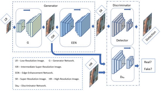
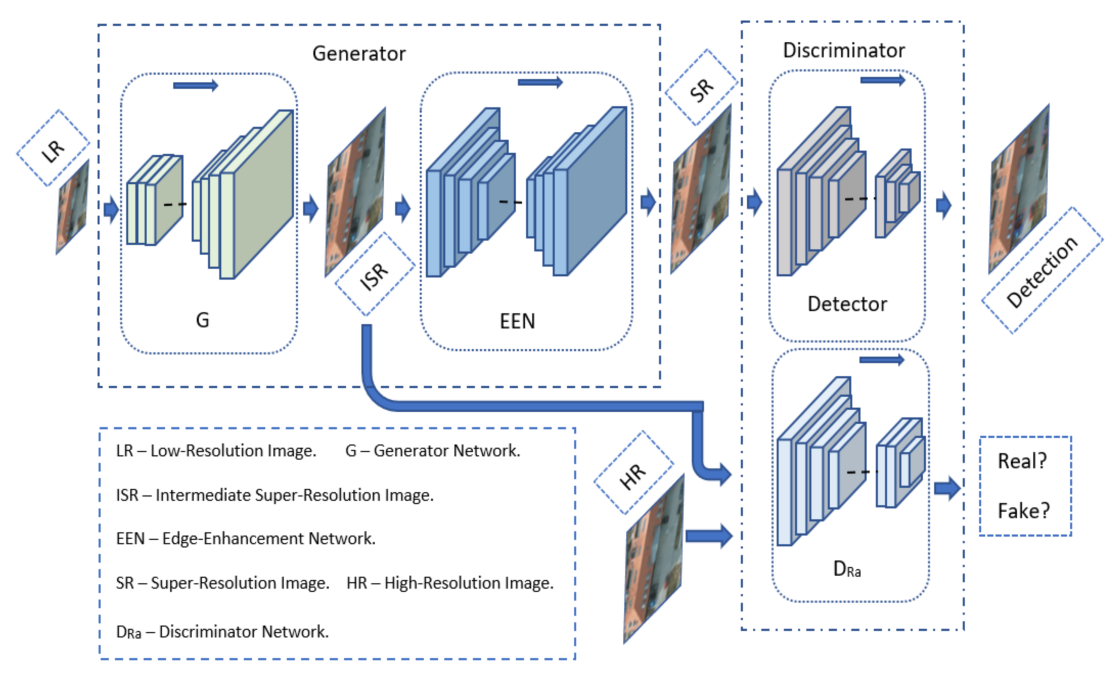
3. Method
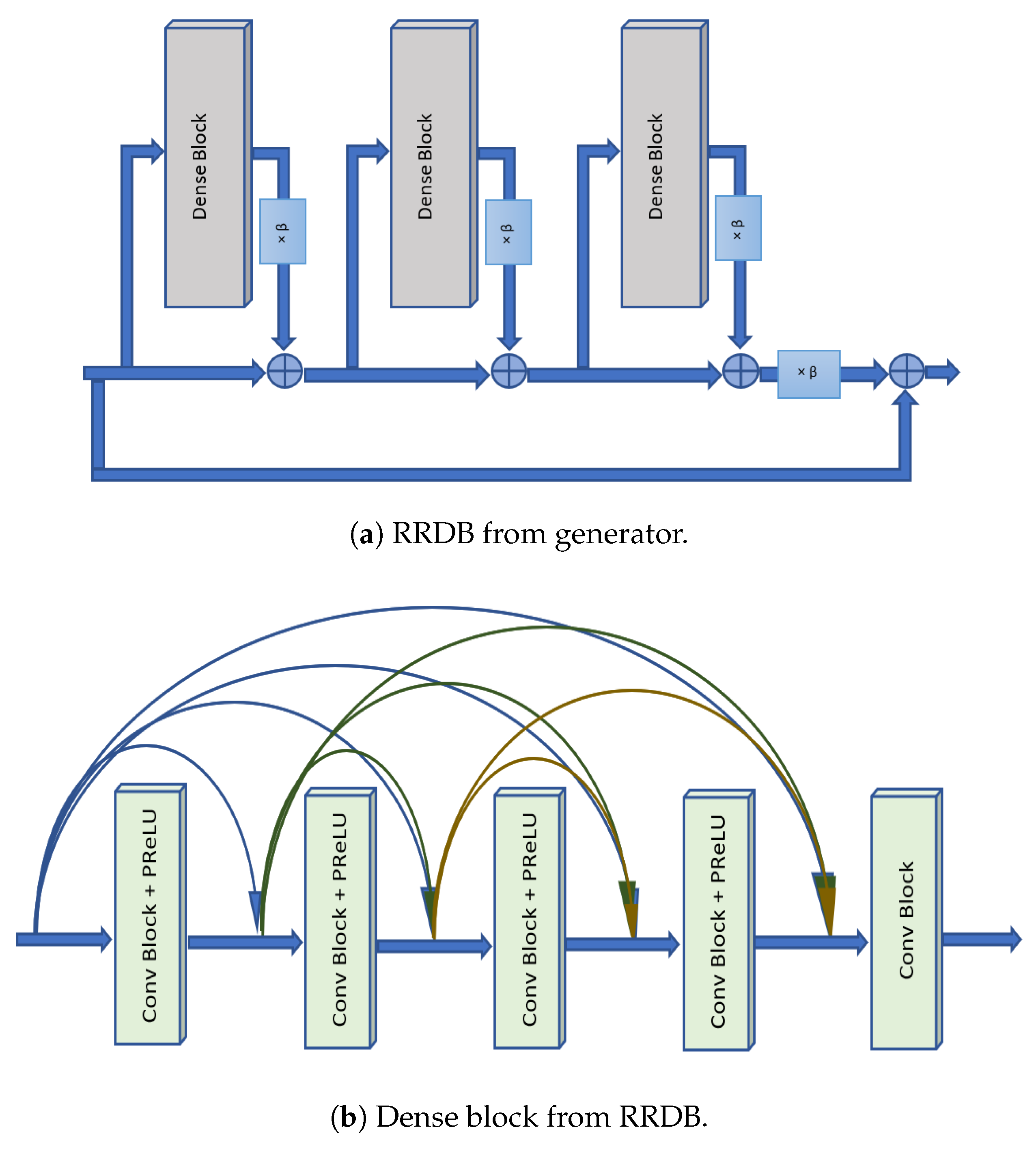
3.1. Generator
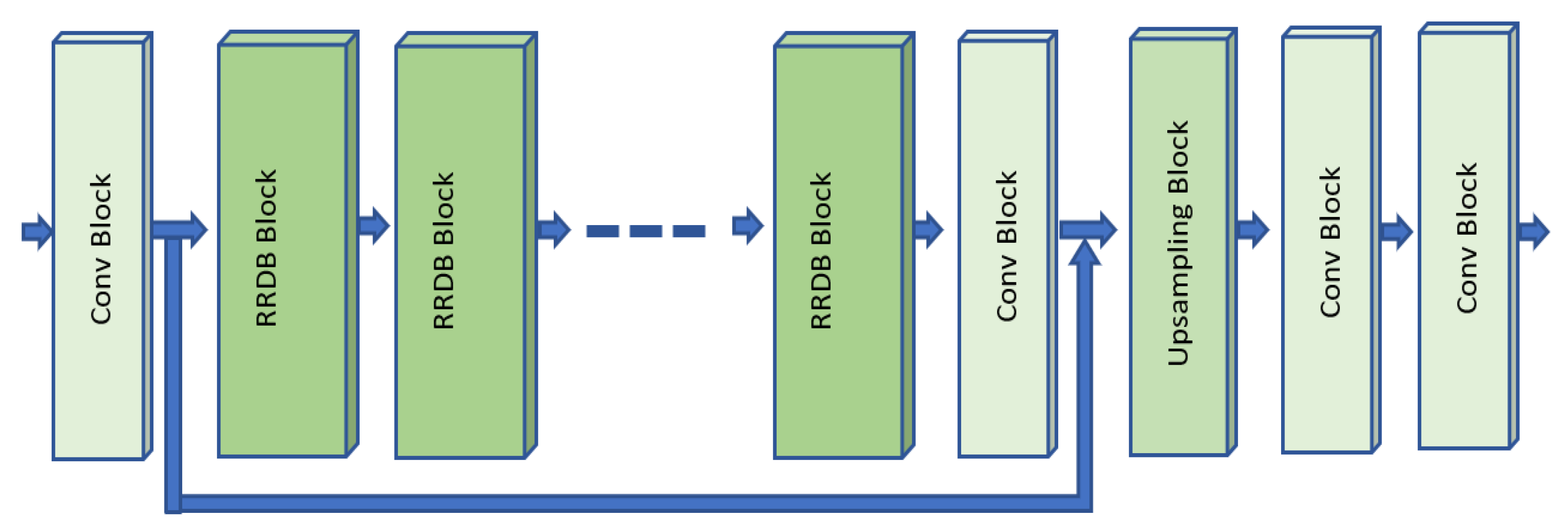
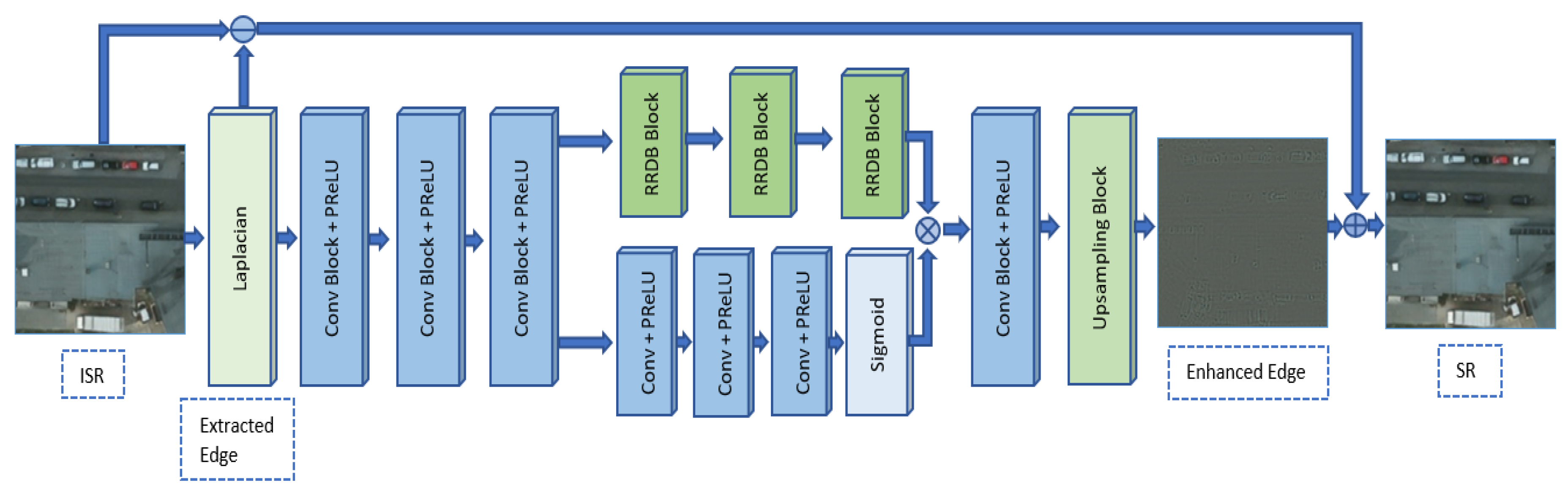
3.1.1. Generator Network G
3.1.2. Edge-Enhancement Network EEN
3.2. Discriminator
3.2.1. Faster R-CNN
3.2.2. SSD
3.2.3. Loss of the Discriminator
3.3. Training
3.3.1. Separate Training
3.3.2. End-to-End Training
4. Experiments
4.1. Datasets
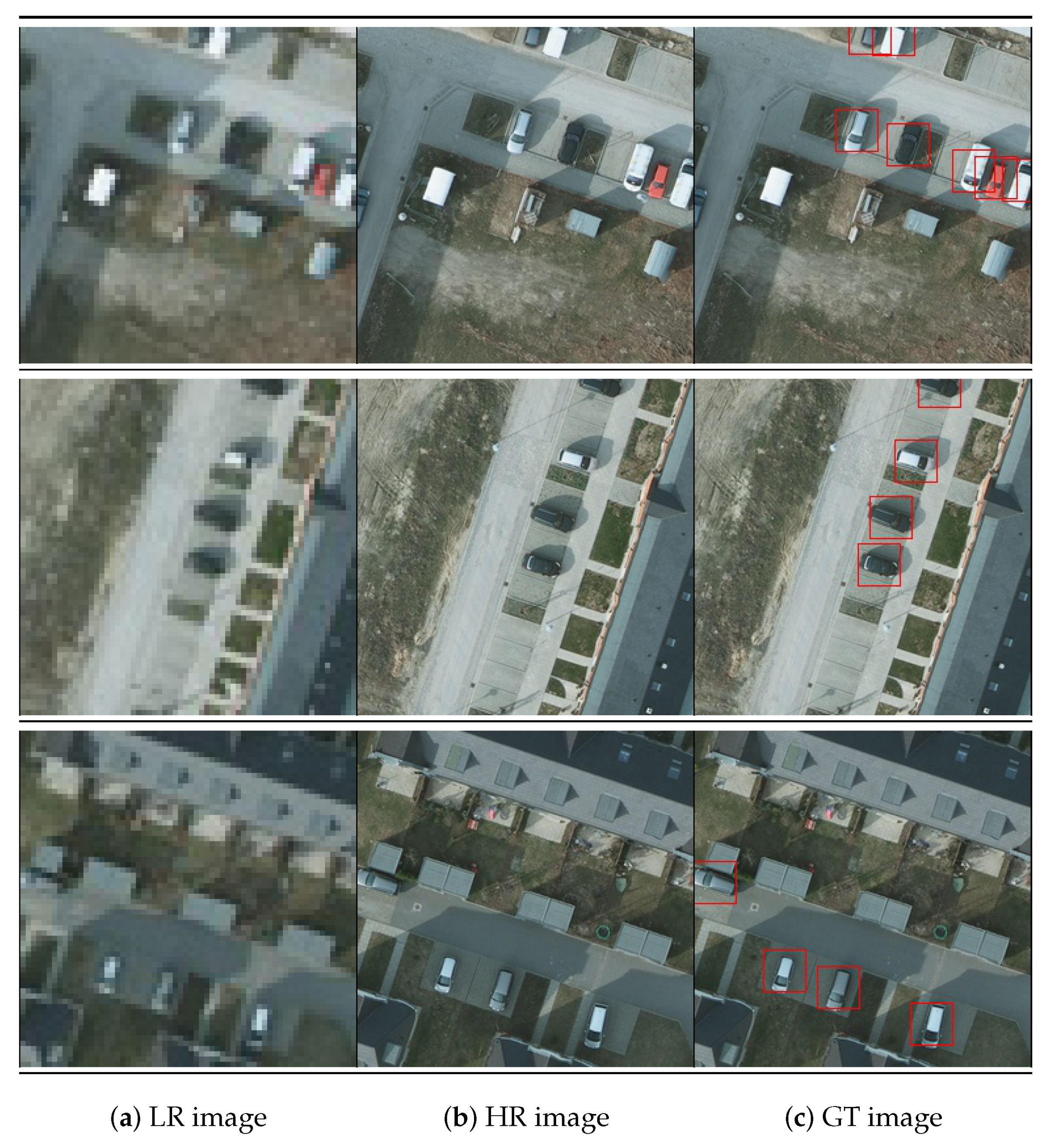
4.1.1. Cars Overhead with Context Dataset
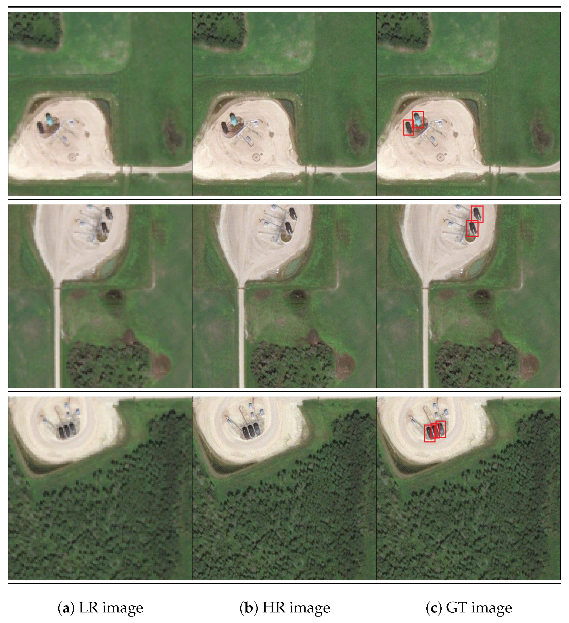
4.1.2. Oil and Gas Storage Tank Dataset
4.2. Evaluation Metrics for Detection
4.3. Results
4.3.1. Detection without Super-Resolution
4.3.2. Separate Training with Super-Resolution
4.3.3. End-to-End Training with Super-Resolution
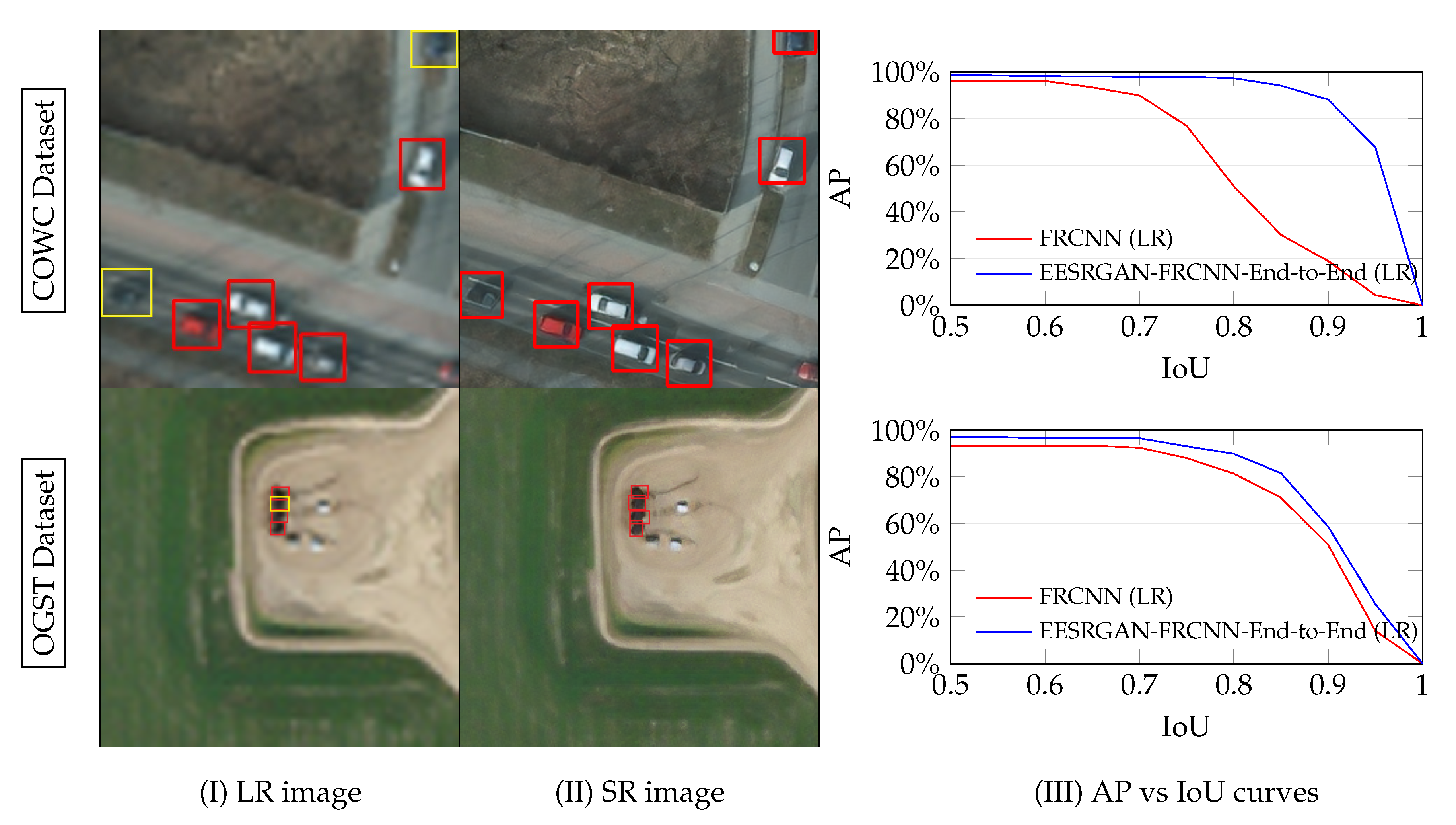
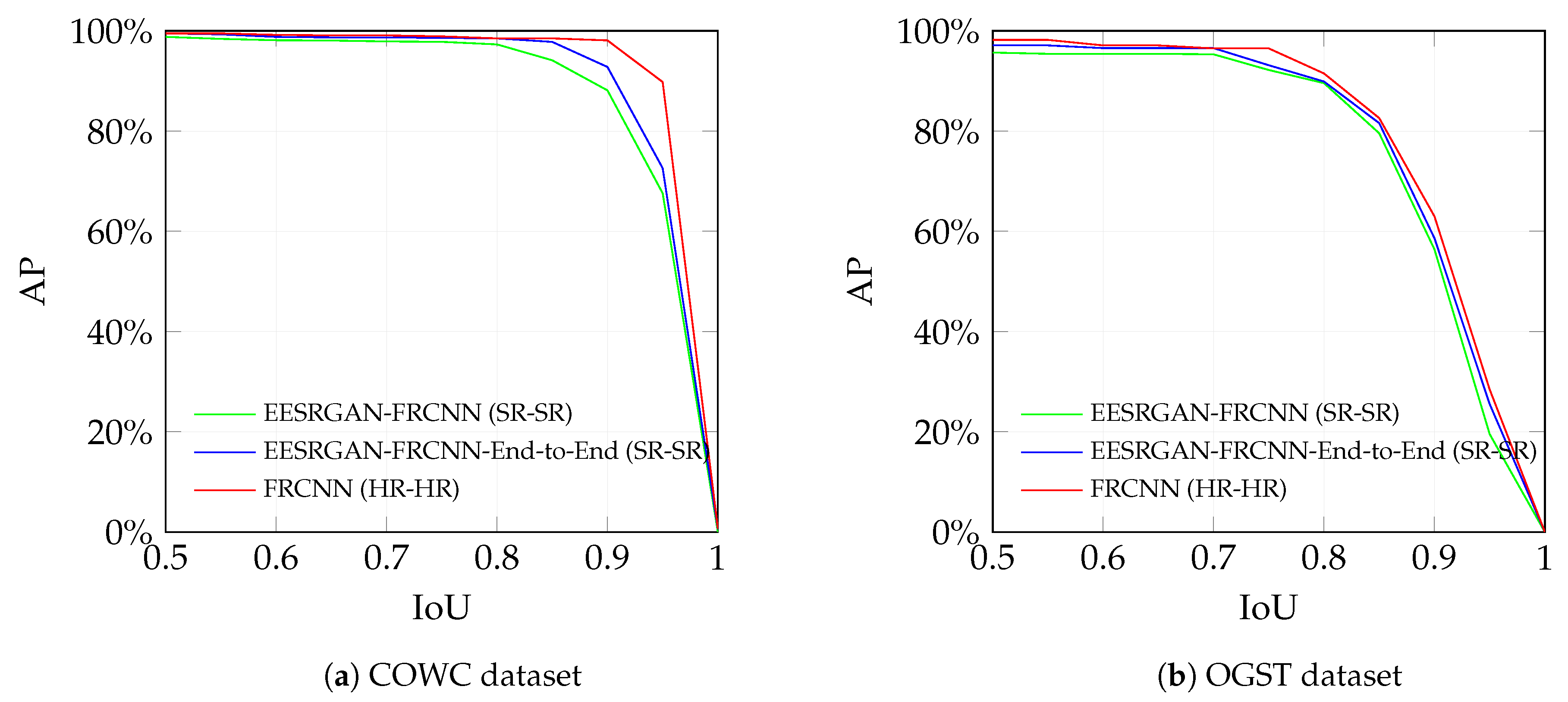
4.3.4. AP Versus IoU Curve
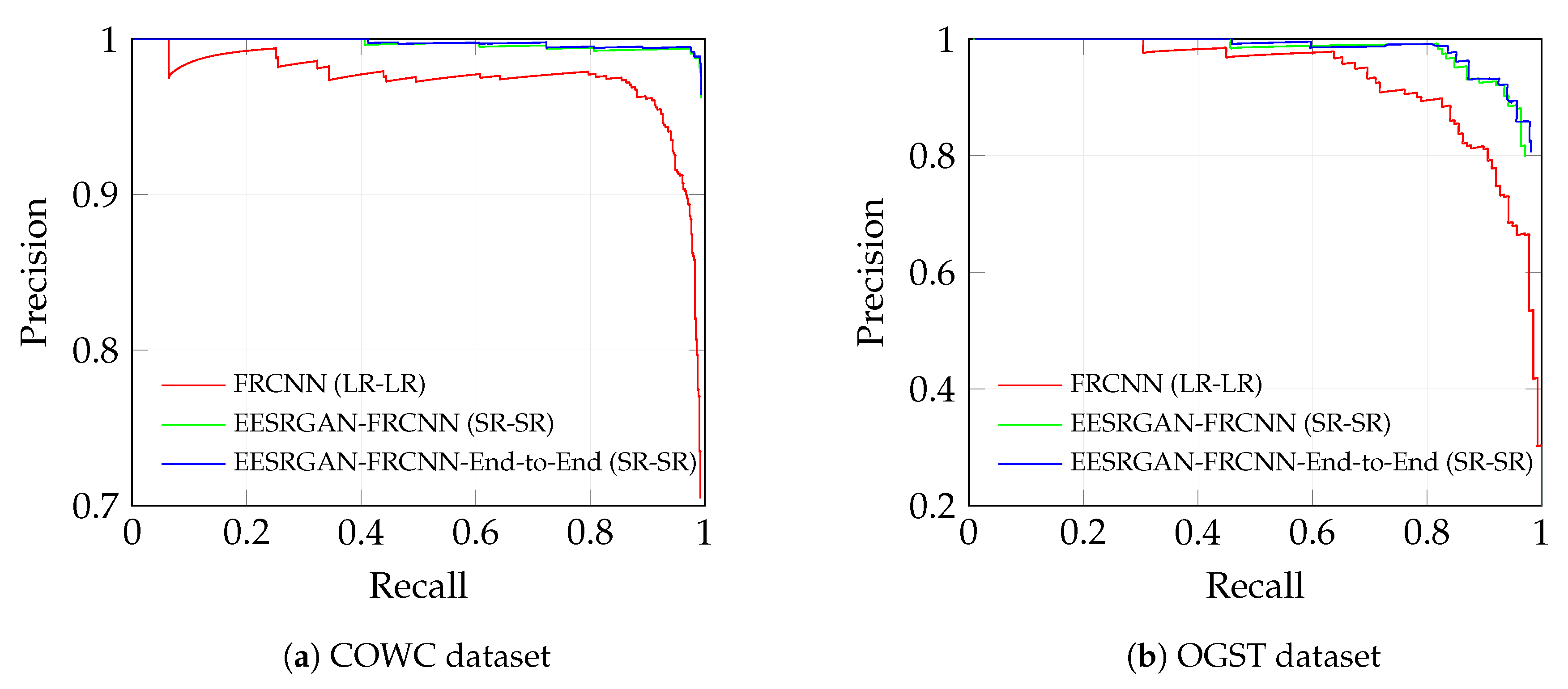
4.3.5. Precision Versus Recall
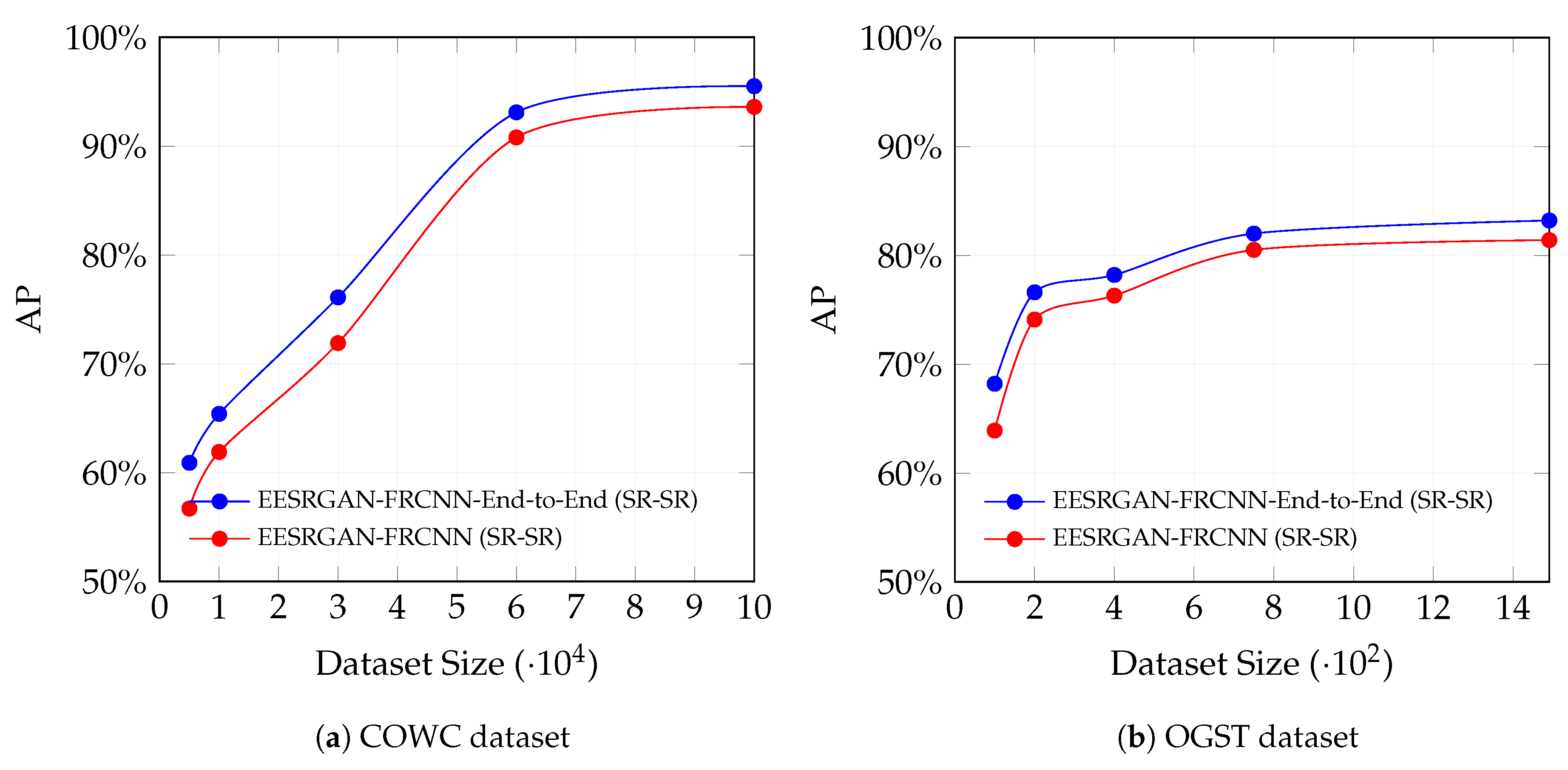
4.3.6. Effects of Dataset Size
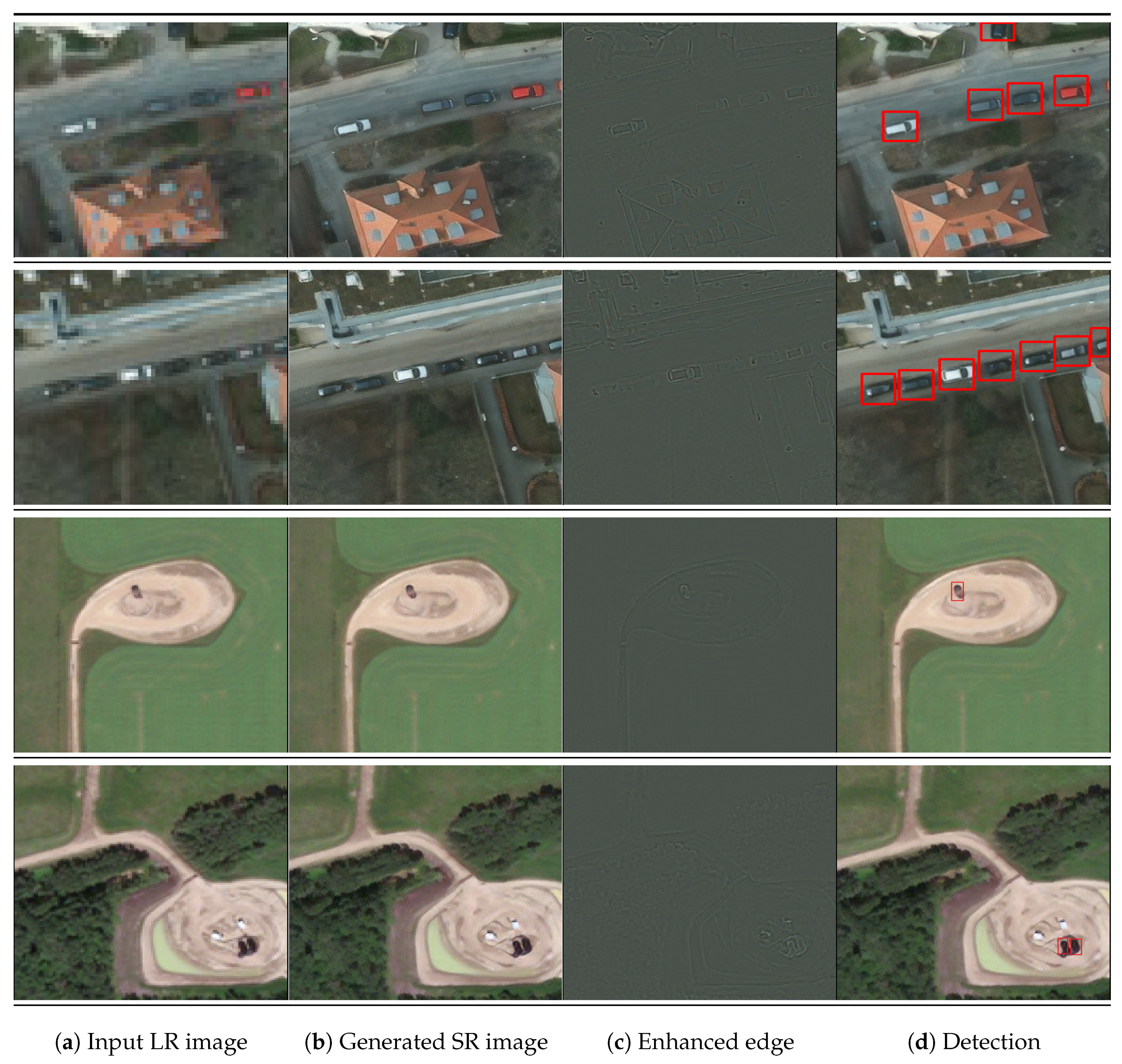
4.3.7. Enhancement and Detection
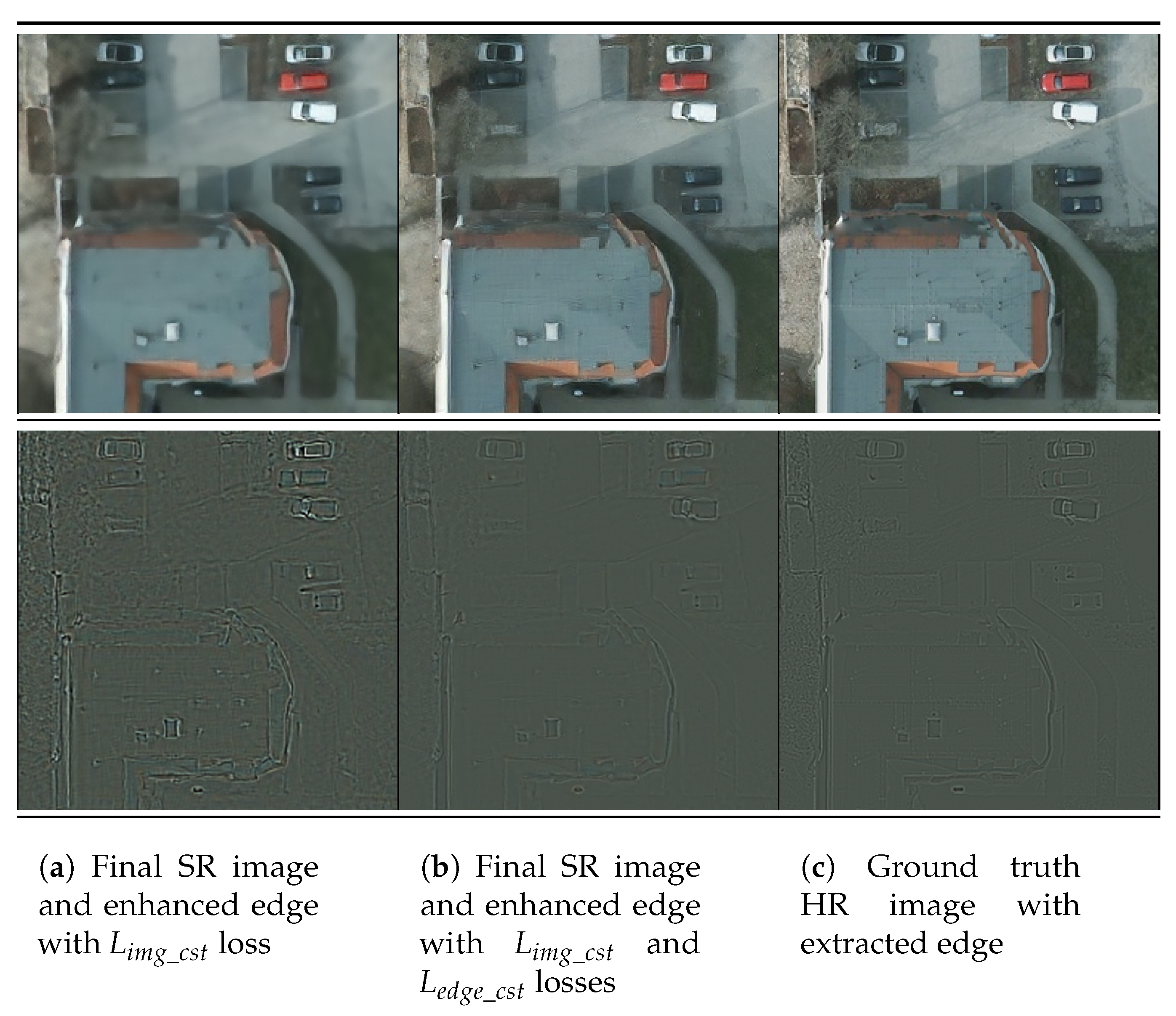
4.3.8. Effects of Edge Consistency Loss ()
5. Discussion
6. Conclusions
Author Contributions
Funding
Acknowledgments
Conflicts of Interest
Abbreviations
| SRCNN | Single image Super-Resolution Convolutional Neural Network |
| VDSR | Very Deep Convolutional Networks |
| GAN | Generative Adversarial Network |
| SRGAN | Super-Resolution Generative Adversarial Network |
| ESRGAN | Enhanced Super-Resolution Generative Adversarial Network |
| EEGAN | Edge-Enhanced Generative Adversarial Network |
| EESRGAN | Edge-Enhanced Super-Resolution Generative Adversarial Network |
| RRDB | Residual-in-Residual Dense Blocks |
| EEN | Edge-Enhancement Network |
| SSD | Single-Shot MultiBox Detector |
| YOLO | You Only Look Once |
| CNN | Convolutional Neural Network |
| R-CNN | Region-based Convolutional Neural Network |
| FRCNN | Faster Region-based Convolutional Neural Network |
| VGG | Visual Geometry Group |
| BN | Batch Normalization |
| MSCOCO | Microsoft Common Objects in Context |
| OGST | Oil and Gas Storage Tank |
| COWC | Car Overhead With Context |
| GSD | Ground Sampling Distance |
| G | Generator |
| D | Discriminator |
| ISR | Intermediate Super-Resolution |
| SR | Super-Resolution |
| HR | High-Resolution |
| LR | Low-Resoluton |
| GT | Ground Truth |
| FPN | Feature Pyramid Network |
| RPN | Region Proposal Network |
| AER | Alberta Energy Regulator |
| AGS | Alberta Geological Survey |
| AP | Average Precision |
| IoU | Intersection over Union |
| TP | True Positive |
| FP | False Positive |
| FN | False Negative |
References
- Colomina, I.; Molina, P. Unmanned aerial systems for photogrammetry and remote sensing: A review. ISPRS J. Photogramm. Remote Sens. 2014, 92, 79–97. [Google Scholar] [CrossRef]
- Zhang, F.; Du, B.; Zhang, L.; Xu, M. Weakly supervised learning based on coupled convolutional neural networks for aircraft detection. IEEE Trans. Geosci. Remote Sens. 2016, 54, 5553–5563. [Google Scholar] [CrossRef]
- Fromm, M.; Schubert, M.; Castilla, G.; Linke, J.; McDermid, G. Automated Detection of Conifer Seedlings in Drone Imagery Using Convolutional Neural Networks. Remote Sens. 2019, 11, 2585. [Google Scholar] [CrossRef]
- Pang, J.; Li, C.; Shi, J.; Xu, Z.; Feng, H. R2 -CNN: Fast Tiny Object Detection in Large-Scale Remote Sensing Images. IEEE Trans. Geosci. Remote Sens. 2019, 57, 5512–5524. [Google Scholar] [CrossRef]
- Shermeyer, J.; Van Etten, A. The effects of super-resolution on object detection performance in satellite imagery. In Proceedings of the IEEE Conference on Computer Vision and Pattern Recognition Workshops (CVPR 2019), Long Beach, CA, USA, 16–20 June 2019; pp. 1–10. [Google Scholar]
- Russakovsky, O.; Deng, J.; Su, H.; Krause, J.; Satheesh, S.; Ma, S.; Huang, Z.; Karpathy, A.; Khosla, A.; Bernstein, M.; et al. ImageNet Large Scale Visual Recognition Challenge. Int. J. Comput. Vis. 2015, 115, 211–252. [Google Scholar] [CrossRef]
- Lin, T.Y.; Maire, M.; Belongie, S.; Hays, J.; Perona, P.; Ramanan, D.; Dollár, P.; Zitnick, C.L. Microsoft coco: Common objects in context. In European Conference on Computer Vision; Springer: Berlin/Heidelberg, Germany, 2014; pp. 740–755. [Google Scholar]
- Ren, S.; He, K.; Girshick, R.; Sun, J. Faster R-CNN: Towards Real-Time Object Detection with Region Proposal Networks. IEEE Trans. Pattern Anal. Mach. Intell. 2017, 39, 1137–1149. [Google Scholar] [CrossRef] [PubMed]
- Lin, T.Y.; Goyal, P.; Girshick, R.; He, K.; Dollar, P. Focal Loss for Dense Object Detection. In Proceedings of the 2017 IEEE International Conference on Computer Vision (ICCV), Venice, Italy, 22–29 October 2017. [Google Scholar]
- Liu, W.; Anguelov, D.; Erhan, D.; Szegedy, C.; Reed, S.; Fu, C.Y.; Berg, A.C. SSD: Single Shot MultiBox Detector. In European Conference on Computer Vision; Lecture Notes in Computer Science; Springer: Cham, Switzerland, 2016; pp. 21–37. [Google Scholar] [CrossRef]
- Redmon, J.; Divvala, S.; Girshick, R.; Farhadi, A. You Only Look Once: Unified, Real-Time Object Detection. In Proceedings of the 2016 IEEE Conference on Computer Vision and Pattern Recognition (CVPR), Las Vegas, NV, USA, 26 June–1 July 2016. [Google Scholar] [CrossRef]
- Ji, H.; Gao, Z.; Mei, T.; Ramesh, B. Vehicle Detection in Remote Sensing Images Leveraging on Simultaneous Super-Resolution. In IEEE Geoscience and Remote Sensing Letters; IEEE-INST ELECTRICAL ELECTRONICS ENGINEERS INC.: New York, NY, USA, 2019; pp. 1–5. [Google Scholar] [CrossRef]
- Tayara, H.; Soo, K.G.; Chong, K.T. Vehicle detection and counting in high-resolution aerial images using convolutional regression neural network. IEEE Access 2017, 6, 2220–2230. [Google Scholar] [CrossRef]
- Yu, X.; Shi, Z. Vehicle detection in remote sensing imagery based on salient information and local shape feature. Opt.-Int. J. Light Electron. Opt. 2015, 126, 2485–2490. [Google Scholar] [CrossRef]
- Stankov, K.; He, D.C. Detection of buildings in multispectral very high spatial resolution images using the percentage occupancy hit-or-miss transform. IEEE J. Sel. Top. Appl. Earth Obs. Remote Sens. 2014, 7, 4069–4080. [Google Scholar] [CrossRef]
- Ok, A.O.; Başeski, E. Circular oil tank detection from panchromatic satellite images: A new automated approach. IEEE Geosci. Remote Sens. Lett. 2015, 12, 1347–1351. [Google Scholar] [CrossRef]
- Dong, C.; Loy, C.C.; He, K.; Tang, X. Image Super-Resolution Using Deep Convolutional Networks. IEEE Trans. Pattern Anal. Mach. Intell. 2016, 38, 295–307. [Google Scholar] [CrossRef] [PubMed]
- Kim, J.; Lee, J.K.; Lee, K.M. Accurate Image Super-Resolution Using Very Deep Convolutional Networks. In Proceedings of the 2016 IEEE Conference on Computer Vision and Pattern Recognition (CVPR), Las Vegas, NV, USA, 26 June–1 July 2016. [Google Scholar] [CrossRef]
- Goodfellow, I.; Pouget-Abadie, J.; Mirza, M.; Xu, B.; Warde-Farley, D.; Ozair, S.; Courville, A.; Bengio, Y. Generative adversarial nets. In Proceedings of the Advances in Neural Information Processing Systems, Montreal, QC, Canada, 8–13 December 2014; pp. 2672–2680. [Google Scholar]
- Ledig, C.; Theis, L.; Huszar, F.; Caballero, J.; Cunningham, A.; Acosta, A.; Aitken, A.; Tejani, A.; Totz, J.; Wang, Z.; et al. Photo-Realistic Single Image Super-Resolution Using a Generative Adversarial Network. In Proceedings of the 2017 IEEE Conference on Computer Vision and Pattern Recognition (CVPR), Honolulu, HI, USA, 21–26 July 2017. [Google Scholar] [CrossRef]
- Wang, X.; Yu, K.; Wu, S.; Gu, J.; Liu, Y.; Dong, C.; Qiao, Y.; Loy, C.C. ESRGAN: Enhanced Super-Resolution Generative Adversarial Networks. In Proceedings of the Computer Vision—ECCV 2018 Workshops, Munich, Germany, 8–14 September 2018; pp. 63–79. [Google Scholar] [CrossRef]
- Jiang, K.; Wang, Z.; Yi, P.; Wang, G.; Lu, T.; Jiang, J. Edge-Enhanced GAN for Remote Sensing Image Superresolution. IEEE Trans. Geosci. Remote Sens. 2019, 57, 5799–5812. [Google Scholar] [CrossRef]
- Jiang, J.; Ma, J.; Wang, Z.; Chen, C.; Liu, X. Hyperspectral Image Classification in the Presence of Noisy Labels. IEEE Trans. Geosci. Remote Sens. 2019, 57, 851–865. [Google Scholar] [CrossRef]
- Tong, F.; Tong, H.; Jiang, J.; Zhang, Y. Multiscale union regions adaptive sparse representation for hyperspectral image classification. Remote Sens. 2017, 9, 872. [Google Scholar] [CrossRef]
- Zhan, C.; Duan, X.; Xu, S.; Song, Z.; Luo, M. An improved moving object detection algorithm based on frame difference and edge detection. In Proceedings of the Fourth International Conference on Image and Graphics (ICIG 2007), Sichuan, China, 22–24 August 2007; pp. 519–523. [Google Scholar]
- Mao, Q.; Wang, S.; Wang, S.; Zhang, X.; Ma, S. Enhanced image decoding via edge-preserving generative adversarial networks. In Proceedings of the 2018 IEEE International Conference on Multimedia and Expo (ICME), San Diego, CA, USA, 23–27 July 2018; pp. 1–6. [Google Scholar]
- Yang, W.; Feng, J.; Yang, J.; Zhao, F.; Liu, J.; Guo, Z.; Yan, S. Deep Edge Guided Recurrent Residual Learning for Image Super-Resolution. IEEE Trans. Image Process. 2017, 26, 5895–5907. [Google Scholar] [CrossRef] [PubMed]
- Kamgar-Parsi, B.; Kamgar-Parsi, B.; Rosenfeld, A. Optimally isotropic Laplacian operator. IEEE Trans. Image Process. 1999, 8, 1467–1472. [Google Scholar] [CrossRef]
- Landsat 8. Available online: https://www.usgs.gov/land-resources/nli/landsat/landsat-8 (accessed on 11 February 2020).
- Sentinel-2. Available online: http://www.esa.int/Applications/Observing_the_Earth/Copernicus/Sentinel-2 (accessed on 11 February 2020).
- Mundhenk, T.N.; Konjevod, G.; Sakla, W.A.; Boakye, K. A large contextual dataset for classification, detection and counting of cars with deep learning. In European Conference on Computer Vision; Springer: Cham, Switzerland, 2016; pp. 785–800. [Google Scholar]
- Rabbi, J.; Chowdhury, S.; Chao, D. Oil and Gas Tank Dataset. In Mendeley Data, V3; 2020; Available online: https://data.mendeley.com/datasets/bkxj8z84m9/3 (accessed on 30 April 2020). [CrossRef]
- Jolicoeur-Martineau, A. The Relativistic Discriminator: A Key Element Missing from Standard GAN. arXiv 2018, arXiv:1807.00734. [Google Scholar]
- Charbonnier, P.; Blanc-Féraud, L.; Aubert, G.; Barlaud, M. Two deterministic half-quadratic regularization algorithms for computed imaging. Proc. Int. Conf. Image Process. 1994, 2, 168–172. [Google Scholar]
- Alberta Energy Regulator. Available online: https://www.aer.ca (accessed on 5 February 2020).
- Tai, Y.; Yang, J.; Liu, X.; Xu, C. MemNet: A Persistent Memory Network for Image Restoration. In Proceedings of the 2017 IEEE International Conference on Computer Vision (ICCV), Venice, Italy, 22–29 October 2017. [Google Scholar] [CrossRef]
- Zhang, Y.; Tian, Y.; Kong, Y.; Zhong, B.; Fu, Y. Residual Dense Network for Image Super-Resolution. In Proceedings of the 2018 IEEE/CVF Conference on Computer Vision and Pattern Recognition, Salt Lake City, UT, USA, 18–23 June 2018. [Google Scholar] [CrossRef]
- He, K.; Zhang, X.; Ren, S.; Sun, J. Delving Deep into Rectifiers: Surpassing Human-Level Performance on ImageNet Classification. In Proceedings of the 2015 IEEE International Conference on Computer Vision (ICCV), Santiago, Chile, 7–13 December 2015. [Google Scholar] [CrossRef]
- Lim, B.; Son, S.; Kim, H.; Nah, S.; Lee, K.M. Enhanced Deep Residual Networks for Single Image Super-Resolution. In Proceedings of the 2017 IEEE Conference on Computer Vision and Pattern Recognition Workshops (CVPRW), Honolulu, HI, USA, 21–26 July 2017. [Google Scholar] [CrossRef]
- Liebel, L.; Körner, M. Single-image super resolution for multispectral remote sensing data using convolutional neural networks. ISPRS Int. Arch. Photogramm. Remote Sens. Spat. Inf. Sci. 2016, 41, 883–890. [Google Scholar] [CrossRef]
- Tayara, H.; Chong, K. Object detection in very high-resolution aerial images using one-stage densely connected feature pyramid network. Sensors 2018, 18, 3341. [Google Scholar] [CrossRef]
- Girshick, R.; Donahue, J.; Darrell, T.; Malik, J. Rich Feature Hierarchies for Accurate Object Detection and Semantic Segmentation. In Proceedings of the 2014 IEEE Conference on Computer Vision and Pattern Recognition, Columbus, OH, USA, 24–27 June 2014. [Google Scholar] [CrossRef]
- Girshick, R. Fast R-CNN. In Proceedings of the 2015 IEEE International Conference on Computer Vision (ICCV), Santiago, Chile, 7–13 December 2015. [Google Scholar] [CrossRef]
- Li, Q.; Mou, L.; Xu, Q.; Zhang, Y.; Zhu, X.X. R3-Net: A Deep Network for Multioriented Vehicle Detection in Aerial Images and Videos. IEEE Trans. Geosci. Remote Sens. 2019, 57, 5028–5042. [Google Scholar] [CrossRef]
- Ammour, N.; Alhichri, H.; Bazi, Y.; Benjdira, B.; Alajlan, N.; Zuair, M. Deep learning approach for car detection in UAV imagery. Remote Sens. 2017, 9, 312. [Google Scholar] [CrossRef]
- Ren, Y.; Zhu, C.; Xiao, S. Small object detection in optical remote sensing images via modified faster R-CNN. Appl. Sci. 2018, 8, 813. [Google Scholar] [CrossRef]
- Tang, T.; Zhou, S.; Deng, Z.; Zou, H.; Lei, L. Vehicle detection in aerial images based on region convolutional neural networks and hard negative example mining. Sensors 2017, 17, 336. [Google Scholar] [CrossRef] [PubMed]
- Chen, Z.; Zhang, T.; Ouyang, C. End-to-end airplane detection using transfer learning in remote sensing images. Remote Sens. 2018, 10, 139. [Google Scholar] [CrossRef]
- Radovic, M.; Adarkwa, O.; Wang, Q. Object recognition in aerial images using convolutional neural networks. J. Imaging 2017, 3, 21. [Google Scholar] [CrossRef]
- Li, W.; Fu, H.; Yu, L.; Cracknell, A. Deep learning based oil palm tree detection and counting for high-resolution remote sensing images. Remote Sens. 2017, 9, 22. [Google Scholar] [CrossRef]
- Lin, T.Y.; Dollar, P.; Girshick, R.; He, K.; Hariharan, B.; Belongie, S. Feature Pyramid Networks for Object Detection. In Proceedings of the 2017 IEEE Conference on Computer Vision and Pattern Recognition (CVPR), Honolulu, HI, USA, 21–26 July 2017. [Google Scholar] [CrossRef]
- Liu, S.; Huang, D. Receptive field block net for accurate and fast object detection. In Proceedings of the European Conference on Computer Vision (ECCV), Munich, Germany, 8–14 September 2018; pp. 385–400. [Google Scholar]
- Zhang, S.; Wen, L.; Bian, X.; Lei, Z.; Li, S.Z. Single-shot refinement neural network for object detection. In Proceedings of the IEEE conference on Computer Vision and Pattern Recognition, Salt Lake City, UT, USA, 18–22 June 2018; pp. 4203–4212. [Google Scholar]
- Li, Z.; Zhou, F. FSSD: Feature fusion single shot multibox detector. arXiv 2017, arXiv:1712.00960. [Google Scholar]
- Zhu, R.; Zhang, S.; Wang, X.; Wen, L.; Shi, H.; Bo, L.; Mei, T. ScratchDet: Training single-shot object detectors from scratch. In Proceedings of the IEEE Conference on Computer Vision and Pattern Recognition, Long Beach, CA, USA, 15–20 June 2019; pp. 2268–2277. [Google Scholar]
- Yang, X.; Sun, H.; Fu, K.; Yang, J.; Sun, X.; Yan, M.; Guo, Z. Automatic ship detection in remote sensing images from google earth of complex scenes based on multiscale rotation dense feature pyramid networks. Remote Sens. 2018, 10, 132. [Google Scholar] [CrossRef]
- Zhao, Z.Q.; Zheng, P.; Xu, S.T.; Wu, X. Object detection with deep learning: A review. IEEE Trans. Neural Netw. Learn. Syst. 2019, 30, 3212–3232. [Google Scholar] [CrossRef]
- Li, K.; Wan, G.; Cheng, G.; Meng, L.; Han, J. Object detection in optical remote sensing images: A survey and a new benchmark. ISPRS J. Photogramm. Remote Sens. 2020, 159, 296–307. [Google Scholar] [CrossRef]
- Bai, Y.; Zhang, Y.; Ding, M.; Ghanem, B. Sod-mtgan: Small object detection via multi-task generative adversarial network. In Proceedings of the European Conference on Computer Vision (ECCV), Munich, Germany, 8–14 September 2018; pp. 206–221. [Google Scholar]
- Haris, M.; Shakhnarovich, G.; Ukita, N. Task-driven super resolution: Object detection in low-resolution images. arXiv 2018, arXiv:1803.11316. [Google Scholar]
- Zhu, J.Y.; Park, T.; Isola, P.; Efros, A.A. Unpaired image-to-image translation using cycle-consistent adversarial networks. In Proceedings of the IEEE International Conference on Computer Vision, Venice, Italy, 22–29 October 2017; pp. 2223–2232. [Google Scholar]
- Simonyan, K.; Zisserman, A. Very Deep Convolutional Networks for Large-Scale Image Recognition. arXiv 2014, arXiv:1409.1556. [Google Scholar]
- Lai, W.S.; Huang, J.B.; Ahuja, N.; Yang, M.H. Deep Laplacian Pyramid Networks for Fast and Accurate Super-Resolution. In Proceedings of the 2017 IEEE Conference on Computer Vision and Pattern Recognition (CVPR), Honolulu, HI, USA, 21–26 July 2017. [Google Scholar] [CrossRef]
- Kingma, D.P.; Ba, J. Adam: A method for stochastic optimization. arXiv 2014, arXiv:1412.6980. [Google Scholar]
- Paszke, A.; Gross, S.; Massa, F.; Lerer, A.; Bradbury, J.; Chanan, G.; Killeen, T.; Lin, Z.; Gimelshein, N.; Antiga, L.; et al. PyTorch: An Imperative Style, High-Performance Deep Learning Library. In Advances in Neural Information Processing Systems 32; Wallach, H., Larochelle, H., Beygelzimer, A., d’Alché Buc, F., Fox, E., Garnett, R., Eds.; Curran Associates, Inc.: New York, NY, USA, 2019; pp. 8024–8035. [Google Scholar]
- Rabbi, J. Edge Enhanced GAN with Faster RCNN for End-to-End Object Detection from Remote Sensing Imagery. 2020. Available online: https://github.com/Jakaria08/Filter_Enhance_Detect (accessed on 28 April 2020).
- Alberta Geological Survey. Available online: https://ags.aer.ca (accessed on 5 February 2020).
- Chowdhury, S.; Chao, D.K.; Shipman, T.C.; Wulder, M.A. Utilization of Landsat data to quantify land-use and land-cover changes related to oil and gas activities in West-Central Alberta from 2005 to 2013. GISci. Remote Sens. 2017, 54, 700–720. [Google Scholar] [CrossRef]
- Bing Map. Available online: https://www.bing.com/maps (accessed on 5 February 2020).
- Bulat, A.; Yang, J.; Tzimiropoulos, G. To learn image super-resolution, use a gan to learn how to do image degradation first. In Proceedings of the European Conference on Computer Vision (ECCV), Munich, Germany, 8–14 September 2018; pp. 185–200. [Google Scholar]


| Model | Training Image Resolution-Test Image Resolution | COWC Dataset (Test Results) (AP at IoU = 0.5:0.95) (Single Class-15 cm) | OGST Dataset (Test Results) (AP at IoU = 0.5:0.95) (Single Class-30 cm) |
|---|---|---|---|
| SSD | LR-LR | 61.9% | 76.5% |
| HR-LR | 58% | 75.3% | |
| FRCNN | LR-LR | 64% | 77.3% |
| HR-LR | 59.7% | 75% | |
| SSD-RFB | LR-LR | 63.1% | 76.7% |
| SSD | HR-HR | 94.1% | 82.5% |
| FRCNN | HR-HR | 98% | 84.9% |
| Model | Training Image Resolution-Test Image Resolution | COWC Dataset (Test Results) (AP at IoU = 0.5:0.95) (Single Class-15 cm) | OGST Dataset (Test Results) (AP at IoU = 0.5:0.95) (Single Class-30 cm) |
|---|---|---|---|
| Bicubic + SSD | SR-SR | 72.1% | 77.6% |
| HR-SR | 58.3% | 76% | |
| Bicubic + FRCNN | SR-SR | 76.8% | 78.5% |
| HR-SR | 61.5% | 77.1% | |
| EESRGAN + SSD | SR-SR | 86% | 80.2% |
| HR-SR | 83.1% | 79.4% | |
| EESRGAN + FRCNN | SR-SR | 93.6% | 81.4% |
| HR-SR | 92.9% | 80.6% | |
| ESRGAN + SSD | SR-SR | 85.8% | 80.2% |
| HR-SR | 82.5% | 78.9% | |
| ESRGAN + FRCNN | SR-SR | 92.5% | 81.1% |
| HR-SR | 91.8% | 79.3% | |
| EEGAN + SSD | SR-SR | 86.1% | 79.1% |
| HR-SR | 83.3% | 77.5% | |
| EEGAN + FRCNN | SR-SR | 92% | 79.9% |
| HR-SR | 91.1% | 77.9% |
| Model | Training Image Resolution-Test Image Resolution | COWC Dataset (Test Results) (AP at IoU = 0.5:0.95) (Single Class-15 cm) | OGST Dataset (Test Results) (AP at IoU = 0.5:0.95) (Single Class-30 cm) |
|---|---|---|---|
| EESRGAN + SSD | SR-SR | 89.3% | 81.8% |
| EESRGAN + FRCNN | SR-SR | 95.5% | 83.2% |
| ESRGAN + SSD | SR-SR | 88.5% | 81.1% |
| ESRGAN + FRCNN | SR-SR | 93.6% | 82% |
| EEGAN + SSD | SR-SR | 88.1% | 80.8% |
| EEGAN + FRCNN | SR-SR | 93.1% | 81.3% |
© 2020 by the authors. Licensee MDPI, Basel, Switzerland. This article is an open access article distributed under the terms and conditions of the Creative Commons Attribution (CC BY) license (http://creativecommons.org/licenses/by/4.0/).
Share and Cite
Rabbi, J.; Ray, N.; Schubert, M.; Chowdhury, S.; Chao, D. Small-Object Detection in Remote Sensing Images with End-to-End Edge-Enhanced GAN and Object Detector Network. Remote Sens. 2020, 12, 1432. https://doi.org/10.3390/rs12091432
Rabbi J, Ray N, Schubert M, Chowdhury S, Chao D. Small-Object Detection in Remote Sensing Images with End-to-End Edge-Enhanced GAN and Object Detector Network. Remote Sensing. 2020; 12(9):1432. https://doi.org/10.3390/rs12091432
Chicago/Turabian StyleRabbi, Jakaria, Nilanjan Ray, Matthias Schubert, Subir Chowdhury, and Dennis Chao. 2020. "Small-Object Detection in Remote Sensing Images with End-to-End Edge-Enhanced GAN and Object Detector Network" Remote Sensing 12, no. 9: 1432. https://doi.org/10.3390/rs12091432
APA StyleRabbi, J., Ray, N., Schubert, M., Chowdhury, S., & Chao, D. (2020). Small-Object Detection in Remote Sensing Images with End-to-End Edge-Enhanced GAN and Object Detector Network. Remote Sensing, 12(9), 1432. https://doi.org/10.3390/rs12091432