Deep Open-Set Domain Adaptation for Cross-Scene Classification based on Adversarial Learning and Pareto Ranking

Abstract

Most of the existing domain adaptation (DA) methods proposed in the context of remote sensing imagery assume the presence of the same land-cover classes in the source and target domains. Yet, this assumption is not always realistic in practice as the target domain may contain additional classes unknown to the source leading to the so-called open set DA. Under this challenging setting, the problem turns to reducing the distribution discrepancy between the shared classes in both domains besides the detection of the unknown class samples in the target domain. To deal with the openset problem, we propose an approach based on adversarial learning and pareto-based ranking. In particular, the method leverages the distribution discrepancy between the source and target domains using min-max entropy optimization. During the alignment process, it identifies candidate samples of the unknown class from the target domain through a pareto-based ranking scheme that uses ambiguity criteria based on entropy and the distance to source class prototype. Promising results using two cross-domain datasets that consist of very high resolution and extremely high resolution images, show the effectiveness of the proposed method.

1. Introduction

Scene classification is the process of automatically assigning an image to a class label that describes the image correctly. In the field of remote sensing, scene classification gained a lot of attention and several methods were introduced in this field such as bag of word model [1], compressive sensing [2], sparse representation [3], and lately deep learning [4]. To classify a scene correctly, effective features are extracted from a given image, then classified by a classifier to the correct label. Early studies of remote sensing scene classification were based on handcrafted features [1,5,6]. In this context, deep learning techniques showed to be very efficient in terms compared to standard solutions based on handcrafted features. Convolutional neural networks (CNN) are considered the most common deep learning techniques for learning visual features and they are widely used to classify remote sensing images [7,8,9]. Several approaches were built around these methods to boost the classification results such as integrating local and global features [10,11,12], recurrent neural networks (RNNs) [13,14], and generative adversarial networks (GANs) [15].

The number of remote sensing images has been steadily increasing over the years. These images are collected using different sensors mounted on satellites or airborne platforms. The type of the sensor results in different image resolutions: spatial, spectral, and temporal resolution. This leads to huge number of images with different spatial and spectral resolutions [16]. In many real-world applications, the training data used to learn a model may have different distributions from the data used for testing, when images are acquired over different locations and with different sensors. For such purpose, it becomes necessary to reduce the distribution gap between the source and target domains to obtain acceptable classification results [17]. The main goal of domain adaptation is to learn a classification model from a labeled source domain and apply this model to classify an unlabeled target domain. Several methods have been introduced related to domain adaptation in the field of remote sensing [18,19,20,21].

The above methods assume that the sample belongs to one of a fixed number of known classes. This is called a closed set domain adaptation, where the source and target domains have shared classes only. This assumption is violated in many cases. In fact, many real applications follow an open set environment, where some test samples belong to classes that are unknown during training [22]. These samples are supposed to be classified as unknown, instead of being classified to one of the shared classes. Classifying the unknown image to one of the shared classes leads to negative transfer. Figure 1 shows the difference between open and closed set classification. This problem is known in the community of machine learning as open set domain adaptation. Thus, in an open set domain adaptation one has to learn robust feature representations for the source labeled data, reduce the data-shift problem between the source and target distributions, and detect the presence of new classes in the target domain.

Figure 1. (a) Closed set domain adaptation: source and target domains share the same classes. (b) Open set domain adaptation: target domain contains unknown classes (in the grey boxes).

Open set classification is a new research area in the remote sensing field. Few works have introduced the problem of open set. Anne Pavy and Edmund Zelnio [23] introduced a method to classify Synthetic Aperture Radar (SAR) images in the test samples that are in the training samples and reject those not in the training set as unknown. The method uses a CNN as a feature extractor and SVM for classification and rejection of unknowns. Wang et al. [24] addressed the open set problem in high range resolution profile (HRRP) recognition. The method is based on random forest (RF) and extreme value theory, the RF is used to extract the high-level features of the input image, then used as input to the open set module. The two approaches use a single domain for training and testing.

To the best of our knowledge, no previous works have addressed the open-set domain adaptation problem for remote sensing images where the source domain is different from the target domain. To address this issue, the method we propose is based on adversarial learning and pareto-based ranking. In particular, the method leverages the distribution discrepancy between the source and target domain using min-max entropy optimization. During the alignment process, it identifies candidate samples of the unknown class from the target domain through a pareto-based ranking scheme that uses ambiguity criteria based on entropy and the distance to source class porotypes.

2. Related Work on Open Set Classification

Open set classification is a more challenging and more realistic approach, thus it has gained a lot of attention by researchers lately and many works are done in this field. Early research on open set classification depended on traditional machine learning techniques, such as support vector machines (SVMs). Scheirer et al. [25] first proposed 1-vs-Set method which used a binary SVM classifier to detect unknown classes. The method introduced a new open set margin to decrease the region of the known class for each binary SVM. Jain et al. [26] invoked the extreme value theory (EVT) to present a multi-class open set classifier to reject the unknowns. The authors introduced the Pi-SVM algorithm to estimate the un-normalized posterior class inclusion likelihood. The probabilistic open set SVM (POS-SVM) classifier proposed by Scherreik et al. [27] empirically determines the unique reject threshold for each known class. Sparse representation techniques were used in open set classification, where the sparse representation based classifier (SRC) [28] looks for the sparest possible representation of the test sample to correctly classify the sample [29]. Bendale and Boult [30] presented the nearest non-outlier (NNO) method to actively detect and learn new classes, taking into account the open space risk and metric learning.

Deep neural networks (DNNs) were very interesting in several tasks lately, including open set classification. Bendale and Boult [31] first introduced OpenMax model, which is a DNN to perform open set classification. The OpenMax layer replaced the softmax layer in a CNN to check if a given sample belongs to an unknown class. Hassen and Chan [32] presented a method to solve the open set problem, by keeping instances belonging to the same class near each other, and instances that belong to different or unknown classes farther apart. Shu et al. [33] proposed deep open classification (DOC) for open set classification, that builds a multi-class classifier which used instead of the last softmax layer a 1-vs-rest layer of sigmoids to make the open space risk as small as possible. Later, Shu et al. [34] presented a model for discovering unknown classes that combines two neural networks: open classification network (OCN) for seen classification and unseen class rejection, and a pairwise classification network (PCN) which learns a binary classifier to predict if two samples come from the same class or different classes.

In the last years generative adversarial networks (GANs) [35] were introduced to the field of open set classification. Ge et al. [36] presented the Generative OpenMax (G-OpenMax) method. The algorithm adapts OpenMax to generative adversarial networks for open set classification. The GAN trained the network by generating unknown samples, then combined it with an OpenMax layer to reject samples belonging to the unknown class. Neal et al. [37] proposed another GAN-based algorithm to generate counterfactual images that do not belong to any class; instead are unknown, which are used to train a classifier to correctly classify unknown images. Yu et al. [38] also proposed a GAN that generated negative samples for known classes to train the classifier to distinguish between known and unknown samples.

Most of the previous studies mentioned in the literature of scene classification assume that one domain is used for both training and testing. This assumption is not always satisfied, due to the fact that some domains have images that are labeled, on the other hand many new domains have shortage in labeled images. It will be time-consuming and expensive to generate and collect large datasets of labeled images. One suggestion to solve this issue is to use labeled images from one domain as training data for different domains. Domain adaptation is one part of transfer learning where transfer of knowledge occurs between two domains, source and target. Domain adaptation approaches differ from each other in the percentage of labeled images in the target domain. Some works have been done in the field of open set domain adaptation. First, Busto et al. [22] introduced open set domain adaptation in their work, by allowing the target domain to have samples of classes not belonging to the source domain and vice versa. The classes not shared or uncommon are joined as a negative class called “unknown”. The goal was to correctly classify target samples to the correct class if shared between source and target, and classify samples to unknown if not shared between domains. Saito et al. [39] proposed a method where unknown samples appear only in the target domain, which is more challenging. The proposed approach introduced adversarial learning where the generator can separate target samples to known and unknown classes. The generator can decide to reject or accept the target image. If accepted, it is classified to one of the classes in the source domain. If rejected it is classified as unknown.

Cao et al. [40] introduced a new partial domain adaptation method, they assumed that the target dataset contained classes that are a subset of the source dataset classes. This makes the domain adaptation problem more challenging due to the extra source classes, which could result in negative transfer problems. The authors used a multi-discriminator domain adversarial network, where each discriminator has the responsibility of matching the source and target domain data after filtering unknown source classes. Zhang et al. [41] also introduced the problem of transferring from big source to target domain with subset classes. The method requires only two domain classifiers instead of multiple classifiers one for each domain as shown by the previous method. Furthermore, Baktashmotlagh et al. [42] proposed an approach to factorize the data into shared and private sub-spaces. Source and target samples coming from the same, known classes can be represented by a shared subspace, while target samples from unknown classes were modeled with a private subspace.

Lian et al. [43] proposed Known-class Aware Self-Ensemble (KASE) that was able to reject unknown classes. The model consists of two modules to effectively identify known and unknown classes and perform domain adaptation based on the likeliness of target images belonging to known classes. Lui et al. [44] presented Separate to Adapt (STA), a method to separate known from unknown samples in an advanced way. The method works in two steps: first a classifier was trained to measure the similarity between target samples and every source class with source samples. Then, high and low values of similarity were selected to be known and unknown classes. These values were used to train a classifier to correctly classify target images. Tan et al. [45] proposed a weakly supervised method, where the source and target domains had some labeled images. The two domains learn from each other through the few labeled images to correctly classify the unlabeled images in both domains. The method aligns the source and target domains in a collaborative way and then maximizes the margin for the shared and unshared classes.

In the contest of remote sensing, open set domain adaptation is a new research field and no previous work was achieved.

3. Description of the Proposed Method

Assume a labeled source domain $D_s={\left\{\left(X_i^{\left(s\right)},y_i^{\left(s\right)}\right)\right\}}_{i=1}^{n_s}$ composed of $X_i^{\left(s\right)}$ images and their corresponding class labels $y_i^{\left(s\right)}\in \left\{1,2,\dots ,K\right\}$, where $n_s$ is the number of images and $K$ is the number of classes. Additionally, we assume an unlabeled target domain $D_t={\left\{\left(X_j^{\left(t\right)}\right)\right\}}_{j=1}^{n_t}$ with $n_t$ unlabeled images. In an open set setting, the target domain contains $K+1$ classes, where $K$ classes are shared with the source domain, and an addition unknown class (can be many unknown classes but grouped in one class). The objective of this work is twofold: (1) reduce the distribution discrepancy between the source and target domains, and (2) detect the presence of the unknown class in the target domain. Figure 2 shows the overall description of the proposed adversarial learning method, which relies on the idea of min-max entropy for carrying out the domain adaptation and uses an unknown class detector based on pareto ranking.

Figure 2. Proposed open-set domain adaptation method.

3.1. Network Architecture

Our model uses EfficientNet-B3 network [46] from Google as a feature extractor although other networks could be used as well since the method is independent of the pre-trained CNN. The choice of this network is motivated by its ability to generate high classification accuracies but with reduced parameters compared to other architectures. EfficientNets are based on the concept of scaling up CNNs by means of a compound coefficient, which jointly integrates the width, depth, and resolution. Basically, each dimension is scaled in a balanced way using a set of scaling coefficients. We truncate this network by removing its original ImageNet-based softmax classification layer. For computation convenience, we set ${\left\{h_i^{\left(s\right)}\right\}}_{i=1}^{n_s}$ and ${\left\{h_j^{\left(t\right)}\right\}}_{j=1}^{n_t}$ as the feature representations for both source and target data obtained at the output of this trimmed CNN (each feature is a vector of dimension 1536). These features are further subject to dimensionality reduction via a fully-connected layer $F$ acting as a feature extractor yielding new feature representations ${\left\{z_i^{\left(s\right)}\right\}}_{i=1}^{n_s}$ and ${\left\{z_j^{\left(t\right)}\right\}}_{j=1}^{n_t}$ each of dimension 128. The output of $F$ is further normalized using $l_2$ normalization and fed as input to a decoder $D$ and similarity-based classifier $C$.

The decoder $D$ has the task to constrain the mapping spaces of $F$ with reconstruction ability to the original features provided by the pre-trained CNN in order to reduce the overlap between classes during adaptation. On the other side, the similarity classifier $C$ aims to assign images to the corresponding classes including the unknown one (identified using ranking criteria) by computing the similarity measure of their related representations to its weight $W=\left[{\mathrm{w}}_1,{\mathrm{w}}_2,\dots ,{\mathrm{w}}_{\mathrm{K}},{\mathrm{w}}_{\mathrm{K}+1}\right]$. These weights are viewed as estimated porotypes for the $K$-source classes and the unknown class with index $K+1$.

3.2. Adversarial Learning with Reconstruction Ability

We reduce the distribution discrepancy using an adversarial learning approach with reconstruction ability based on min-max entropy optimization [47]. To learn the weights of $\mathrm{F}$, $\mathrm{C}$, and $\mathrm{D}$ we use both labeled sources and unlabeled target samples. We learn the network to discriminate between the labeled classes in the source domain and the unknown class samples identified iteratively in the target domain (using the proposed pareto ranking scheme), while clustering the remaining target samples to the most suitable class prototypes. For such purpose, we jointly minimize the following loss functions:

$$\{\begin{array}{c}{L}_F=L_s\left(y^{\left(s\right)},{\widehat{y}}^{\left(s\right)}\right)+L_{K+1}\left(y^{\left(t\right)},{\widehat{y}}^{\left(t\right)}\right)+\lambda H\left({\widehat{y}}^{\left(t\right)}\right)\\ L_C=L_s\left(y^{\left(s\right)},{\widehat{y}}^{\left(s\right)}\right)+L_{K+1}\left(y^{\left(t\right)},{\widehat{y}}^{\left(t\right)}\right)-\lambda H\left({\widehat{y}}^{\left(t\right)}\right)\\ L_D=\frac{1}{n_s}{\displaystyle \sum }_{i=1}^{n_s}\Vert h_i^{\left(s\right)}-{\widehat{h}}_i^{\left(s\right)}\Vert {}^2+\frac{1}{n_t}{\displaystyle \sum }_{j=1}^{n_t}\Vert h_i^{\left(t\right)}-{\widehat{h}}_i^{\left(t\right)}\Vert {}^2\end{array}$$

(1)

where $\lambda$ is a regulalrization parameter which controls the contribution of the entropy to the total loss. $L_s$ is the categorical cross-entropy loss computed for the source domain:

$$L_s\left(y^{\left(s_k\right)},{\widehat{y}}^{\left(s_k\right)}\right)=-\frac{1}{n_{s_k}}{{\displaystyle \sum }}_{i=1}^{n_{s_k}}{{\displaystyle \sum }}_{k=1}^{K}1\left(k=y_{ik}^{\left(s_k\right)}\right)log\left({\widehat{y}}_{ik}^{\left(s_k\right)}\right)$$

(2)

${\mathrm{L}}_{K+1}$ is the cross-entropy loss computed for the samples iteratively identified as unknown class:

$$L_{K+1}\left(y^{\left(t_{K+1}\right)},{\widehat{y}}^{\left(t_{K+1}\right)}\right)=-\frac{1}{n_{t_{k+1}}}{{\displaystyle \sum }}_{j=1}^{n_{t_{K+1}}}{y}_j^{\left(t_{K+1}\right)}log\left({\widehat{y}}_j^{\left(t_{K+1}\right)}\right)$$

(3)

$\mathrm{H}\left({\hat{\mathrm{y}}}^{\left(\mathrm{t}\right)}\right)$ is the entropy computed for the samples of the target domain:

$$H\left({\widehat{y}}^{\left(t\right)}\right)=-\frac{1}{n_t}{{\displaystyle \sum }}_{i=1}^{n_t}{{\displaystyle \sum }}_{k=1}^{K+1}1\left(k={\widehat{y}}_{ik}^{\left(t\right)}\right)log\left({\widehat{y}}_{ik}^{\left(t\right)}\right)$$

(4)

and $L_D$ is the reconstruction loss.

From Equation (1), we observe that both $C$ and $F$ are used to learn discriminative features for the labeled samples. The classifier $C$ makes the target samples closer to the estimated prototypes by increasing the entropy. On the other side, the feature extractor $F$ tries to decrease it by assigning the target samples to the most suitable class prototype. On the other side, the decoder $D$ constrains the projection to the reconstruction space to control the overlap between the samples of the different classes. In the experiments, we will show that this learning mechanism allows to boost the classification accuracy of the target samples. In practice, we use a gradient reversal layer to flip the gradients of $H\left({\hat{\mathrm{y}}}^{\left({\mathrm{t}}_{\mathrm{k}}\right)}\right)$ between $\mathrm{C}$ and $\mathrm{F}.$ To this end, we use a gradient reverse layer [48] between $\mathrm{C}$ and $\mathrm{F}$ to flip the sign of gradient to simplify the training process. The gradient reverse layer aims to flip the sign of the input by multiplying it with a negative scalar in the backpropagation, while leaving it as it is in the forward propagation.

Pareto Ranking for Unknown Class Sample Selection

During the alignment of the source and target distributions, we strive for detecting the most $r<n_t$ ambiguous samples and assign a soft label to them (unknown class K+1). Indeed, the adversarial learning will push the target samples to the most suitable class prototypes in the source domain, while the most ambiguous ones will potentially indicate the presence of a new class. In this work, we use the entropy measure and the distance from the class prototypes as a possible solution for identifying these samples. In particular, we propose to rank the target samples using both measures.

An important aspect of pareto ranking is the concept of dominance widely applied in multi-objective optimization, which involves finding a set of pareto optimal solutions rather than a single one. This set of pareto optimal solutions contains solutions that cannot be improved on one of the objective functions without affecting the other functions. In our case, we formulate the problem as finding a sub-set $P$ from the unlabeled samples that maximizes the two objective functions $f_1$ and $f_2$, where

$$f_1^j=cosine\left(z_j^{\left(t\right)},{\overline{z}}_k^{\left(s\right)}\right), j=1,\dots ,n_t$$

(5)

$$f_2^j=-\frac{1}{n_t}{{\displaystyle \sum }}_{i=1}^{n_t}{{\displaystyle \sum }}_{k=1}^{K+1}1\left(k={\widehat{y}}_{ik}^{\left(t\right)}\right)log\left({\widehat{y}}_{ik}^{\left(t\right)}\right)$$

(6)

where $f_1^j$ is the cosine distance of the representation $z_j^{\left(t\right)}$ of the target sample $X_j^{\left(t\right)}$ with respect to the class porotypes ${\overline{z}}_k^{\left(s\right)}=\frac{1}{n_{sk}}{\displaystyle \sum }_{i=1}^{n_{sk}}{z}_{ik}$ of each source class, and $f_2^j$ is the cross-entropy loss computed for the samples of the target domain.

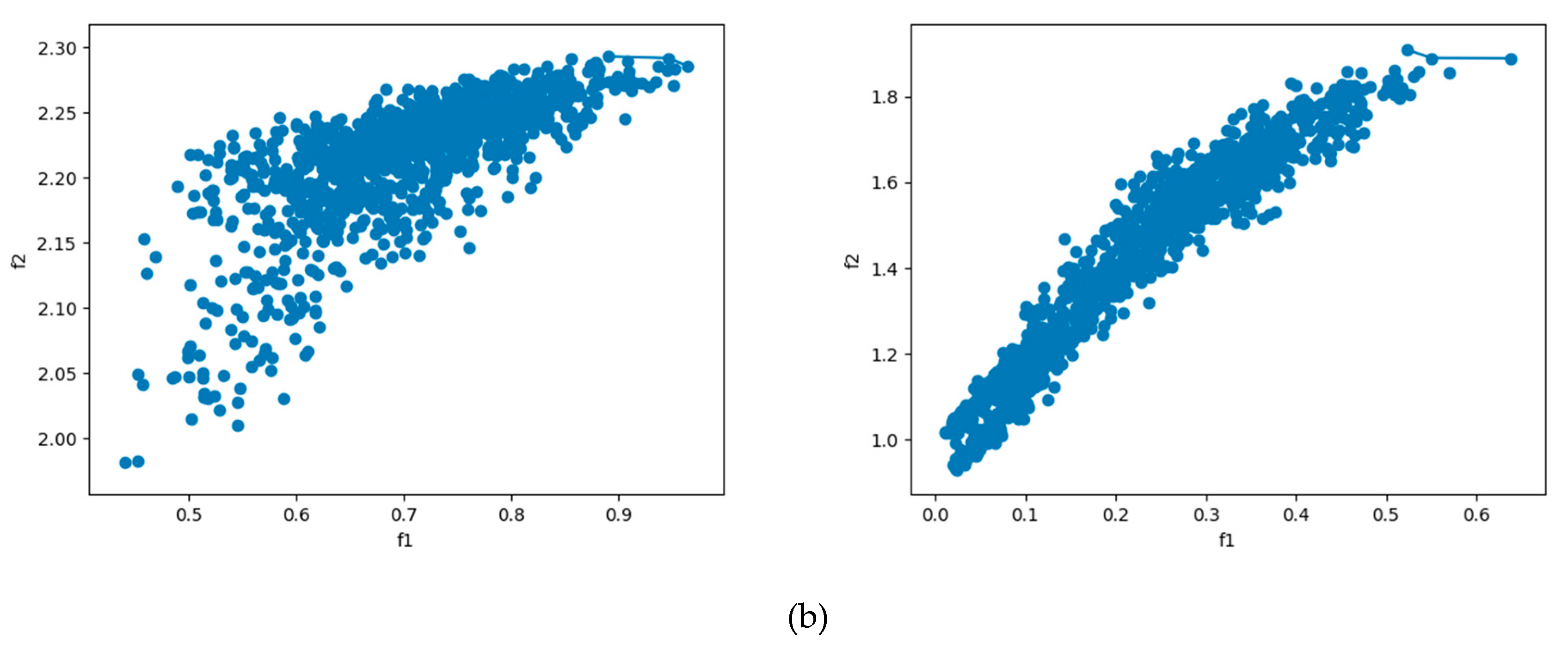
Many samples in Figure 3 are considered undesirable choices due to having low values of entropy and distance which should be dominated by other points. The samples of the pareto-set $P$ should dominate all other samples in the target domain. Thus, the samples in this set are said to be non-dominated and forms the so-called Pareto front of optimal solutions.

Figure 3. Pareto-front samples potentially indicating the presence of the unknown class.

The following Algorithm 1 provides the main steps for training the open-set DA with its nominal parameters:

Algorithm 1: Open-Set DA

Input: Source domain: $D_s={\left\{\left(X_i^{\left(s\right)},y_i^{\left(s\right)}\right)\right\}}_{i=1}^{n_s}$, and target domain: $D_t={\left\{X_j^{\left(t\right)}\right\}}_{j=1}^{n_t}$

Output: Target labels

1: Network parameters: Number of iterations $num\_iter=100$ Mini-batch size: b = 100 Adam optimizer: learning rate: 0.0001, exponential decay rate for the first and second moments ${\beta }_1=0.9$, ${\beta }_2=0.999$ and epsilon=$1e^{-8}$

2: Get feature representations from EfficientNet-B3: $h_i^{\left(s\right)}=Net\left(X^{\left(s\right)}\right)$ and $h_i^{\left(t\right)}=Net\left(X^{\left(t\right)}\right)$

3: Train the extra network on the source domain only by optimizing the loss $L_s\left(y^{\left(s_k\right)},{\widehat{y}}^{\left(s_k\right)}\right)$ for $num\_iter$

4: Classify the target domain and get $r$ samples forming the pareto set $P$ and assign them to class K+1

5: for $epoch=1:num\_iter$

5.1: Shuffle the labeled samples and organize them into $r_b=\frac{n_s+r}{b}$ groups each of size $b$

5.2: for $k=1:r_b$ Pick minibatch $k$ from these labeled samples referred as $h_k^{\left(s\right)}$ Pick randomly another minibatch of size $b$ from the target domain $h_k^{\left(t\right)}$ Update the parameters of the network by optimizing the loss in (1)

5.3: Feed the target domain samples to the network and form a new pareto set $P$

6: Classify the target domain data.

4. Experimental Results

4.1. Dataset Description

To test the performance of the proposed architecture, we used two benchmark datasets. The first dataset consists of very high resolution (VHR) images customized from three well-known remote sensing datasets, which is the Merced dataset [1] consisting of 21 category classes each with 100 images. This dataset contains images with size of 256 × 256 pixels and with 0.3-m resolution. The AID dataset contains a large number of images more than 10,000 images of size 600 × 600 pixels with a pixel resolution varying from 8 m to about 0.5 m per pixel [49]. The images are classified to different 30 classes. The NWPU dataset contains images of size of 256 × 256 pixels with spatial resolutions varying from resolution 30 to 0.2 m per pixel [50]. These images correspond to 45 category classes with 700 images for each. From these three heterogonous datasets, we build cross-domain datasets, by extracting 12 common classes (see Figure 4), where each class contains 100 images.

Figure 4. Example of samples from cross-scene dataset 1 composed of very high resolution (VHR) images.

The second dataset consists of extremely high resolution (EHR) images collected by two different Aerial Vehicle platforms. The Vaihingen dataset was captured using a Leica ALS50 system at an altitude of 500 m over Vaihingen city in Germany. Every image in this dataset is represented by three channels: near infrared (NIR), red (R), and green (G) channels. The Trento dataset contains unmanned aerial vehicles (UAV) images acquired over Trento city in Italy. These images were captured using a Canon EOS 550D camera with 2 cm resolution. Both datasets contain seven classes as shown in Figure 5 with 120 images per class.

Figure 5. Example of samples from cross-scene dataset 2 composed of extremely high resolution (EHR) images.

4.2. Experiment Setup

For training the proposed architecture, we used the Adam optimization method with a fixed learning rate of 0.001. We fixed the mini-batch size to 100 samples and we set the regularization parameter of the reconstruction error and entropy terms to 1 and 0.1, respectively.

We evaluated our approach using three proposed ranking criteria for detecting the samples of the unknown class including entropy, cosine distance, and the combination of both measures using pareto-based ranking.

We present the results in terms of (1) closed set (CS) accuracy related to the shared classes between the source and target domains, which is the number of correctly classified samples divided by the total number of tested samples of the shared classes only; (2) the open set accuracy (OS) including known and unknown classes; (3) the accuracy of the unknown class itself termed as (Unk); which is the number of correctly classified unknown samples divided by the total number of tested samples of the unknown class only, and (4) the F-measure, which is the harmonic mean of Precision and Recall:

$$F=2\times \frac{Precision\times Recall}{Precision+Recall}$$

(7)

where Recall is calculated as

$$Recall=\frac{TP}{TP+FN}$$

(8)

and Precision is calculated as

$$\mathrm{Precision}=\frac{\mathrm{TP}}{\mathrm{TP}+\mathrm{FP}}$$

(9)

where TP, FN, and FP are for true positive, false negative, and false positive, respectively. F-measure gives a value between 0 and 1. High F-measure values result in better performance for the image classification system.

For the openness measure, which is the percentage of classes that appear in the target domain and are not known in the source domain, we define it as

$$openness=1-\frac{C_S}{C_s+C_u}$$

(10)

where $C_S$ is the number of classes in the source domain shared with the target domain and $C_u$ is the number of unknown classes in the target domain. Thus, when removing three classes from the source domain this leads to nine classes in the source ($C_s$ = 9). The number of unknown classes $C_u$ is 3, which leads to an openness of $1-\frac{9}{9+3}$ = 0.25. Increasing the value of the openness leads to increasing the number of unknown classes in the target domain that are not shared by the source domain. Setting the openness to 0 is similar to the closed set architecture where all the classes are shared between source and target domains with no unknown classes in the target domain.

4.3. Results

As we are dealing with open set domain adaptation, we propose in this first set of experiments to remove three classes from each source dataset corresponding to an openness of 25%. This means that the source dataset contains nine classes while the target dataset contains 12 classes (three are unknown). Figure 6 shows the selection of the pareto-samples from the target set for the scenario AID$\to$Merced and AID$\to$NWPU during the adaptation process for the first and last iterations. Here we recall that the number of selected samples is automatically determined by the ranking process.

Figure 6. Pareto set selection from the target domain: (a) Merced$\to$AID, and (b) AID-NWPU.

As can be seen from Table 1, Table 2 and Table 3, the proposed approach exhibits promising results in leveraging the shift between the source and target distributions and detecting the presence of samples belonging to the unknown class. Table 1 shows the results when the Merced dataset is the target and the AID and NWPU are the sources, respectively. The results show that applying the domain adaptation always increases the accuracy for all scenarios, for example in the $\mathrm{AID}\to$Merced, the closed set accuracy (CS) 79.11% is lower than the results when applying the domain adaptation in all the three approaches, distance 97.77%, entropy 94.55%, and the Pareto approach 96.66%. The open set accuracy (OS) also achieves better results when the domain adaptation is applied with a minimum of 28.88% increase in the accuracy.

Table 1. Classification results obtained for the scenarios: AID$\to$ Merced and NWPU$\to$ Merced for an openness = 25%.

Target: Merced
	Source: AID				Source: NWPU
	CS	OS	Unk	F	CS	OS	Unk	F
No adapt.	79.11	59.33	0	51.81	80.33	60.25	0	53.57
Distance	97.77	90.75	69.66	88.31	97.55	73.16	0	76.25
Entropy	94.55	88.83	71.66	86.88	97.66	77.41	16.66	80.81
Pareto	96.66	88.21	62.83	86.78	97.77	85.08	47	84.48

Table 2. Classification results obtained for the scenarios: Merced$\to$ AID and NWPU$\to \mathrm{AID}$ for an openness = 25%.

Target: AID
	Source: Merced				Source: NWPU
	CS	OS	Unk	F	CS	OS	Unk	F
No adapt.	71.55	53.66	0	46.76	89.77	67.33	0	63.9
distance	87.44	83.25	70.66	74.89	98.66	83.91	39.66	82.44
Entropy	78.77	80.58	86	73.58	92.33	81.08	47.33	78.81
Pareto	93.44	88.33	73	85.22	94.66	87.33	67.33	85.07

Table 3. Classification results obtained for the scenarios: Merced$\to$ NWPU and AID$\to \mathrm{NWPU}$ for an openness = 25%.

Target: NWPU
	Source: Merced				Source: AID
	CS	OS	Unk	F	CS	OS	Unk	F
No adapt.	70.08	53.16	0	45.52	85	63.75	0	56.91
distance	69.88	61.75	37.33	55.03	89.44	74.25	28.66	68.14
Entropy	62.55	63.33	65.66	54.78	85.79	79.41	60.66	72.83
Pareto	72.77	67.75	52.66	57.6	82.77	79.16	68.33	72.22

The unknown accuracy is always 0 for all the scenarios without domain adaptation due to the negative transfer problem. The F-measure value for the $\mathrm{AID}\to$Merced scenario shows a degrade when no domain adaptation is applied with a minimum percentage of 34.97% from all other approaches. For the first scenario $\mathrm{AID}\to$Merced, the highest closed set accuracy (CS) 97.77% is achieved by the distance approach, which also gives the better open set accuracy (OS) 90.75% and F-measure value 88.31%. For the same scenario, the entropy approach results the highest unknown accuracy (Unk) 71.66%. Among the proposed selection criteria, the Pareto-based ranking achieves highest accuracies for all four metrics CS, OS, the unknown class, and the F-measure compared to other approaches in the scenario $\mathrm{NWPU}\to$Merced. The accuracy of all classes including the unknown class (OS) for this scenario is 85.08%.

Table 2 shows two scenarios where the AID dataset is the target and the Merced and NWPU are the sources, respectively. The Pareto approach gives an 88.33%, 93.44%, and 85.22% for the OS, CS, and the F-measure value, respectively, in the Merced$\to$AID scenario. For the same scenario, the highest unknown accuracy (Unk) 86% is achieved by the entropy approach. The Pareto approach achieves highest accuracies in the $\mathrm{NWPU}\to$AID scenario for the OS, Unk, and the F-measure, while the best CS accuracy is resulted from the distance method. Table 3 shows the results of the two scenarios Merced$\to \mathrm{NWPU}$ and AID$\to \mathrm{NWPU}$. The Pareto method can achieve higher results for the CS and OS 72.77% and 67.75%, respectively, for the Merced$\to \mathrm{NWPU}$ scenario, while the best unknown accuracy 65.66% is achieved by the entropy method. The AID$\to \mathrm{NWPU}$ scenario shows different results with different values of the metrics for the methods. The Pareto approach results the best unknown accuracy 68.33%, while the highest CS 89.44% is achieved by the distance approach. For the same scenario, the entropy method gives the better results for the OS and F-measure, with the values 79.41% and 72.83%, respectively. Compared to the base non-adaptation method, the Pareto approach achieves better results in all for metrics for both scenarios.

The Pareto method shows better results in most of the scenarios. Table 4 gives the results of the average accuracy (AA) for all six scenarios in Table 1, Table 2 and Table 3. The highest average accuracy for the OS is 82.64% given by the Pareto method, while for the CS is 90.12% given by the distance method which is near the 89.68% accuracy resulted by the Pareto method. The Pareto approach achieves 61.86% in the average score of unknown class. This is 3.87% higher than other methods. The Pareto approach also achieves the highest F-measure value among all other methods with an accuracy of 78.56%. The average results in Table 4 shows the effectiveness of the proposed method compared to the non-adaptation method, where the values of all four metrics in the non-adaptation method are increased by at least 10.37% in the proposed Pareto method.

Table 4. Average performances obtained for the VHR dataset.

	CS	OS	Unk	F
No adapt.	79.31	59.58	0	53.08
Distance	90.12	77.85	40.99	74.18
Entropy	85.28	78.44	57.99	74.62
Pareto	89.68	82.64	61.86	78.56

For the EHR dataset, we tested two datasets, Vaihingen and Trento. Table 5 and Table 6 show the results of the scenarios Trento$\to$Vaihingen and Vaihingen$\to$Trento, respectively. For the first scenario, the highest open set accuracy (OS) is 82.02% achieved by the Pareto approach, which also results in the highest closed set accuracy (CS) and F-measure values of 98.66% and 82.22%, respectively. The highest unknown accuracy (Unk) 51.66% is achieved by the distance approach for this scenario. The proposed Pareto method achieves better results in all four metrics compared to the base non-adaptation method. The Pareto approach achieves the highest results in all four metrics in the second scenario as shown in Table 6. The average accuracy (AA) for the two scenarios in Table 7 show that the Pareto approach achieves the best accuracies among all other approaches with an average OS accuracy 80.27%. The same method also results in the better percentage in all other three metrics used for evaluation. The average results for the two scenarios show that the proposed approach achieves a 40.52% higher open set accuracy (OS) compared to the approach where no domain adaptation is applied.

Table 5. Classification results obtained for the scenario Trento$\to$ Vaihingen.

	CS	OS	Unk	F
No adapt.	55.16	39.4	0	29.17
Distance	65.5	61.54	51.66	54.96
Entropy	97.5	71.19	5.41	72.16
Pareto	98.66	82.02	40.41	82.22

Table 6. Classification results obtained for the scenario Vaihingen$\to$ Trento.

	CS	OS	Unk	F
No adapt.	56.16	40.11	0	33.89
Distance	77.83	60	15.41	52.29
Entropy	68.83	67.38	63.75	65.29
Pareto	81.33	78.52	71.66	67.65

Table 7. Average performances obtained for the EHR dataset.

	CS	OS	Unk	F
No adapt.	55.66	39.75	0	31.53
Distance	71.66	60.77	33.53	53.62
Entropy	83.16	69.28	34.58	68.72
Pareto	89.99	80.27	56.04	74.93

5. Discussion

5.1. Effect of the Openness

In this section, we compare the robustness of the proposed Pareto approach over several openness values. The performance of the method was measured with different numbers of classes between the source and domain. As the value of openness increased, the number of unknown samples also increased which was more difficult for the classifier, compared to classifying only shared classes in the closed set classification. Table 8 shows the results obtained using different openness values for the VHR dataset. In the first scenario, we removed three classes from each source dataset corresponding to an openness of 25%. This means that the source dataset contained nine classes while the target dataset contained 12 classes (three were unknown). The highest OS accuracy was 88.33% achieved by the Merced$\to \mathrm{AID}$ scenario, while the lowest accuracy 67.75% achieved by the Merced$\to \mathrm{NWPU}$ scenario, which was 14.59% higher than the non-adaptation approach for the same scenario. The second scenario we removed four classes from the source dataset, which led to eight classes in the source dataset and 12 classes in the target dataset (four were unknown). In this scenario, the value of the accuracy degraded, resulting in 80.58% as the highest from the Merced$\to \mathrm{AID}$scenario and 69.91% as the lowest accuracy from the AID$\to \mathrm{NWPU}$ scenario. The third and fourth scenario, we removed five and six classes, respectively. The results showed that although the accuracy decreased in both scenarios, the results were still better than the non-adaptation approach. When computing the average accuracy for all six scenarios, the Pareto method achieved higher accuracy than the approach with no adaptation in all values of openness, even with an openness of 50% the Pareto method achieved an average of 63.80% accuracy with a 24.65% increase than the non-adaptation method for the same openness.

Table 8. Sensitivity analysis with respect to the openness for the VHR dataset. Results are expressed in terms of open set accuracy (OS) (%) and average accuracy (AA) (%).

Datasets	Openness (Number of Classes Removed)
	25% (3)		33.3% (4)		41.6% (5)		50% (6)
	No Adapt.	Pareto	No Adapt.	Pareto	No Adapt.	Pareto	No Adapt.	Pareto
AID$\to$Merced	59.33	88.21	50.83	79.91	47.08	61.75	38.16	61.91
$NWPU\to$Merced	60.25	85.08	50.25	79.75	44.41	78.58	39.25	66.83
Merced$\to$AID	53.66	88.33	47.75	80.58	44.5	77.58	33.0	55.33
NWPU$\to$AID	67.33	87.33	56.16	76.58	46.33	73.91	44.75	76.08
Merced$\to$NWPU	53.16	67.75	49.25	71.41	46.41	71.58	36.16	50.16
AID$\to$NWPU	63.75	79.16	55.75	69.91	46.5	69.75	43.58	72.5
AA (%)	59.58	82.64	51.66	76.35	45.87	72.19	39.15	63.80

The results of the EHR dataset, shown in Table 9 were achieved using different openness values. In the first scenario, we removed three classes from the source domain while the target domain contained seven classes leading to an openness of 42.85%. The scenario Trento$\to$Vaihingen resulted in 82.02% accuracy higher than the Vaihingen$\to$Trento which resulted in 78.52% for the openness of 42.85%. For this scenario, the Pareto approach was 40.52% higher in accuracy than the non-adaptation method which resulted in an average 39.75% accuracy for the 42.85% openness. For the second scenario we removed four classes from the source dataset. The accuracy degraded in this scenario to the values of 60.11% and 48.33% for the two scenarios, respectively. The third scenario, we removed five classes from the source dataset, resulting in an openness of 71.14%. The results of the accuracy decreased to 51.66% achieved by the Trento$\to$Vaihingen scenario. As a conclusion, we found that the proposed approach outperforms the accuracy of the non-adaptation method for different values of openness with at least 20.18%.

Table 9. Sensitivity analysis with respect to the openness for the EHR dataset. Results are expressed in terms of OS (%) and AA (%).

Datasets	Openness (Number of Classes Removed)
	42.85% (3)		57.14% (4)		71.42% (5)
	No Adapt.	Pareto	No Adapt.	Pareto	No Adapt.	Pareto
Trento $\to$Vaihingen	39.4	82.02	36.19	60.11	20.71	51.66
Vaihingen $\to$Trento	40.11	78.52	31.90	48.33	20.35	31.90
AA (%)	39.75	80.27	34.04	54.22	20.53	41.78

5.2. Effect of the Reconstruction Loss

Table 10 shows the results of the proposed method with setting the regularization parameter $\mathsf{\lambda }$ to different values in the range [0,1] for the VHR dataset. We made three scenarios with regularization parameter values of 0, 0.5, and 1. For the first scenario, the $\lambda$ was set to 0, which corresponds to the removal of the decoder part. The average accuracy dropped to 78.94%, which indicated the importance of the decoder part in the proposed method. As we can see from Table 10, setting the regularization parameter to 1 resulted in the best accuracy percentage for all scenarios except the NWPU$\to \mathrm{AID}$ which gave the highest accuracy 89.5%, when the regularization parameter was set to 0.5. The average accuracy (AA) results in Table 10 suggested that setting the regularization parameter to 1 gives better accuracy results.

Table 10. Sensitivity analysis with respect to the regularization parameter for the VHR dataset. Results are expressed in terms of OS (%) and AA (%).

Datasets	$\mathbf{Regularization}\mathbf{Parameter}\mathit{\lambda }$
	0	0.5	1
AID$\to$Merced	83.91	84.08	88.21
$\mathrm{NWPU}\to$Merced	83.25	84.16	85.08
Merced$\to$AID	79.25	80.36	88.33
NWPU$\to$AID	84.58	89.5	87.33
Merced$\to$NWPU	66.5	66.9	67.75
AID$\to$NWPU	76.16	69.75	79.16
AA (%)	78.94	79.12	82.64

The results in Table 11 show the effect of setting the regularization parameter$\mathsf{\lambda }$ to different values in the range [0,1] for the EHR dataset. We made three scenarios with regularization parameter values of 0, 0.5, and 1. The first scenario, we removed the decoder part by setting the regularization parameter $\mathsf{\lambda }$ to 0. The second and third scenario, the regularization parameter was set to 0.5 and 1, respectively. For the Trento$\to$Vaihingen scenario, removing the decoder resulted in an accuracy of 66.54%, which was a noticeable decrease from the highest accuracy 82.02% achieved when the regularization parameter was set to 1. The second scenario Vaihingen$\to$Trento also resulted in the better accuracy with the regularization parameter 1, while setting the regularization to 0.5 resulted in the worst accuracy of 51.30%. From the results shown in Table 11, setting the regularization parameter to 1 gave better accuracy results.

Table 11. Sensitivity analysis with respect to the regularization parameter for the EHR dataset. Results are expressed in terms of OS (%) and AA (%).

Datasets	$\mathbf{Regularization}\mathbf{Parameter}\mathit{\lambda }$
	0	0.5	1
Trento$\to$Vaihingen	66.54	76.90	82.02
Vaihingen$\to$Trento	59.88	51.30	78.52
AA (%)	63.21	64.1	80.27

6. Conclusions

In this paper, we addressed the problem of open-set domain adaptation in remote sensing imagery. Different to the widely known closed set domain adaptation, open set domain adaptation shares a subset of classes between the source and target domains, whereas some of the target domain samples are unknown to the source domain. Our proposed method aims to leverage the domain discrepancy between source and target domains using adversarial learning, while detecting the samples of the unknown class using a pareto-based raking scheme, which relies on the two metrics based on distance and entropy. Experiment results obtained on several remote sensing datasets showed promising performance of our model, the proposed method resulted an 82.64% openset accuracy for the VHR dataset, outperforming the method with no-adaptation by 23.06%. In the EHR dataset, the pareto approach resulted an 80.27% accuracy for the openset accuracy. For future developments, we plan to investigate other criteria for identifying the unknown samples to improve further the performance of the model. In addition, we plan to extend this method to more general domain adaptation problems such as the universal domain adaptation.

References

- Yang, Y.; Newsam, S. Bag-of-visual-words and spatial extensions for land-use classification. In Proceedings of the 18th SIGSPATIAL International Conference on Advances in Geographic Information Systems—GIS ’10; ACM Press: San Jose, CA, USA, 2010; p. 270. [Google Scholar] [CrossRef]
- Mekhalfi, M.L.; Melgani, F.; Bazi, Y.; Alajlan, N. Land-Use Classification with Compressive Sensing Multifeature Fusion. IEEE Geosci. Remote Sens. Lett. 2015, 12, 2155–2159. [Google Scholar] [CrossRef]
- Cheriyadat, A.M. Unsupervised Feature Learning for Aerial Scene Classification. IEEE Trans. Geosci. Remote Sens. 2014, 52, 439–451. [Google Scholar] [CrossRef]
- Othman, E.; Bazi, Y.; Alajlan, N.; Alhichri, H.; Melgani, F. Using convolutional features and a sparse autoencoder for land-use scene classification. Int. J. Remote Sens. 2016, 37, 2149–2167. [Google Scholar] [CrossRef]
- Huang, L.; Chen, C.; Li, W.; Du, Q. Remote Sensing Image Scene Classification Using Multi-Scale Completed Local Binary Patterns and Fisher Vectors. Remote Sens. 2016, 8, 483. [Google Scholar] [CrossRef]
- Lazebnik, S.; Schmid, C.; Ponce, J. Beyond Bags of Features: Spatial Pyramid Matching for Recognizing Natural Scene Categories. In Proceedings of the 2006 IEEE Computer Society Conference on Computer Vision and Pattern Recognition—Volume 2 (CVPR’06), IEEE, New York, NY, USA, 17–22 June 2006; Volume 2, pp. 2169–2178. [Google Scholar] [CrossRef]
- Nogueira, K.; Miranda, W.O.; Dos Santos, J.A. Improving Spatial Feature Representation from Aerial Scenes by Using Convolutional Networks. In Proceedings of the 2015 28th SIBGRAPI Conference on Graphics, Patterns and Images, Salvador, Brazil, 26–29 August 2015; pp. 289–296. [Google Scholar] [CrossRef]
- Marmanis, D.; Datcu, M.; Esch, T.; Stilla, U. Deep Learning Earth Observation Classification Using ImageNet Pretrained Networks. IEEE Geosci. Remote Sens. Lett. 2016, 13, 105–109. [Google Scholar] [CrossRef]
- Maggiori, E.; Tarabalka, Y.; Charpiat, G.; Alliez, P. Convolutional Neural Networks for Large-Scale Remote-Sensing Image Classification. IEEE Tran. Geosci. Remote Sens. 2017, 55, 645–657. [Google Scholar] [CrossRef]
- Zeng, D.; Chen, S.; Chen, B.; Li, S. Improving Remote Sensing Scene Classification by Integrating Global-Context and Local-Object Features. Remote Sens. 2018, 10, 734. [Google Scholar] [CrossRef]
- Zhu, Q.; Zhong, Y.; Liu, Y.; Zhang, L.; Li, D. A Deep-Local-Global Feature Fusion Framework for High Spatial Resolution Imagery Scene Classification. Remote Sens. 2018, 10, 568. [Google Scholar] [CrossRef]
- Liu, B.-D.; Xie, W.-Y.; Meng, J.; Li, Y.; Wang, Y. Hybrid Collaborative Representation for Remote-Sensing Image Scene Classification. Remote Sens. 2018, 10, 1934. [Google Scholar] [CrossRef]
- Lakhal, M.I.; Çevikalp, H.; Escalera, S.; Ofli, F. Recurrent neural networks for remote sensing image classification. IET Comput. Vis. 2018, 12, 1040–1045. [Google Scholar] [CrossRef]
- Wang, Q.; Liu, S.; Chanussot, J.; Li, X. Scene Classification with Recurrent Attention of VHR Remote Sensing Images. IEEE Trans. Geosci. Remote Sens. 2019, 57, 1155–1167. [Google Scholar] [CrossRef]
- Xu, S.; Mu, X.; Chai, D.; Zhang, X. Remote sensing image scene classification based on generative adversarial networks. Remote Sens. Lett. 2018, 9, 617–626. [Google Scholar] [CrossRef]
- Zhang, L.; Zhang, L.; Du, B. Deep Learning for Remote Sensing Data: A Technical Tutorial on the State of the Art. IEEE Geosci. Remote Sens. Mag. 2016, 4, 22–40. [Google Scholar] [CrossRef]
- Ye, M.; Qian, Y.; Zhou, J.; Tang, Y.Y. Dictionary Learning-Based Feature-Level Domain Adaptation for Cross-Scene Hyperspectral Image Classification. IEEE Trans. Geosci. Remote Sens. 2017, 55, 1544–1562. [Google Scholar] [CrossRef]
- Othman, E.; Bazi, Y.; Melgani, F.; Alhichri, H.; Alajlan, N.; Zuair, M. Domain Adaptation Network for Cross-Scene Classification. IEEE Trans. Geosci. Remote Sens. 2017, 55, 4441–4456. [Google Scholar] [CrossRef]
- Ammour, N.; Bashmal, L.; Bazi, Y.; Rahhal, M.M.A.; Zuair, M. Asymmetric Adaptation of Deep Features for Cross-Domain Classification in Remote Sensing Imagery. IEEE Geosci. Remote Sens Lett. 2018, 15, 597–601. [Google Scholar] [CrossRef]
- Wang, Z.; Du, B.; Shi, Q.; Tu, W. Domain Adaptation with Discriminative Distribution and Manifold Embedding for Hyperspectral Image Classification. IEEE Geosci. Remote Sens Lett. 2019, 1155-1159. [Google Scholar] [CrossRef]
- Bashmal, L.; Bazi, Y.; AlHichri, H.; AlRahhal, M.; Ammour, N.; Alajlan, N. Siamese-GAN: Learning Invariant Representations for Aerial Vehicle Image Categorization. Remote Sens. 2018, 10, 351. [Google Scholar] [CrossRef]
- Busto, P.P.; Gall, J. Open Set Domain Adaptation. In Proceedings of the 2017 IEEE International Conference on Computer Vision (ICCV) IEEE, Venice, Italy, 22–29 October 2017; pp. 754–763. [Google Scholar] [CrossRef]
- Zelnio, E.; Pavy, A. Open set SAR target classification. In Proceedings of the Algorithms for Synthetic Aperture Radar Imagery XXVI; International Society for Optics and Photonics: Bellingham, WA, USA, 2019; Volume 10987, p. 109870J. [Google Scholar] [CrossRef]
- Wang, Y.; Chen, W.; Song, J.; Li, Y.; Yang, X. Open Set Radar HRRP Recognition Based on Random Forest and Extreme Value Theory. In Proceedings of the 2018 International Conference on Radar (RADAR), IEEE, Brisbane, QLD, Australia, 27–30 August 2018; pp. 1–4. [Google Scholar] [CrossRef]
- Scheirer, W.; Rocha, A.; Sapkota, A.; Boult, T. Toward Open Set Recognition. IEEE Trans. Pattern Anal. Mach. Intell. 2013, 35, 1757–1772. [Google Scholar] [CrossRef]
- Jain, L.P.; Scheirer, W.J.; Boult, T.E. Multi-class Open Set Recognition Using Probability of Inclusion. In Computer Vision—ECCV 2014; Fleet, D., Pajdla, T., Schiele, B., Tuytelaars, T., Eds.; Springer International Publishing: Cham, Switzerland, 2014; Volume 8691, pp. 393–409. ISBN 978-3-319-10577-2. [Google Scholar] [CrossRef]
- Scherreik, M.D.; Rigling, B.D. Open set recognition for automatic target classification with rejection. IEEE Trans. Aerosp. Electron. Syst. 2016, 52, 632–642. [Google Scholar] [CrossRef]
- Wright, J.; Yang, A.Y.; Ganesh, A.; Sastry, S.S.; Ma, Y. Robust Face Recognition via Sparse Representation. IEEE Trans. Pattern Anal. Mach. Intell. 2009, 31, 210–227. [Google Scholar] [CrossRef]
- Zhang, H.; Patel, V.M. Sparse Representation-Based Open Set Recognition. IEEE Trans. Pattern Anal. Mach. Intell. 2017, 39, 1690–1696. [Google Scholar] [CrossRef] [PubMed]
- Bendale, A.; Boult, T. Towards Open World Recognition. In Proceedings of the 2015 IEEE Conference on Computer Vision and Pattern Recognition (CVPR); IEEE: Boston, MA, USA, 2015; pp. 1893–1902. [Google Scholar] [CrossRef]
- Bendale, A.; Boult, T.E. Towards Open Set Deep Networks. In Proceedings of the 2016 IEEE Conference on Computer Vision and Pattern Recognition (CVPR); IEEE: Las Vegas, NV, USA, 2016; pp. 1563–1572. [Google Scholar] [CrossRef]
- Hassen, M.; Chan, P.K. Learning a Neural-network-based Representation for Open Set Recognition. In Proceedings of the 2020 SIAM International Conference on Data Mining; Society for Industrial and Applied Mathematics: Philadelphia, PA, USA, 2020; pp. 154–162. [Google Scholar]
- Shu, L.; Xu, H.; Liu, B. DOC: Deep Open Classification of Text Documents. In Proceedings of the 2017 Conference on Empirical Methods in Natural Language Processing; Association for Computational Linguistics: Copenhagen, Denmark, 2017; pp. 2911–2916. [Google Scholar] [CrossRef]
- Shu, L.; Xu, H.; Liu, B. Unseen Class Discovery in Open-world Classification. arXiv 2018, arXiv:1801.05609. Available online: https://arxiv.org/abs/1801.05609 (accessed on 26 December 2019).
- Goodfellow, I.; Pouget-Abadie, J.; Mirza, M.; Xu, B.; Warde-Farley, D.; Ozair, S.; Courville, A.; Bengio, Y. Generative Adversarial Nets. In Advances in Neural Information Processing Systems 27; Ghahramani, Z., Welling, M., Cortes, C., Lawrence, N.D., Weinberger, K.Q., Eds.; Curran Associates, Inc.: Red Hook, NY, USA, 2014; pp. 2672–2680. [Google Scholar]
- Ge, Z.; Demyanov, S.; Chen, Z.; Garnavi, R. Generative OpenMax for multi-class open set classification. In Proceedings of the British Machine Vision Conference Proceedings 2017; British Machine Vision Association and Society for Pattern Recognition: Durham, UK, 2017. [Google Scholar] [CrossRef]
- Neal, L.; Olson, M.; Fern, X.; Wong, W.-K.; Li, F. Open Set Learning with Counterfactual Images. In Computer Vision—ECCV 2018; Ferrari, V., Hebert, M., Sminchisescu, C., Weiss, Y., Eds.; Springer International Publishing: Cham, Switzerland, 2018; Volume 11210, pp. 620–635. ISBN 978-3-030-01230-4. [Google Scholar] [CrossRef]
- Yu, Y.; Qu, W.-Y.; Li, N.; Guo, Z. Open-category classification by adversarial sample generation. In Proceedings of the 26th International Joint Conference on Artificial Intelligence; AAAI Press: Melbourne, Australia, 2017; pp. 3357–3363. [Google Scholar]
- Saito, K.; Yamamoto, S.; Ushiku, Y.; Harada, T. Open Set Domain Adaptation by Backpropagation. In Computer Vision—ECCV 2018; Ferrari, V., Hebert, M., Sminchisescu, C., Weiss, Y., Eds.; Springer International Publishing: Cham, Switzerland, 2018; Volume 11209, pp. 156–171. ISBN 978-3-030-01227-4. [Google Scholar] [CrossRef]
- Cao, Z.; Long, M.; Wang, J.; Jordan, M.I. Partial Transfer Learning with Selective Adversarial Networks. In Proceedings of the 2018 IEEE/CVF Conference on Computer Vision and Pattern Recognition, Salt Lake City, UT, USA, 18–22 June 2018; pp. 2724–2732. [Google Scholar] [CrossRef]
- Zhang, J.; Ding, Z.; Li, W.; Ogunbona, P. Importance Weighted Adversarial Nets for Partial Domain Adaptation. In Proceedings of the 2018 IEEE/CVF Conference on Computer Vision and Pattern Recognition, Salt Lake City, UT, USA, 18–22 June 2018; pp. 8156–8164. [Google Scholar] [CrossRef]
- Baktashmotlagh, M.; Faraki, M.; Drummond, T.; Salzmann, M. Learning factorized representations for open-set domain adaptation. In Proceedings of the International Conference on Learning Representations (ICLR), New Orleans, LA, USA, 6–9 May 2019. [Google Scholar]
- Lian, Q.; Li, W.; Chen, L.; Duan, L. Known-class Aware Self-ensemble for Open Set Domain Adaptation. arXiv 2019, arXiv:1905.01068. Available online: https://arxiv.org/abs/1905.01068 (accessed on 26 December 2019).
- Liu, H.; Cao, Z.; Long, M.; Wang, J.; Yang, Q. Separate to Adapt: Open Set Domain Adaptation via Progressive Separation. In Proceedings of the 2019 IEEE/CVF Conference on Computer Vision and Pattern Recognition (CVPR), IEEE, Long Beach, CA, USA, 16–20 June 2019; pp. 2922–2931. [Google Scholar] [CrossRef]
- Tan, S.; Jiao, J.; Zheng, W.-S. Weakly Supervised Open-Set Domain Adaptation by Dual-Domain Collaboration. In Proceedings of the 2019 IEEE/CVF Conference on Computer Vision and Pattern Recognition (CVPR), IEEE, Long Beach, CA, USA, 16–20 June 2019; pp. 5389–5398. [Google Scholar] [CrossRef]
- Tan, M.; Le, Q. EfficientNet: Rethinking Model Scaling for Convolutional Neural Networks. In Proceedings of the International Conference on Machine Learning, Long Beach, CA, USA, 9–15 June 2019; pp. 6105–6114. [Google Scholar]
- Saito, K.; Kim, D.; Sclaroff, S.; Darrell, T.; Saenko, K. Semi-Supervised Domain Adaptation via Minimax Entropy. In Proceedings of the 2019 IEEE/CVF International Conference on Computer Vision (ICCV), IEEE, Seoul, Korea, 27 October–2 November 2019; pp. 8049–8057. [Google Scholar]
- Ganin, Y.; Lempitsky, V. Unsupervised domain adaptation by backpropagation. In Proceedings of the 32nd International Conference on Machine Learning—Volume 37; Lille, France, 7–9 July 2015; JMLR.org: Lille, France, 2015; pp. 1180–1189. [Google Scholar]
- Xia, G.-S.; Hu, J.; Hu, F.; Shi, B.; Bai, X.; Zhong, Y.; Zhang, L. AID: A Benchmark Dataset for Performance Evaluation of Aerial Scene Classification. IEEE Trans. Geosci. Remote Sens. 2017, 55, 3965–3981. [Google Scholar] [CrossRef]
- Cheng, G.; Han, J.; Lu, X. Remote Sensing Image Scene Classification: Benchmark and State of the Art. Proc. IEEE 2017, 105, 1865–1883. [Google Scholar] [CrossRef]
© 2020 by the authors. Licensee MDPI, Basel, Switzerland. This article is an open access article distributed under the terms and conditions of the Creative Commons Attribution (CC BY) license (http://creativecommons.org/licenses/by/4.0/).