Article

CO2 Concentration, A Critical Factor Influencing the Relationship between Solar-induced Chlorophyll Fluorescence and Gross Primary Productivity

1
School of Remote Sensing and Information Engineering, Wuhan University, Wuhan 430079, China
2
State Key Laboratory of Information Engineering in Surveying, Mapping and Remote Sensing, Wuhan University, Wuhan 430079, China
3
School of Environmental Science and Tourism, Nanyang Normal University, Nanyang 473061, China
*
Author to whom correspondence should be addressed.
Remote Sens. 2020, 12(9), 1377; https://doi.org/10.3390/rs12091377
Submission received: 13 February 2020 / Revised: 21 April 2020 / Accepted: 24 April 2020 / Published: 27 April 2020

Abstract

:
The uncertainty of carbon fluxes of the terrestrial ecosystem is the highest among all flux components, calling for more accurate and efficient means to monitor land sinks. Gross primary productivity (GPP) is a key index to estimate the terrestrial ecosystem carbon flux, which describes the total amount of organic carbon fixed by green plants through photosynthesis. In recent years, the solar-induced chlorophyll fluorescence (SIF), which is a probe for vegetation photosynthesis and can quickly reflect the state of vegetation growth, emerges as a novel and promising proxy to estimate GPP. The launch of Orbiting Carbon Observatory 2 (OCO-2) further makes it possible to estimate GPP at a finer spatial resolution compared with Greenhouse Gases Observing Satellite (GOSAT), Global Ozone Monitoring Experiment-2 (GOME-2) and SCanning Imaging Absorption spectroMeter for Atmospheric CHartographY (SCIAMACHY). However, whether the relationship between GPP and SIF is linear or non-linear has always been controversial. In this research, we proposed a new model to estimate GPP using SIF and the atmospheric CO2 concentration from OCO-2 as critical driven factors simultaneously (SIF-CO2-GPP model). Evidences from all sites show that the introduction of the atmospheric CO2 concentration improves accuracies of estimated GPP. Compared with the SIF-CO2-GPP linear model, we found the SIF-GPP model overestimated GPP in summer and autumn but underestimated it in spring and winter. A series of simulation experiments based on SCOPE (Soil-Canopy Observation of Photosynthesis and Energy) was carried out to figure out the possible mechanism of improved estimates of GPP due to the introduction of atmospheric CO2 concentrations. These experiments also demonstrate that there could be a non-linear relationship between SIF and GPP at half an hour timescale. Moreover, such relationships vary with CO2 concentration. As OCO-2 is capable of providing SIF and XCO2 products with identical spatial and temporal scales, the SIF-CO2-GPP linear model would be implemented conveniently to monitor GPP using remotely sensed data. With the help of OCO-3 and its successors, the proposed SIF-CO2-GPP linear model would play a significant role in monitoring GPP accurately in large geographical extents.

Graphical Abstract

1. Introduction

The carbon flux of terrestrial ecosystems, with the greatest uncertainty, plays an important role in the carbon cycle [1]. Terrestrial carbon fluxes are fundamental to understand the feedback mechanism of terrestrial ecosystems to climate change [2]. However, the imbalance between carbon sources and carbon sinks results in the so-called “mystery of the missing carbon” [3,4]. Therefore, there is an urgent need to obtain accurate estimates of terrestrial carbon fluxes [5]. Gross primary productivity (GPP) is an important indicator for estimating terrestrial carbon fluxes. GPP refers to the amount of organic carbon fixed by green plants through photosynthesis per unit time; thus, it determines the initial substances and energy entering terrestrial ecosystems [6,7]. Therefore, an accurate estimation of GPP is an indispensable step to reduce the uncertainty of terrestrial carbon fluxes.
The eddy covariance (EC) technology is seen as the most accurate method to estimate GPP. The main features obtained by the EC technology include semi-hourly/hourly fluxes of CO2, heat and humidity. Ecosystem respiration (ER) is calculated by interpolating Net Ecosystem Exchange (NEE) and temperature (T) [8,9,10,11]. Then, GPP is calculated as the difference between ER and NEE. The flux-tower-derived GPP products have clear advantages in the accuracy compared with remote sensing products. However, the footprint of observations of flux towers is small, resulting in a lack of spatial representativeness. Moreover, the number of flux towers is insufficient to monitoring GPP globally, and the uneven distribution of flux towers further left huge gaps in many regions. Satellite observations can serve as a good supplement to flux towers in terms of spatial coverage despite relatively lower accuracy of GPP estimates. For example, MODIS GPP is calculated using the light use efficiency (LUE) model [12]. The LUE model is the product of three variables fPAR (the proportion of PAR absorbed by plant canopies), PAR (photosynthetically active radiation) and LUEP (light use efficiency). LUEP indicates the efficiency of the radiation absorbed by the vegetation during photosynthesis [13]. LUEP is the critical input parameter of the LUE model, which is susceptible to plant growth status and ecological environments. Therefore, the light use efficiency should vary with different environments and growth stages of vegetation theoretically. However, LUEP is generally determined as a fixed parameter in the LUE model according to specific vegetation types, resulting in large uncertainties of estimated GPP. In addition, the LUE model requires a large number of ground parameter inputs, and the uncertainty of those parameters will also propagate to estimates of GPP [14,15].
Solar-induced chlorophyll fluorescence (SIF) is a probe of vegetation photosynthesis because most changes in photosynthesis can be reflected by SIF. Hence, SIF opens a new prospect for GPP estimations [16,17]. Previous studies have demonstrated that SIF-estimated GPP is more accurate than that of LUE model mainly because SIF is a byproduct of photosynthesis. Hence, water and heat stress on photosynthesis processes can be reflected by changes in chlorophyll fluorescence immediately [12,18]. Recent studies show that the accuracy of SIF-estimated GPP is evidently higher than those estimated by other vegetation indexes, such as the normalized difference vegetation index (NDVI) and enhanced vegetation index (EVI) [12,18,19]. Some researchers used SIF to calculate Vcmax (maximum carboxylation capacity), which presented a better GPP estimation accuracy [20,21]. SIF products from the Greenhouse Gases Observing Satellite (GOSAT) [22], the Global Ozone Monitoring Experiment-2 (GOME-2) [23] and the SCanning Imaging Absorption spectroMeter for Atmospheric CHartographY (SCIAMACHY) [24] were used to establish models to estimate GPP in the past a few years. Along with the launch of the Orbiting Carbon Observatory 2 (OCO-2) in 2014, a new SIF product is now available to estimate GPP at a finer spatial resolution (1.3 × 2.25 km), comparing with previous products from GOME-2 (40 × 40 km) and GOSAT (10km diameter) [22]. The main task of OCO-2 is to map the global atmospheric CO2 concentration by recording the sunlight reflected from the Earth’s surface. The main sensor of OCO-2 consists of three high-resolution spectrometers that make coincident measurements of reflected sunlight in the 1.61 (CO2 weak absorption), 2.06 (CO2 strong absorption) and 0.76 μm (O2 A-Band) bands. The SIF product can be retrieved using IMAP-DOAS algorithm of NASA. The general principle of retrieving SIF is based on the filling of Fraunhofer solar lines. Measuring the partial depth of Fraunhofer spectral lines, which decreases with the presence of surface SIF radiation. Previous studies have shown that there is a strong linear/nonlinear relationship between SIF products of OCO-2 and GPP [25,26]. However, the SIF signal can be affected by solar and viewing zenith angles [27]. Moreover, the atmospheric CO2 concentration is another important factor affecting vegetation photosynthesis and GPP [28]. Existing studies have confirmed that the increasing atmospheric CO2 concentration promotes the rate of photosynthesis of tomato plants on the scale of individual plants [29]. On the scale of larger vegetation distribution, previous studies also demonstrated that CO2 has a significant impact on the total primary productivity of vegetation [30,31,32]. However, current studies on estimating GPP using satellite-derived SIF products ignored the possible effect of atmospheric CO2 concentrations on modeling GPP. The SIF-GPP model could be further improved by the introduction of a new parameter, namely, the atmospheric CO2 concentration. Therefore, we propose to investigate the effect of atmospheric CO2 concentrations on estimating GPP using SIF products. Because OCO-2 provides of column-averaged CO2 dry air mole fraction, abbreviated as XCO2 hereafter, and SIF simultaneously. Which will be very easy to take the atmospheric CO2 concentration into the new model of GPP.
The rest of this work is organized as follows. Section 2 introduces the study area, datasets and methods. The results are demonstrated in Section 3. Discussions are provided in Section 4. Finally, we conclude the whole study in Section 5.

2. Materials and Methods
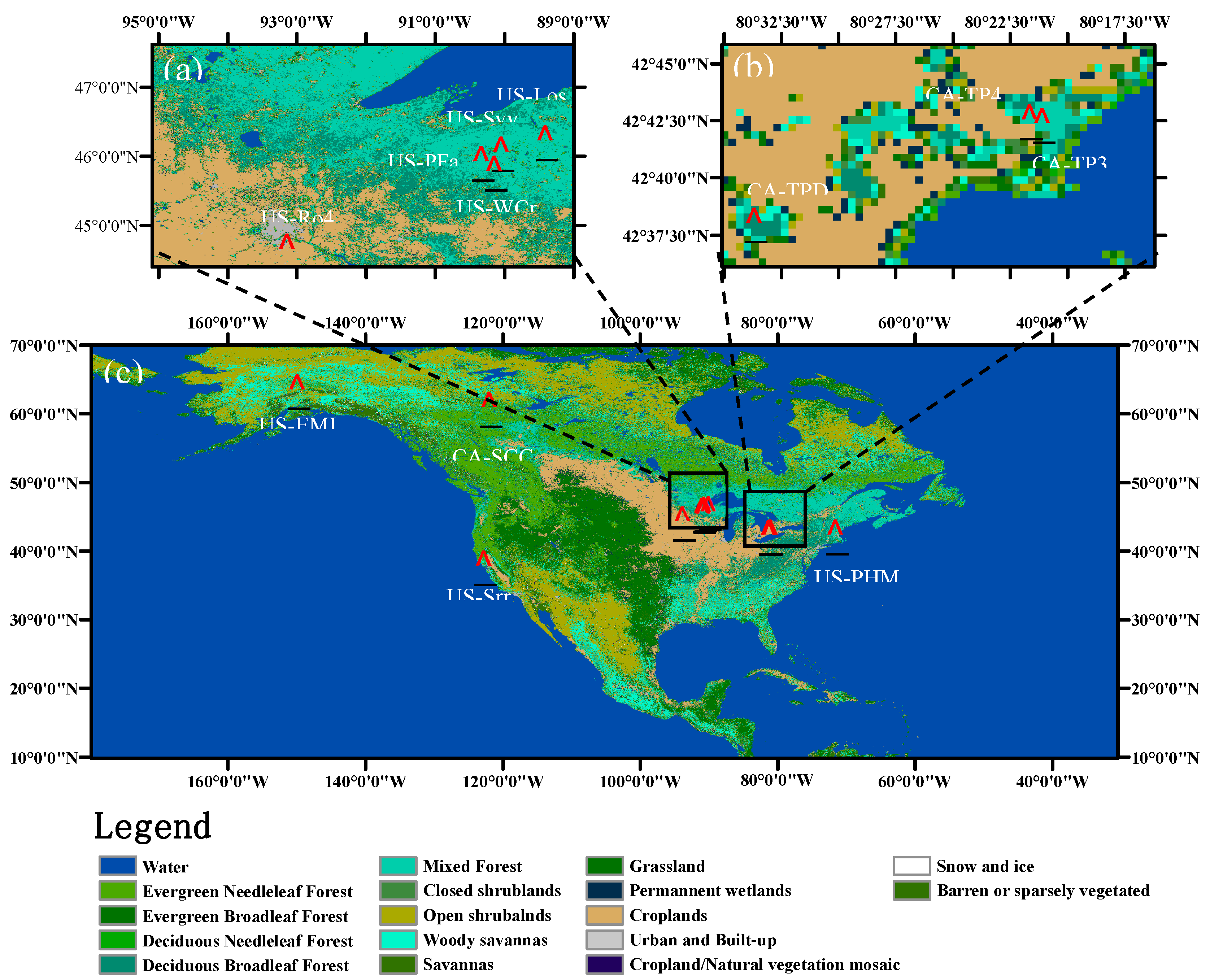
2.1. Study Area

In order to find a suitable study area, we screened all flux towers coinciding geographically with OCO-2 footprints in North America. Finally, we chose 12 EC flux sites in North America as shown in Figure 1, because both EC flux data and OCO-2 data are available, and vegetation types are homogeneous at those sites. There are 6 major biome types, namely, Evergreen Needleleaf Forests (3 sites), Mixed Forests (2 sites), Deciduous Broadleaf Forests (2 sites), Permanent Wetlands (3 sites), Grasslands (1 site) and Open shrublands (1 site). More details of selected sites are described in Table 1. Those sites are most in the mid-latitude region, ensuring that there are adequate OCO-2 data. Besides, both SIF and GPP products are available at these sites.

2.2. Data Source

In this study, the datasets used included OCO-2 products, EC Flux Tower datasets and MODIS data. We used SIF and XCO2 data from OCO-2. The data versions of SIF and XCO2 are OCO2_L2_Lite_SIF.8r and OCO2_L2_Lite_FP.8r, respectively. The SIF product was calculated using the IMAP-DOAS algorithm. The SIF product was retrieved using two Fraunhofer lines centering at 757 nm and 771 nm, respectively. There are three observation modes for OCO-2, namely, nadir, glint and target mode. In order to avoid additional errors, we only select SIF products in the same observation mode for each site. If there are SIF products with more than two observation modes for a single site, the observation mode with the largest amount of data was selected. With that criterion, we used SIF data of target mode for US-PFa and US-WCr, used those of glint mode for CA-TPD. For the rest of the sites, we used SIF data of nadir mode. Moreover, we extracted XCO2 data and their corresponding quality identification from OCO-2 datasets spanning from 2014 to 2019.
In this study, we used land cover classification 2 (University of Maryland UMD format) of MCD12Q1 from MODIS as auxiliary data to evaluate the study area. Land cover types of North America contain 17 different types. Different vegetation types are represented by different colors. (Figure 1). Due to the proximity of several selected study areas to each other, we have expanded some of the study areas to provide a clear description of the locations of these flux towers. In addition to remote sensing products, we also used GPP and surface CO2 concentrations from EC flux towers. Both of these products were downloaded from the Ameriflux website.
We did a preliminary processing of the data. XCO2 data with “xCO2_quality_flag” equal to 1 were also eliminated. For EC tower’s products, there are several missing measurements in the original products of the surface CO2 mole fraction and GPP measurements. We have applied spline interpolation to fill these missing values. For the CO2 data of the flux tower, we take the frictional wind speed 0.2 as the threshold value. Only when the frictional wind speed is greater than 0.2 can we consider the CO2 data to be valid [33].

2.3. Method

The core idea of this work is to prove that the atmospheric CO2 concentration is a critical factor determining the performances of modelling GPP using OCO-2 SIF data. Based on that, we try to propose a SIF-CO2-GPP model to better reproduce GPP. Hence, there are several procedures to be followed. Firstly, we need to determine which SIF product of OCO-2 datasets would be more appropriate as the input of the SIF-GPP model /SIF-CO2-GPP model. Secondly, we need to figure out the most suitable timescale in modeling GPP using SIF. After that, it is the most important part of this work to compare the performances of commonly used SIF-GPP model and propose the SIF-CO2-GPP model. On that basis, we need to prove there is a strong relationship between the surface CO2 concentration and XCO2 so that all inputs of the SIF-CO2-GPP model would be obtained from satellite-based means. Finally, it is also necessary to find out plausible mechanisms to explain why and how the inclusion of CO2 concentration helps promoting performances of modeling GPP using SIF.

2.3.1. The Linear Relationship of EC GPP and OCO-2 SIF at Different Bands and Timescales

Figure 2 shows the workflow of this study. First of all, we tried to evaluate the performances of SIF-GPP models in terms of the timescale. Therefore, SIF-GPP models were established using instantaneous and daily SIF data, respectively. We selected the OCO-2 product within 10 km of the EC tower for comparison with the GPP product of the EC flux tower. The SIF product of OCO-2 is the instantaneous data in two bands, 757 nm (ins757) and 771 nm (ins771). We also converted the instantaneous SIF data to daily data (SIF757 and SIF771) using the daily average correction factor from the OCO-2 L2 file. Since the average of SIF771 is 1.2 to 1.5 times smaller than SIF757, we multiplied the value of SIF771 by 1.5. For the convenience of comparison, the value of SIF771 is multiplied by 1.2–1.5. We multiplied the value of SIF771 by a factor of 1.5. The instantaneous GPP (insGPP) is calculated as the average of hourly/semi-hourly GPP data between 1:00 and 2:00 pm local time. In this study, all EC tower stations provide semi-hourly GPP except US-PFa, which provides hourly GPP data. On that basis, linear correlations between instantaneous SIF data (ins757 and ins771) and instantaneous GPP (insGPP) were established and analyzed. Moreover, we converted the hourly/semi-hourly GPP data of EC towers to daily GPP after filling some missing data using an interpolation process. Then, we have examined the linear correlation between daily SIF (SIF757 and SIF 771) and daily GPP. Furthermore, we compared performances of linear models those utilize SIF data of different bands (757 nm and 771 nm) as independent variables at both timescales to find out which SIF data is more suitable for estimating GPP. In evaluations of linear models, goodness of fit, R2, is used to describe the degree of interpretation of GPP by SIF. The correlation coefficient (R) indicates how close the two variables are. We used p to represent the significance of the model. It is generally considered that the linear analysis is significant when p value is less than 0.005.

2.3.2. SCOPE Model

Theoretically, the atmospheric CO2 concentration could be an important factor affecting photosynthesis of vegetation, and many studies have shown that CO2 has a fertilizing effect on most vegetation [28,34,35]. In this study, SCOPE model (Soil-Canopy Observation of Photosynthesis and Energy) is used to explore the mechanism of how CO2 affects GPP estimation. SCOPE model is a vertical (1-D), integrated, radiative transfer and energy balance model [36], which can be applied to the quantitative study of canopy fluorescence spectrum and net photosynthetic of the canopy. SCOPE model consists of two modules: Fluspect, which is used to simulate the radiation transmission of reflected light, transmitted light and fluorescence inside the blade, and Biochemical module, which is used to calculated the photosynthetic rate and the ratio of absorbing radiation to fluorescence in C3 and C4 plants [37].
In this study. Firstly, we used the SCOPE model to simulate GPP with a varying SIF and different settings of atmospheric CO2 concentrations. Then, we can analyze the effect of different CO2 concentrations on the linear relationship of SIF-GPP. The required input parameters of the SCOPE model include meteorological data (incoming shortwave and long-wave radiation, air temperature, humidity, wind speed and CO2 concentration), leaf area index(LAI), leaf angle distribution, leaf chlorophyll content(Cab), stomatal conductance parameter (m), maximum carboxylation capacity(Vcmo) and so on. In order to explore the effect of the CO2 concentrations on daily variation characteristics of vegetation canopy GPP and SIF, the model parameters were set as follows: (1) Biochemical parameters: Set Vcmo to 90 according to Kothavala’s work [38]. When C3 plants have enough water m(Ball-Berry stomatal conductance parameter) should be set to 9 [39]. Dark respiration (Rdparam) was set to 0, so that the net photosynthesis of canopy output is equivalent to GPP [40]. (2) The meteorological data, which spans from 8:00 am to 18:00 pm on April 14, 2015, with a time resolution of half an hour, were acquired from US-Syv flux towers. (3) Finally, the atmospheric CO2 concentration was set to 8 levels, namely, 300, 350, 375, 400, 425, 450, 475 and 500 ppm. The remaining input parameters were set as defaults of the SCOPE model.

2.3.3. Detection of CO2 Correction for SIF-GPP Model

In order to explore the impact of atmospheric CO2 concentrations on estimating GPP, we constructed a SIF-CO2-GPP linear model to estimate GPP and compared it with the frequently used SIF-GPP model. When constructing the SIF-CO2-GPP model, we used the surface CO2 mole fraction data of the EC flux towers. The SIF-CO2-GPP model utilizes the daily SIF757 as the primary variable and the CO2 mole fraction as the secondary variable to estimate GPP (Hereafter, GPPM represents the result of the SIF-CO2-GPP model while GPPS represents the result of the SIF-GPP model). We used the method of k-fold cross validation to compare the SIF-GPP model with the SIF-CO2-GPP model. In other words, the samples were divided into k portions. These k-1 portions were used for establishing the model and 1 portion was used for validation. Then we repeated k times of the above procedures so that all samples were used for the validation. For sites that have more than 10 samples, k is 10. Otherwise, k is 4. By comparing performances of the SIF-GPP model and the SIF-CO2-GPP model, we tried to find out whether the introduction of CO2 mole fraction can improve the accuracy of estimating GPP, since the ultimate goal of both models is to estimate the regional GPP by remotely sensed proxy parameters. Here we conduct additional experiments to investigate the relationship between the surface CO2 molar fraction measured by the EC flux tower and the XCO2 obtained by OCO-2. We selected four flux towers with sufficient XCO2 data to establish a linear relationship between surface CO2 molecular weight and XCO2. Since the EC flux tower and the OCO-2 footprint barely overlap, the XCO2 data for OCO-2 within 10 km of the EC flux tower were averaged and compared to the surface CO2 molar fraction measured in the EC flux tower. Finally, the gridded GPPS and GPPM were produced using OCO-2 products in surroundings of US-PFa on four representative days of different seasons. The coverage and spatial resolution are ~20 × 20 km and 1 km, respectively. Differences between areal GPPS and GPPM were demonstrated in terms of spatial and temporal scales.

3. Results

3.1. Selection of Appropriate Bands and Timescales

Figure 3 illustrates the linear relationship between instantaneous SIF of different bands and instantaneous GPP. In general, there is a strong linear relationship between SIF and GPP. For most towers, ins757 was more strongly correlated to tower-measured GPP than ins771. Therefore, the ins757 could be a better proxy to estimate instantaneous GPP than ins771. Our results are consistent with the hypothesis of a previous study [18]. A plausible reason to explain such results would be that 771 nm is farther away from the peak of SIF spectrum than 757 nm. We also speculate that the insufficient sample size would lead to an unstable and inaccurate model and that could be responsible for the exception [12].
The linear relationships between daily SIF and daily GPP at 12 sites were shown in Figure 4. Overall, R2 of linear models for daily GPP estimating are evidently higher than those for instantaneous GPP. Besides, the advantage of SIF products of 757 nm has been further strengthened over SIF products of 771 nm in terms of estimations of daily GPP. Consequently, we concluded that OCO-2 SIF products of 757 nm are better than those of 771 nm in estimating GPP, and it is better to estimate daily GPP than instantaneous GPP. In order to figure out which timescale of the SIF data is more suitable for estimating GPP, we compare the coefficient of determination R2 of ins757-GPP and daily757-GPP in Table 2. Except for CA-TP4, CA-SCC, US-EML and US-Los, R2 of -SIF757-GPP at other sites is significantly higher than that of ins757-GPP. Therefore, we can conclude that daily SIF data is more suitable for estimating GPP.

3.2. The Performance is Improved Due to the Addition of CO2

Table 3 demonstrates the fitted formulae and R2 of SIF-GPP models and SIF-CO2-GPP models. R2 of models surges after the introduction of surface CO2 concentrations, implying that the CO2 concentration plays a critical role in modeling GPP. In statistics, the coefficient of determination (R2) indicates the ability of the dependent variable to predict the dependent variable. A significant increase in R2 indicates that surface CO2 concentration is a non-negligible variable for estimating GPP. In all 12 sites, R2 was improved to varying degrees at all 12 sites (3%–41%) after the introduction of the surface CO2 concentrations. Table 3 also shows an interesting a phenomenon that the increase rate has a negative correlation with R2 of the SIF-GPP model. Table 3 also shows an interesting phenomenon, as 9 of the 12 study sites had negative CO2 coefficients in the study area. The increase of model performance due to the introduction of CO2 could be explained by the fact that the effect of CO2 correction mitigates the non-linear relationship between daily SIF and daily GPP. It is worth noting that it is by no means negative coefficients of CO2 imply a high CO2 concentration would cause a decreasing of GPP because the linear regression indicates a correlation but not causality. Details on a possible mechanism on how CO2 concentrations regulate GPP will be discussed in Section 4.1 and Section 4.2.
Figure 5 shows linear relationships between modeled GPP and measured GPP in different sites. We used the measured GPP of EC Flux towers represents truth value. Then, we used the method of leave-one-out cross validation to compare the SIF-GPP model with the SIF-CO2-GPP model. R of GPP-GPPM is higher than that of GPP-GPPS at all sites. We also calculated root-mean-square error (RMSE), which represents the deviation between the estimates of models and true values (Table 4). The RMSE of SIF-CO2-GPP models are lower than those of SIF-GPP models at 8 out of 12 sites, suggesting better performances of SIF-CO2-GPP models. In the meantime, slopes of linear relationships between GPP and GPPM are much more close to 1 than those between GPP and GPPS. All the above results indicate that the SIF-CO2-GPP model is superior to the traditional SIF-GPP model.

3.3. Relationships between XCO2 and Surface CO2 Mixing Ratio

In Table 3, we used the surface CO2 mixing ratio measured by EC flux towers as the input of the SIF-CO2-GPP models. However, the ultimate goal of the proposed model is to map distributions of GPP in large extents. Hence, it is critical to find an appropriate proxy to the surface CO2 mixing ratio. XCO2 is the main products of OCO-2. Both XCO2 and SIF products are retrieved from spectral measurements of OCO-2. Therefore, XCO2 and SIF products of OCO-2 share the same footprints with respect to both time and space dimensions. If there was a robust relationship between surface CO2 mixing ratio and XCO2, it would be a key foundation for mapping GPP globally using the proposed SIF-CO2-GPP model. Hence, additional experiments were conducted to investigate the relationship between the CO2 mixing ratio observed in the EC flux tower (hereafter referred to as tower CO2) and the XCO2 product of OCO-2. For this sake, we carried out an additional experiment to explore the relationship between surface CO2 mixing ratio of EC flux towers, abbreviated as Tower CO2 hereafter, and XCO2 products of OCO-2. Figure 6 illustrates the linear correlation between XCO2 of OCO-2 and Tower CO2. x represents XCO2 of OCO-2 while y stands for Tower CO2, and N is the number of valid samples. CA-TP4, CA-TPD and US-Syv had less than 8 samples, resulting in an unreliable relationship between XCO2 and tower CO2. Therefore, these sites were excluded from this experiment. First of all, R between XCO2 and Tower CO2 fluctuate between 0.54 and 0.87, showing there are strong linear correlation between XCO2 and Tower CO2. That feature would be very beneficial to replacing surface CO2 mixing ratio by XCO2 in the SIF-CO2-GPP model. Meanwhile, it is also illustrated that slopes of linear relationship between XCO2 and tower CO2 deviate significantly from 1. It is hence concluded that there is need for correlating XCO2 and surface CO2 mixing ratio by means of observations and atmospheric models. Another alternative solution is to directly establish the SIF-CO2-GPP model using XCO2 instead of Tower CO2 if there were adequate valid samples.

3.4. Mapping GPP using OCO-2 SIF and XCO2 Products

Finally, we have mapped the gridded GPP based on the traditional SIF-GPP model and SIF-CO2-GPP model to explore new features of the proposed model. In this experiment, we used SIF757 and XCO2 products of OCO-2 spanning from 2015 to 2016, which are around 20 km of US-PFa, to generate GPPM and GPPS products with a spatial resolution of 1km (14 April 2015, 1 June 2015, 14 September 2016, 1 November 2016). Though the data amount of SIF and XCO2 products around US-PFa is the largest in all 12 sites, there are still considerable missing data, especially for 1 November 2016, which results in blank parts in Figure 7.
Figure 7 shows gridded GPPS and GPPM on 4 representative days of different seasons around US-PFa EC flux tower. Overall, GPPS and GPPM products exhibit similar seasonality, i.e., high GPP in summer and fall and low GPP in spring and winter. In the spring, the vegetation begins to grow along with the rising temperature. Hence, GPP in spring is higher than GPP in winter. The mean GPP of summer is the highest in all seasons because the driven parameter of GPP-estimating model, SIF, reaches peak in summer along with the strong effect of photosynthesis. The date we chose for autumn belongs to early autumn in this study. The vegetation has not completely withered, resulting in a higher GDP in the fall simulation than in the spring. In winter, the photosynthesis of vegetation becomes weak because of the low temperature. The mean annual temperature of US-PFa is 4.33 °C in winter. Hence, the mean GPP drops to the lowest. We averaged all the GPP grids data estimated by SIF-CO2-GPP model and SIF-GPP model within 20 × 20 km for each day. Then, we compared the modeled GPP and measured GPP. The measured GPP of flux towers are 2.09, 7.03, 4.15 and 1.59 for four representative days (Apr 14, 2015, Jun 1, 2015, Sep 14, 2016, and Nov 1, 2016). The unit is g Cm−2d−1. The mean GPPM estimated by SIF-CO2-GPP model are 2.09, 6.90, 4.33 and 1.61. The mean GPPS estimated by SIF-GPP model are 1.84, 7.93, 4.45 and 1.43. Therefore, it is concluded that the SIF-CO2-GPP model is more suitable for estimating GPP and yields a higher precision than the SIF-GPP model.
On the whole, there are evident differences between GPPS and GPPM in spring, summer, autumn, and winter. The SIF-CO2-GPP model leans to overestimate GPP in spring and winter, but underestimate GPP in summer and autumn, comparing with the SIF-GPP model. The value of GPPM is closer to the measured GPP value of the flux tower, which indicates to some extent that the SIF-CO2-GPP model is able to estimate GPP with higher accuracy. Therefore, we can conclude that the effect of CO2 is not simply shrinking or amplifying estimated GPP. The introduction of CO2 helps reduce estimated GPP in some conditions but helps increase estimated GPP in other conditions. This is why we argue that negative coefficients of CO2, as shown in Table 3, should not be attributed to a high CO2 concentration causing a decrease in GPP or vice versa. We should notice that the level of CO2 concentration is regulated by the intensity of the photosynthesis. Consequently, it is impossible to keep the CO2 concentration at a constant level under natural conditions when the intensity of SIF is varying. To explore and explain the correction effect of the CO2 concentration on GPP, we carried out extra simulation experiments using the SCOPE model in the next section.

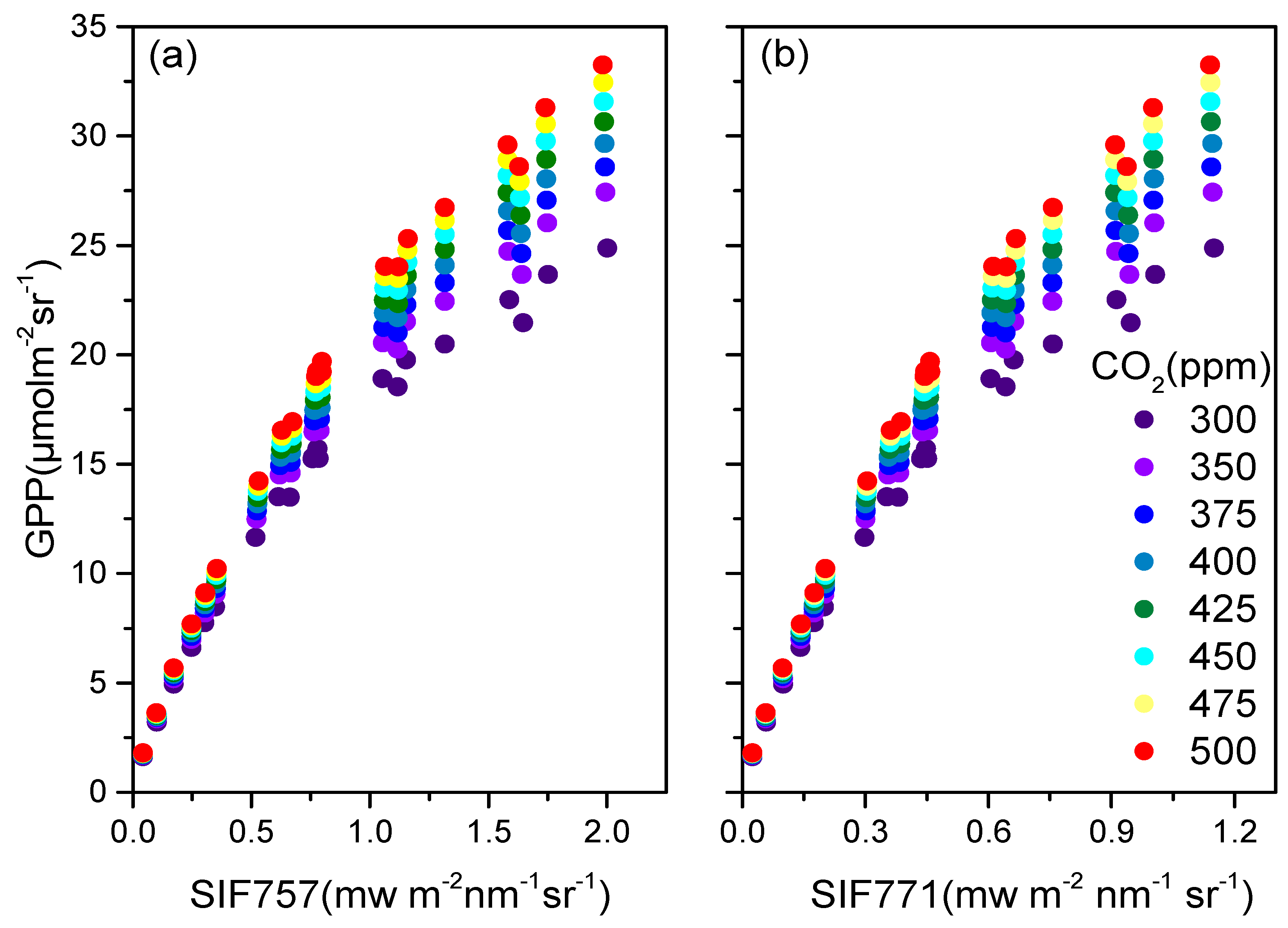
3.5. Mechanism of CO2 Affecting Modeling of GPP

Our results have shown that considering atmospheric CO2 concentrations can improve the accuracy of the GPP estimates. However, it is uncertain whether this improvement is statistically artificial or driven by real ecological processes. Therefore, we used the SCOPE model to explore the possible mechanisms behind the statistical results. SIF of two bands were included in this experiment. Figure 8 shows relationships between SIF and simulated GPP. To highlight the effect of the atmospheric CO2 concentration, each dot is colored according to its atmospheric CO2 concentration. Two main conclusions can be drawn from Figure 8. Firstly, there is a non-linear relationship between SIF and simulated GPP within half an hour. Current researchers usually applied an adjustment factor to convert instantaneous SIF to daily SIF, then built linear relationships with daily GPP. However, some researches have shown that the relationship between SIF and GPP could be non-linear. At present, there is no uniform conclusion as to whether SIF and GPP are linear or non-linear. Therefore, if we represent the nonlinear relationship in terms of linear relationship, it tends to lead to overestimation and underestimation of the GPP. The same phenomenon is shown in Figure 8. From Figure 7, we can conclude that CO2 corrects for the SIF-GPP linear model overestimating GPP in summer and fall and underestimating GPP in spring and winter. Therefore, adding CO2 to the SIF-GPP linear model may result in an equilibrium between the linear and non-linear relationship of SIF and GPP. Second, linear regression models are not sufficient to accurately link SIF and GPP when atmospheric CO2 concentrations change. It is clear that the simulated GPP at high CO2 concentrations is higher than that at low CO2 concentrations, and the higher the SIF intensity, the greater the difference in the simulated GPP at different CO2 concentrations, and the results of the SCOPE simulation are consistent with the previous statistical results. These results re-emphasize that the effects of atmospheric CO2 concentrations should be considered when modelling GPP using SIF as a key driver. A plausible explanation for this result is that atmospheric CO2 concentration is a key constraint on photosynthetic efficiency.
Photosynthesis consists of light reactions and dark reactions. Light reactions are chlorophyll’s conversion of light energy into electrical energy and then into active chemical energy, which is finally stored in ATP (ATP adenosine triphosphate). The essence of the dark reaction is the assimilation of CO2 to CH2O under the action of various enzymes in the chloroplast stroma. Therefore, CO2 is the main raw material for photosynthesis and an important factor affecting the intensity of photosynthetic. GPP is the amount of organic carbon fixed by green plants per unit area through photosynthesis per unit time. CO2 assimilation rate refers to the amount of dry matter added to plants per unit time and per unit assimilated area. If the CO2 assimilation rate increased, then the amount of fixed organic carbon per unit time would increase simultaneously.

4. Discussions

4.1. Reasons for Differences between SIF-GPP and SIF-CO2-GPP Model

Previous studies had shown that the atmospheric CO2 concentration is a non-negligible driving factor of GPP. The influence of the atmospheric CO2 concentration on ecosystems could even exceed the temperature and precipitation [41,42]. Under the environment of the surging atmospheric CO2 concentration, the photosynthesis of vegetation would be enhanced, which is the so-called CO2 fertilization effect [34]. When the CO2 concentration rises, the CO2 concentration between plant cells increases, which is the main factor affecting the photosynthetic rate of vegetation [43]. Therefore, the increase in the atmospheric CO2 concentration would effectively promote the improvement of ecosystem productivity. In the meantime, it is also illustrated that when the atmospheric CO2 concentration is elevated to a very high level, the photosynthesis of vegetation will be in turn reduced to the original efficiency [44,45,46]. Therefore, we believe it is necessary to consider the effects of atmospheric CO2 concentrations when trying to estimate GPP using SIF products as key driven factor. There is a significant seasonal change in CO2 in the forest, peaking before the spring and dropping to troughs at the end of the summer [35]. Figure 7a,e shows that GPPM is higher than GPPS in the spring, and we calculated the monthly average CO2 concentration for four selected months using in situ CO2 measurements from the US-PFa flux tower. The monthly surface average CO2 concentration of EC tower in April is 407.84 ppm, which is the second higher, second only to that in winter. Spring is often accompanied by a surge in CO2 concentration to promote the germination of vegetation. We speculate that SIF-GPP model does not take the atmospheric CO2 concentration into account and thus ignore the CO2 fertilization effect. That could explain why GPPM is higher than GPPS at this stage. Actually, the fact that the increasing CO2 concentration in a short term promotes photosynthesis of vegetation has been reported widely [30,47]. It is thus implied that the vegetation carbon sequestration capacity could be underestimated in spring if GPP was estimated using SIF data alone. Figure 7b,f shows that GPPM is lower than GPPS in summer. The monthly surface concentration is 402.25 ppm for June. The vegetation is lush, and daytime is long in summer. Strong photosynthesis in summer reduces CO2 concentration in the canopy to lower than that in the free atmosphere [35]. Relatively lower CO2 concentration inhibits the effect of vegetation photosynthesis [48]. That could explain why GPPM is lower than GPPS in summer. Figure 7c,g shows that GPPM is lower than GPPS in autumn. The monthly surface concentration is 401.52 ppm for September. The CO2 concentration in the early autumn is lower than that in summer. Low concentrations of CO2 and gradual deciduous vegetation reduce the photosynthetic rate of vegetation, limiting the fertilization effect of CO2. Therefore, the value of GPPM is lower compared with GPPS. The value of GPPM is closer to the measured GPP of the EC Flux Towers, which supports the above discussion to some extent. Figure 7d,h shows that the mean GPPM is higher than the mean GPPS in winter. In temperate forests, GPP should drop to an extremely low level in winter. The monthly surface CO2 concentration in November is 411.73 ppm. CO2 concentration increases rapidly during the winter. A surge in CO2 concentration promotes photosynthesis of vegetation [49]. That could partly explain why SIF-CO2-GPP model overestimate GPP comparing with the SIF-GPP model. Besides, there are several “hotspots” in the map of GPPS as shown in Figure 7h. We think that such “hotspots” could be wrong estimates. The SIF-CO2-GPP model corrects those “hotspots” in its results. We think that the homogeneous distribution of GPP with a very low value would be more in line with the growth state of vegetation in winter. Therefore, the SIF-CO2-GPP model also improves the accuracy of the SIF estimates for winter GPP. The inclusion of atmospheric CO2 concentrations in the model will significantly improve the accuracy of the estimates and better present the spatial distribution of the GPP.
Moreover, a reasonable mechanism to explain improvements brought by the SIF-CO2-GPP model can be expressed as follows. When the CO2 concentration at surface leaves increases, the value of the CO2 compensation point reduces and the carboxylation rate increases, which would increase the gross photosynthetic rate. Meanwhile, the respiration would be limited with the increasing the CO2 concentration, resulting in increasing in the net photosynthetic rate. Eventually, the GPP would become higher and vice versa. Looking back to Figure 7, we can see that comparing with the SIF-GPP model, the SIF-CO2-GPP model overestimated GPP in winter and underestimated GPP in summer. Such results are consistent with the above mechanism.

4.2. Uncertainties and Limitations

Though the proposed SIF-CO2-GPP model shows promising potentials to map GPP with a better accuracy, there are still several problems to be solved in the future to reach better performance. The uncertainty and limitation of the proposed method are mainly attributed to the following three aspects. First of all, although the spatial resolution of products of OCO-2 satellite is improved compared with other satellites, the footprint is still large compared with those of EC Flux Towers [18]. We demonstrate the footprint of OCO-2 SIF products on October 2014 in Figure 9. As can be seen from Figure 9, the spatial coverage of OCO-2 SIF products is relatively dense between 30°S and 30°N than those in high-latitude regions. That would hinder applications of the proposed method in high-latitude regions where boreal forests locate. Owing to the same reason, there would be a fraction of products of target mode, which would be inappropriate as an input of the proposed model. Even if we had tried our best to select research areas where the vegetation type is uniform, the coarse resolution could still lead to ignorance of heterogeneity in a single pixel, which would eventually reduce the reliability of GPP estimates. The fluorescence detector (Flex) is due to be launched around 2022, which will provide SIF products with finer resolution comparing with those of OCO-2. That would help reduce the error caused by the insufficient resolution of existing SIF products. Moreover, studies have shown that SIF saturates at a relatively low light intensity. This also affects the accuracy of using SIF to estimate GPP [50]. Secondly, the coverage of OCO-2 is sparser than that of MODIS, which results in limited observations for most EC flux towers. This is also a common disadvantage of estimating GPP using satellite-based SIF products with respect to LUE models. As a consequence, the probability of coincidences of the ground stations and the satellite footprints is significantly reduced due to the incomplete coverage of OCO-2. Tackling that problem, we have to lower the criteria for judging coincidences of EC flux towers and SIF products of OCO-2 in this study. Then, such spatial mismatch leads to inevitable errors in SIF, which is the key input of the GPP-estimating model and eventually propagates to estimates of GPP. Consequently, it is of great significance to develop some combined methods to complement the advantages of two different categories of models, namely, SIF-driven models and LUE models. Finally, the SIF data observed in the Target mode is evidently affected by VZA, but in this study, we did not consider this factor. Moreover, we realized that when processing SIF data, the SIF value near 0 should be retained to ensure the accuracy of the experimental results because of the error of the SIF retrieve algorithm. In addition, the impact of CO2 on vegetation is complex, closely related to the growth state of vegetation and the type of vegetation, which calls for further research in the field of botany.
This study is a tentative exploration on estimating GPP using XCO2 and SIF products of OCO-2, due to the limited number of accessible EC flux towers. In future works, we are going to further improve the SIF-CO2-GPP model using products of more EC flux towers to realize mapping of GPP globally with higher accuracy.

5. Conclusions

The SIF product becomes the emerging proxy to estimate GPP with a higher accuracy globally along with the launch of OCO-2. Moreover, several previous studies in the field of botany had mentioned that the atmospheric CO2 concentration is a critical factor in determining the photosynthesis efficiency. In this study, we proposed a SIF-CO2-GPP model to take the effect of the atmospheric CO2 concentration on photosynthesis into considerations of estimating GPP, aiming at better modeling of GPP by means of satellite products. This study confirms that the effect of atmospheric CO2 concentrations on the photosynthesis efficiency can be also observed at a larger spatial scale, which is a promising feature to estimate GPP using remotely sensed products. Our results showed that the SIF-CO2-GPP linear model (R2 = 0.63 − 0.90, p < 0.001) is more suitable to estimate GPP comparing with the linear SIF-GPP model (R2 = 0.41 − 0.87, p < 0.001). In addition, the concentration of CO2 in the surface atmosphere is one of the key factors affecting GPP because it is the raw material for photosynthesis. We use the SCOPE model to prove that the atmospheric CO2 concentration is a factor affecting the modeling of GPP. A reasonable mechanism could be that the increment of CO2 concentration at leave’s surface would induce intercellular CO2 concentration and the CO2 assimilation rate raise. That eventually would cause a rise of GPP and vice versa. Moreover, there is a strongly linear relationship between XCO2 of OCO-2 and surface CO2 mixing ratio of EC Flux towers (R = 0.54 − 0.87, p < 0.001), laying the foundation for utilizing the SIF-CO2-GPP model to monitor global distributions of GPP using OCO-2 or other similar satellites. The availability of intensive OCO-2 products surrounding the US-PFa site allows us to generate grid SIF and XCO2 and then to estimate gridded GPP at the landscape scale for different seasons using SIF-CO2-GPP model and SIF-GPP model. Taking results of the SIF-CO2-GPP model as a benchmark, the traditional SIF-GPP model underestimates GPP in spring and winter and overestimates GPP in summer and autumn. Besides, we also confirmed that daily SIF is more suitable for estimating GPP than instantaneous SIF. In addition, SIF757 is also more strongly correlated with GPP than SIF771 for most forests. In future works, investigations on relationships among SIF, XCO2 and GPP should be deepened for more vegetation types and more latitude zones after obtaining more in situ measurements of EC flux towers. Furthermore, along with forthcoming products from GOSAT-3, OCO-3 and FLEX, we believe that the SIF-CO2-GPP model would help obtain accurate GPP estimates with high spatial resolution and large coverage, providing better data and new prospects for climate change and carbon cycle studies.

Author Contributions

Conceptualization, R.Q. and G.H.; methodology, R.Q. and G.H.; software, R.Q.; validation, R.Q.; writing—original draft preparation, R.Q. and G.H.; writing—review and editing, R.Q., G.H., X.M., H.X., T.S. and M.Z. Investigation, Z.S. and H.X.; Resources, Z.S. and M.Z. All authors have read and agreed to the published version of the manuscript.

Funding

This work was supported by the National Natural Science Foundation of China (Grant No. 41971283, 41801261, 41827801, 41801282), the National Key Research and Development Program of China (2017YFC0212600), Postdoctoral Science Foundation of China (2017T100580).

Acknowledgments

We thank the OCO-2 and Ameriflux teams for making the SIF and GPP data.

Conflicts of Interest

The authors declare no conflict of interest.

References

  1. Piao, S.; Sitch, S.; Ciais, P.; Friedlingstein, P.; Peylin, P.; Wang, X.; Ahlstrom, A.; Anav, A.; Canadell, J.G.; Cong, N.; et al. Evaluation of terrestrial carbon cycle models for their response to climate variability and to CO2 trends. Glob. Chang. Biol. 2013, 19, 2117–2132. [Google Scholar] [CrossRef] [PubMed] [Green Version]
  2. Watson, A.J.; Schuster, U.; Bakker, D.C.E.; Bates, N.R.; Corbiere, A.; Gonzalez-Devila, M.; Friedrich, T.; Hauck, J.; Heinze, C.; Johannessen, T.; et al. Tracking the Variable North Atlantic Sink for Atmospheric CO2. Science 2009, 326, 1391–1393. [Google Scholar] [CrossRef] [PubMed]
  3. Joeri, R.; McCollum, D.L.; Andy, R.; Malte, M.; Keywan, R. Probabilistic cost estimates for climate change mitigation. Nature 2013, 493, 79–83. [Google Scholar]
  4. Markus, R.; Michael, B.; Philippe, C.; Dorothea, F.; Mahecha, M.D.; Seneviratne, S.I.; Jakob, Z.; Christian, B.; Nina, B.; Frank, D.C. Climate extremes and the carbon cycle. Nature 2013, 500, 287–295. [Google Scholar]
  5. Schimel, D.; Pavlick, R.; Fisher, J.B.; Asner, G.P.; Saatchi, S.; Townsend, P.; Miller, C.; Frankenberg, C.; Hibbard, K.; Cox, P. Observing terrestrial ecosystems and the carbon cycle from space. Glob. Chang. Biol. 2015, 21, 1762–1776. [Google Scholar] [CrossRef]
  6. Amiro, B.D.; Barr, A.G.; Barr, J.G.; Black, T.A.; Bracho, R.; Brown, M.; Chen, J.; Clark, K.L.; Davis, K.J.; Desai, A.R.; et al. Ecosystem carbon dioxide fluxes after disturbance in forests of North America. J. Geophys. Res. Biogeosci. 2010, 115, 458–471. [Google Scholar] [CrossRef]
  7. Gebremichael, M.; Barros, A.P. Evaluation of MODIS gross primary productivity (GPP) in tropical monsoon regions. Remote Sens. Environ. 2006, 100, 150–166. [Google Scholar] [CrossRef]
  8. Joiner, J.; Guanter, L.; Lindstrot, R.; Voigt, M.; Vasilkov, A.P.; Middleton, E.M.; Huemmrich, K.F.; Yoshida, Y.; Frankenberg, C. Global monitoring of terrestrial chlorophyll fluorescence from moderate-spectral-resolution near-infrared satellite measurements: Methodology, simulations, and application to GOME-2. Atmos. Meas. Tech. 2013, 6, 2803–2823. [Google Scholar] [CrossRef] [Green Version]
  9. Verma, M.; Schimel, D.; Evans, B.; Frankenberg, C.; Beringer, J.; Drewry, D.T.; Magney, T.; Marang, I.; Hutley, L.; Moore, C. Effect of environmental conditions on the relationship between solar-induced fluorescence and gross primary productivity at an OzFlux grassland site. J. Geophys. Res. Biogeosci. 2017, 122, 716–733. [Google Scholar] [CrossRef] [Green Version]
  10. Yang, H.; Yang, X.; Zhang, Y.; Heskel, M.A.; Lu, X.; Munger, J.W.; Sun, S.; Tang, J. Chlorophyll fluorescence tracks seasonal variations of photosynthesis from leaf to canopy in a temperate forest. Glob. Chang. Biol. 2017, 23, 2874–2886. [Google Scholar] [CrossRef]
  11. Yang, X.; Tang, J.; Mustard, J.F.; Lee, J.E.; Rossini, M.; Joiner, J.; Munger, J.W.; Kornfeld, A.; Richardson, A.D. Solar-induced chlorophyll fluorescence that correlates with canopy photosynthesis on diurnal and seasonal scales in a temperate deciduous forest. Geophys. Res. Lett. 2015, 42, 2977–2987. [Google Scholar] [CrossRef]
  12. Li, X.; Xiao, J.; He, B. Chlorophyll fluorescence observed by OCO-2 is strongly related to gross primary productivity estimated from flux towers in temperate forests. Remote Sens. Environ. 2018, 204, 659–671. [Google Scholar] [CrossRef]
  13. Liu, X.; Guanter, L.; Liu, L.; Damm, A.; Malenovský, Z.; Rascher, U.; Peng, D.; Du, S.; Gastellu-Etchegorry, J.P. Downscaling of solar-induced chlorophyll fluorescence from canopy level to photosystem level using a random forest model. Remote Sens. Environ. 2018, 231, 359–371. [Google Scholar] [CrossRef]
  14. Ahl, D.E.; Gower, S.T.; Mackay, D.S.; Burrowsa, S.N.; Normanc, J.M.; Diakd, G.R. The effects of aggregated land cover data on estimating NPP in northern Wisconsin. Remote Sens. Environ. 2005, 97, 1–14. [Google Scholar] [CrossRef]
  15. Zhao, M.; Running, S.W.; Nemani, R.R. Sensitivity of Moderate Resolution Imaging Spectroradiometer (MODIS) terrestrial primary production to the accuracy of meteorological reanalyses. J. Geophys. Res. Space Phys. 2006, 111, 14–28. [Google Scholar] [CrossRef] [Green Version]
  16. Frankenberg, C.; Butz, A.; Toon, G.C. Disentangling chlorophyll fluorescence from atmospheric scattering effects in O-2 A-band spectra of reflected sun-light. Geophys. Res. Lett. 2011, 38, 149–157. [Google Scholar] [CrossRef]
  17. Guanter, L.; Frankenberg, C.; Dudhia, A.; Lewis, P.E.; Gómez-Dans, J.; Kuze, A.; Suto, H.; Grainger, R.G. Retrieval and global assessment of terrestrial chlorophyll fluorescence from GOSAT space measurements. Remote Sens. Environ. 2012, 121, 236–251. [Google Scholar] [CrossRef]
  18. Li, X.; Xiao, J.; He, B.; Altaf Arain, M.; Beringer, J.; Desai, A.R.; Emmel, C.; Hollinger, D.Y.; Krasnova, A.; Mammarella, I.; et al. Solar-induced chlorophyll fluorescence is strongly correlated with terrestrial photosynthesis for a wide variety of biomes: First global analysis based on OCO-2 and flux tower observations. Glob. Chang. Biol. 2018, 24, 3990–4008. [Google Scholar] [CrossRef]
  19. Zarco-Tejada, P.J.; Morales, A.; Testi, L.; Villalobos, F.J. Spatio-temporal patterns of chlorophyll fluorescence and physiological and structural indices acquired from hyperspectral imagery as compared with carbon fluxes measured with eddy covariance. Remote Sens. Environ. 2013, 133, 102–115. [Google Scholar] [CrossRef]
  20. Croft, H.; Chen, J.M.; Luo, X.; Bartlett, P.; Chen, B.; Staebler, R.M. Leaf chlorophyll content as a proxy for leaf photosynthetic capacity. Glob. Chang. Biol. 2017, 23, 3513–3524. [Google Scholar] [CrossRef]
  21. Zhang, Y.; Guanter, L.; Berry, J.A.; Joiner, J.; van der Tol, C.; Huete, A.; Gitelson, A.; Voigt, M.; Kohler, P. Estimation of vegetation photosynthetic capacity from space-based measurements of chlorophyll fluorescence for terrestrial biosphere models. Glob. Chang. Boil. 2014, 20, 3727–3742. [Google Scholar] [CrossRef] [PubMed] [Green Version]
  22. Sun, Y.; Frankenberg, C.; Jung, M.; Joiner, J.; Guanter, L.; Kohler, P.; Magney, T. Overview of Solar-Induced chlorophyll Fluorescence (SIF) from the Orbiting Carbon Observatory-2: Retrieval, cross-mission comparison, and global monitoring for GPP. Remote Sens. Environ. 2018, 209, 808–823. [Google Scholar] [CrossRef]
  23. Chatterjee, A.; Gierach, M.M.; Sutton, A.J.; Feely, R.A.; Crisp, D.; Eldering, A.; Gunson, M.R.; O’Dell, C.W.; Stephens, B.B.; Schimel, D.S. Influence of El Nino on atmospheric CO2 over the tropical Pacific Ocean: Findings from NASA’s OCO-2 mission. Science 2017, 358, 27–39. [Google Scholar] [CrossRef] [PubMed] [Green Version]
  24. Kohler, P.; Guanter, L.; Joiner, J. A linear method for the retrieval of sun-induced chlorophyll fluorescence from GOME-2 and SCIAMACHY data. Atmos. Meas. Tech. 2015, 8, 2589–2608. [Google Scholar] [CrossRef] [Green Version]
  25. Yang, X.; Tang, J.; Mustard, J.F.; Wu, J.; Zhao, K.; Serbin, S.; Lee, J.E. Seasonal variability of multiple leaf traits captured by leaf spectroscopy at two temperate deciduous forests. Remote Sens. Environ. 2016, 179, 1–12. [Google Scholar] [CrossRef] [Green Version]
  26. Zhang, Y.G.; Guanter, L.; Berry, J.A.; van der Tol, C.; Yang, X.; Tang, J.W.; Zhang, F.M. Model-based analysis of the relationship between sun-induced chlorophyll fluorescence and gross primary production for remote sensing applications. Remote Sens. Environ. 2016, 187, 145–155. [Google Scholar] [CrossRef] [Green Version]
  27. Zhang, Z.; Zhang, Y.; Joiner, J.; Migliavacca, M. Angle matters: Bidirectional effects impact the slope of relationship between gross primary productivity and sun-induced chlorophyll fluorescence from Orbiting Carbon Observatory-2 across biomes. Glob. Chang. Biol. 2018, 24, 5017–5020. [Google Scholar] [CrossRef] [Green Version]
  28. Walker, A.P.; De Kauwe, M.G.; Medlyn, B.E.; Zaehle, S.; Iversen, C.M.; Asao, S.; Guenet, B.; Harper, A.; Hickler, T.; Hungate, B.A.; et al. Decadal biomass increment in early secondary succession woody ecosystems is increased by CO2 enrichment. Nat. Commun. 2019, 10, 587–599. [Google Scholar] [CrossRef]
  29. Kitaya, Y.; Shibuya, T.; Yoshida, M.; Kiyota, M. Effects of air velocity on photosynthesis of plant canopies under elevated CO levels in a plant culture system. Adv. Space Res. Off. J. Comm. Space Res. 2004, 34, 1466–1469. [Google Scholar] [CrossRef]
  30. Jones, A.G.; Scullion, J.; Ostle, N.; Levy, P.E.; Gwynn-Jones, D. Completing the FACE of elevated CO2 research. Environ. Int. 2014, 73, 252–258. [Google Scholar] [CrossRef] [Green Version]
  31. Wenzel, S.; Cox, P.M.; Eyring, V.; Friedlingstein, P. Projected land photosynthesis constrained by changes in the seasonal cycle of atmospheric CO2. Nature 2016, 538, 195–208. [Google Scholar] [CrossRef] [PubMed]
  32. Winkler, A.J.; Myneni, R.B.; Alexandrov, G.A.; Brovkin, V. Earth system models underestimate carbon fixation by plants in the high latitudes. Nat. Commun. 2019, 10, 224–235. [Google Scholar] [CrossRef] [PubMed]
  33. Mizoguchi, Y.; Ohtani, Y.; Takanashi, S.; Iwata, H.; Yasuda, Y.; Nakai, Y. Seasonal and interannual variation in net ecosystem production of an evergreen needleleaf forest in Japan. J. For. Res. 2012, 17, 283–295. [Google Scholar] [CrossRef]
  34. Los, S.O. Analysis of trends in fused AVHRR and MODIS NDVI data for 1982–2006: Indication for a CO2 fertilization effect in global vegetation. Glob. Biogeochem. Cycles 2013, 27, 318–330. [Google Scholar] [CrossRef]
  35. Murayama, S.; Saigusa, N.; Chan, D.; Yamamoto, S.; Kondo, H.; Eguchi, Y. Temporal variations of atmospheric CO2 concentration in a temperate deciduous forest in central Japan. Tellus Ser. B-Chem. Phys. Meteorol. 2003, 55, 232–243. [Google Scholar] [CrossRef]
  36. Van der Tol, C.; Verhoef, W.; Rosema, A. A model for chlorophyll fluorescence and photosynthesis at leaf scale. Agric. For. Meteorol. 2009, 149, 96–105. [Google Scholar] [CrossRef]
  37. Van der Tol, C.; Verhoef, W.; Timmermans, J.; Verhoef, A.; Su, Z. An integrated model of soil-canopy spectral radiances, photosynthesis, fluorescence, temperature and energy balance. Biogeosciences 2009, 6, 3109–3129. [Google Scholar] [CrossRef] [Green Version]
  38. Kothavala, Z.; Arain, M.A.; Black, T.A.; Verseghy, D. The simulation of energy, water vapor and carbon dioxide fluxes over common crops by the Canadian Land Surface Scheme (CLASS). Agric. For. Meteorol. 2005, 133, 89–108. [Google Scholar] [CrossRef]
  39. Xu, L.; Baldocchi, D.D. Seasonal trends in photosynthetic parameters and stomatal conductance of blue oak (Quercus douglasii) under prolonged summer drought and high temperature. Tree Physiol. 2003, 23, 865–877. [Google Scholar] [CrossRef] [Green Version]
  40. Verrelst, J.; Tol, C.V.D.; Magnani, F.; Sabater, N.; Rivera, J.P.; Mohammed, G.; Moreno, J. Evaluating the predictive power of sun-induced chlorophyll fluorescence to estimate net photosynthesis of vegetation canopies: A SCOPE modeling study. Remote Sens. Environ. 2016, 176, 139–151. [Google Scholar] [CrossRef]
  41. Cramer, W.; Bondeau, A.; Woodward, F.I.; Prentice, I.C.; Betts, R.A.; Brovkin, V.; Cox, P.M.; Fisher, V.; Foley, J.A.; Kucharik, C.; et al. Global response of terrestrial ecosystem structure and function to CO2 and climate change: Results from six dynamic global vegetation models. Glob. Chang. Biol. 2010, 7, 357–373. [Google Scholar] [CrossRef] [Green Version]
  42. Sun, Y.; Frankenberg, C.; Wood, J.D.; Schimel, D.S.; Jung, M.; Guanter, L.; Drewry, D.; Verma, M.; Porcar-Castell, A.; Griffis, T.J.; et al. OCO-2 advances photosynthesis observation from space via solar-induced chlorophyll fluorescence. Science 2017, 358, 258–267. [Google Scholar] [CrossRef] [PubMed] [Green Version]
  43. Li, H.M.; He, X.Y.; Wang, K.L. and Chen, W. Photosynthetic characteristics of five arbor species in Shenyang urban area. Chin. J. Appl. Ecol. 2007, 18, 1709–1714. [Google Scholar]
  44. Frankenberg, C.; O’Dell, C.; Berry, J.; Guanter, L.; Joiner, J. Prospects for chlorophyll fluorescence remote sensing from the Orbiting Carbon Observatory-2. Remote Sens. Environ. 2014, 147, 1–12. [Google Scholar] [CrossRef] [Green Version]
  45. Johnson, D.W. Progressive N limitation in forests: Review and implications for long-term responses to elevated CO2. Ecology 2006, 87, 64–75. [Google Scholar] [CrossRef] [PubMed] [Green Version]
  46. Luo, Y.; Su, B.; Currie, W.J.; Finzi, A.; Hartwig, U.; Hungate, B.; McMurtrie, R.; Oren, R.; Parton, W. Progressive nitrogen limitation of ecosystem responses to rising atmospheric carbon dioxide. Bioscience 2004, 54, 731–739. [Google Scholar] [CrossRef] [Green Version]
  47. Ainsworth, E.A.; Rogers, A. The response of photosynthesis and stomatal conductance to rising [CO2]: Mechanisms and environmental interactions. Plant Cell Environ. 2010, 30, 258–270. [Google Scholar] [CrossRef]
  48. Von Caemmerer, S.; Quick, W.P. and Furbank, R.T. The development of C4 rice: Current progress and future challenges. Science 2012, 336, 1671. [Google Scholar] [CrossRef]
  49. Friedlingstein, P.; Cox, P.; Betts, R.; Bopp, L.; von Bloh, W.; Brovkin, V.; Cadule, P.; Doney, S.; Eby, M.; Fung, I.; et al. Climate–Carbon Cycle Feedback Analysis: Results from the C4MIP Model Intercomparison. J. Clim. 2006, 19, 3337. [Google Scholar] [CrossRef]
  50. Soukupová, J.; Cséfalvay, L.; Urban, O.; Košvancová, M.; Marek, M.; Rascher, U.; Nedbal, L. Annual variation of the steady-state chlorophyll fluorescence emission of evergreen plants in temperate zone. Funct. Plant Biol. 2008, 35, 63–76. [Google Scholar] [CrossRef]
Figure 1. Location and attribute of selected EC sites. (a) An enlarged image showing sites of US-PFa, US-Syv, US-WCr, US-Los and US-Ro4. (b) An enlarged image showing sites of CA-TP3, CA-TP4 and TPD. (c) The location map of the study area; the five-pointed star indicates the location of the study area, and the base map is created in ARCGIS using MCD12Q1 data.
Remotesensing 12 01377 g001
Figure 2. The flow diagram of this study.
Remotesensing 12 01377 g002
Figure 3. The linear relationship between instantaneous solar-induced chlorophyll fluorescence (SIF) and instantaneous gross primary productivity (GPP) for different EC flux towers. The red circle represents the data of ins757 while the black dot represents the data of ins771. The linear relationships are presented in colorful lines for different independent variables.
Remotesensing 12 01377 g003
Figure 4. The linear relationship between daily SIF and daily GPP for different EC flux towers. The red circle represents the data of daily757 while the black dot represents the data of daily771. The linear relationships are presented in colorful lines for different independent variables.
Remotesensing 12 01377 g004
Figure 5. Validation of the SIF-GPP model and the SIF-CO2-GPP model for different EC flux towers. The black dots represent the GPP estimated by the SIF-CO2-GPP model, and the red circles represent the GPP estimated by the SIF-GPP model. The fit lines for GPP of the flux towers and GPPM are indicated by black lines. Fitting lines for GPP for flux towers and GPPS are indicated by red lines.
Remotesensing 12 01377 g005
Figure 6. Linear relationships between XCO2 of OCO-2 and measured surface CO2 mixing ratio of EC flux towers. Dots indicate CO2 of EC towers and XCO2 fit points at the flux towers, and black lines indicate the fit line.
Remotesensing 12 01377 g006
Figure 7. Gridded GPP estimated by means of the SIF-CO2-GPP model for four seasons, (a)–(d). Gridded GPP estimated by means of SIF- GPP model for four seasons, (e)–(h). The value underneath the date represents the mean modeled GPP data in selected regions and the unit of GPP is g C m−2d−1.
Remotesensing 12 01377 g007
Figure 8. Sensitivity analysis of the effects of different levels of atmospheric CO2 concentrations on SIF-GPP relationship. (a) SIF757 versus GPP; (b) SIF771 versus GPP.
Remotesensing 12 01377 g008
Figure 9. The spatial coverage of the OCO-2 satellite in October 2014; the color of the footprint indicates the magnitude of the chlorophyll fluorescence value, yellow indicates a high value and blue indicates a low value.
Remotesensing 12 01377 g009
Table 1. Detailed information of eddy covariance (EC) Flux Towers, including site’s name, latitude, longitude, the year of data used and its institution (ENF: Evergreen Needleleaf Forests, DBF: Deciduous Broadleaf Forests, GRA: Grasslands, OSH: Open shrublands, MF: Mixed Forest, WET: Permeland Wetlands).
SiteLat (°)Lon (°)YearTypeInstitution
CA-TP342.71−80.352014–2017ENFMcMaster University
CA-TP442.71−80.362014–2017ENFMcMaster University
US-Los46.09−89.982014–2019WETUniversity of Wisconsin
CA-TPD42.64−80.562014–2015DBFMcMaster University
US-Srr38.20−122.032014–2017WETUSGS
US-Syv46.24−89.352014–2018MFUniversity of Wisconsin
US-PFa45.95−90.272014–2018MFUniversity of Wisconsin
US-SCC61.31−121.302014–2016ENFUniversity of California
US-EML63.88−149.252014–2018OSHUniversity of Northern Arizona
US-Ro444.68−122.032014–2019GRAUSDA-ARS
US-PHM42.47−70.832014–2018WETMarine Biological Laboratory
US-WCr45.81−90.272014–2018DBFUniversity of Wisconsin
Table 2. Comparisons of R2 of SIF-GPP models at instantaneous and daily scales.
Siteins757-GPPDaily757-GPP
US-Srr0.30 (p < 0.001)0.53 (p < 0.001)
US-WCr0.67 (p < 0.001)0.80 (p < 0.001)
US-Syv0.18 (p < 0.001)0.61 (p < 0.001)
US-PFa0.60 (p < 0.001)0.72 (p < 0.001)
CA-TP30.40 (p < 0.001)0.47 (p < 0.001)
CA-TP40.47 (p < 0.001)0.41 (p < 0.001)
CA-SCC0.74 (p < 0.001)0.68 (p < 0.001)
US-EML0.81 (p < 0.001)0.73 (p < 0.001)
US-PHM0.60 (p < 0.001)0.75 (p < 0.001)
US-Ro40.74 (p < 0.001)0.87 (p < 0.001)
US-TPD0.36 (p < 0.001)0.40 (p < 0.001)
US-Los0.81 (p < 0.001)0.64 (p < 0.001)
Table 3. Comparison of the SIF-GPP model and the SIF-CO2-GPP model. Increase rate is the difference between the R2 of both models. The CO2 data comes from the EC flux tower.
SiteSIF-GPP ModelSIF-CO2-GPP ModelIncrease Rate
(%)
Fitted FormulaR2Fitted FormulaR2
US-SrrGPP = 44.97 * × SIF − 2.670.53GPP = 11.52 × SIF − 0.16 × CO2 + 65.370.7032%
US-WCrGPP = 21.06 × SIF − 1.780.80GPP = 19.80 × SIF − 0.05 × CO2 + 18.490.834%
US-SyvGPP = 20.50 × SIF + 1.980.61GPP = 9.37 × SIF − 0.53 × CO2 + 214.290.8641%
US-PFaGPP = 15.86 × SIF − 0.640.72GPP = 11.52 × SIF − 0.16 × CO2 + 65.370.8819%
US-TP3GPP = 30.05 × SIF + 2.970.47GPP = 29.42 × SIF − 0.41 × CO2 + 150.730.6334%
US-TP4GPP = 29.20 × SIF + 2.900.41GPP = 9.42 × SIF − 0.47 × CO2 + 179.320.6733%
CA-SCCGPP = 42.70 × SIF − 0.800.68GPP = 33.81 × SIF − 0.05 × CO2 + 22.640.737%
US-EMLGPP = 18.56 × SIF + 0.730.73GPP = 23.48 × SIF + 0.07 × CO2 − 27.530.8010%
US-TPDGPP = 27.70 × SIF + 7.020.40GPP = 32.30 × SIF + 0.11 × CO2 − 37.610.5025%
US-Ro4GPP = 42.92 × SIF − 1.090.87GPP = 49.09 × SIF + 0.08 × CO2 − 36.030.903%
US-PHMGPP = 17.82 × SIF − 0.640.75GPP = 17.74 × SIF − 0.001 × CO2 − 0.400.773%
US-LosGPP = 8.77 × SIF − 0.010.64GPP = 8.256 × SIF − 0.07 × CO2 + 29.570.699%
Table 4. Root-mean-square error (RMSE) of SIF-GPP and SIF-CO2-GPP model. The unit is g Cm−2 day−1.
SitesSIF-GPPSIF-CO2-GPP
US-Srr 2.371.80
US-WCr1.721.71
US-Syv1.861.86
US-PFa1.511.20
CA-TP32.401.87
CA-TP42.891.28
CA-SCC2.091.45
US-EML2.111.26
US-PHM1.211.23
US-Ro42.432.45
US-TPD3.092.79
US-Los2.742.80

