Remote Sensing-Based Mapping of Senescent Leaf C:N Ratio in the Sundarbans Reserved Forest Using Machine Learning Techniques

Abstract

Carbon to nitrogen ratio (C:N) of senescent leaf is a crucial functional trait and indicator of litter quality that affects belowground carbon and nitrogen cycles, especially soil decomposition. Although mapping the C:N ratio of fresh mature canopies has been attempted, few studies have attempted to map the C:N ratio of senescent leaves, particularly in mangroves. In this study, four machine learning models (Stochastic Gradient Boosting, SGB; Random Forest, RF; Support Vector Machine, SVM; and Partial Least Square Regression, PLSR) were compared for testing the predictability of using the Landsat TM 5 (LTM5) and Landsat 8 to map spatial and temporal distribution of C:N ratio of senescent leaves in Sundarbans Reserved Forest (SRF), Bangladesh. Surface reflectance of bands, texture metrics of bands and vegetation indices of LTM5 and Landsat 8 yearly composite images were extracted using Google Earth Engine for 2009–2010 and 2019. We found SGB, RF and SVM were significant different from PLSR based on MAE, RMSE, and R² (p < 0.05). Our results indicate that remote sensing data, such as Landsat TM data, can be used to map the C:N ratio of senescent leaves in mangroves with reasonable accuracy. We also found that the mangroves had a high spatial variation of C:N ratio and the C:N ratio map developed in the current study can be used for improving the biogeochemical and ecosystem models in the mangroves.

1. Introduction

Mangroves grow in the intertidal zone of tropical and subtropical countries, are highly productive and have huge carbon sequestration capacity, especially into sediments [1,2]. Thus, mangroves play a tremendous role in climate regulation. For sustaining productivity and carbon sequestration, the nutrient cycling needs to be maintained [3,4]. Through litter decomposition, a keystone ecosystem process, the nutrient supply is maintained in mangrove forests, which is essential for plant growth [3,5,6,7,8]. Leaf litter quality such as carbon to nitrogen (C:N) ratio is often regarded as the key determinant of litter decomposition [3,5,6,7,8]. Litter quality also influences the activities of soil microorganisms that play the direct role in litter decomposition [7,9,10,11]. For example, poor litter quality (higher C:N ratio) with lower amount of labile C with higher amount of tannin content causes microbial immobilization [8,9,12]. In a forest ecosystem, litter mostly comes from the falling of senescent leaves [7,13]. The variability of C:N ratio in senescent leaves largely depends on species at community and ecosystem scale and on temperature and rainfall at large scale [9,12,14,15]. In mangrove, to a large extent, for instance, in Sundarbans Reserved Forest, species distribution follows hydrological gradients in terms of salinity and fresh water flow that might be influenced by the balance of C:N ratio and thereby nutrient cycling and primary productivity [7,16,17,18].

Furthermore, mangrove forest faces tremendous disturbances both human mediated and natural such as upstream fresh water harvest, deforestation, sea level rise, salt intrusion, temperature change and tropical cyclone [3,19,20,21]. Due to those disturbances the mangrove is altered by reducing sedimentation, increasing salinity, and changes in species composition. For example, the fast-growing salt-intolerant species are replaced by the slowly growing salt-tolerant species [3,19,20,21]. Consequently, these changes in environmental factors and species composition have altered leaf C:N ratio and thereby affected nutrient cycling and primary productivity of the ecosystem [3,16,22]. Therefore, mapping the spatial and temporal variation of C:N ratio is necessary for monitoring nutrient dynamics, forest productivity, and soil carbon cycles in the mangrove forests. In spatial and temporal context, remote sensing-based upscaling of C:N with in situ data is feasible in terms of logistic supports, time, inaccessibility, and periodic monitoring [22,23].

Of the different dimensions of plant diversity, the trait based diversity (functional diversity) has been regarded as the main driver of ecosystem services and function [24] because it has a mechanistic relationship with plant productivity and other ecosystem functions such as microbial litter decomposition and nutrient cycling [25]. Functional diversity is defined as the variation, range and value of functional traits in a given community [24,26,27]. It has been suggested that the stand level biogeochemistry is largely driven by the community weighted mean of trait value of dominant species (usually weighted by species relative basal area or abundance at plot or stand) [24,25,28]. For example, community weighted mean of leaf C:N, C, N determines forest biomass [29], productivity [25], forest growth [30], and litter decomposition [31,32]. Thus, scientists have used this plot level community weighted mean of trait value as a bridge between field based trait value with remote sensing properties for scaling up ecosystem level from regional to global scale in terrestrial ecosystems [23,25,33].

The optical remote sensing-based approach has been proven a practical, cost-effective and accurate way to upscale the plot based in situ foliar trait value to forest landscape level in terrestrial forest ecosystems [34,35,36]. For example, Walis et al. [34] used Landsat 8 for leaf toughness, specific leaf area, foliar N concentration, and foliar P concentration in the tropical montane forest. Another open-access remote satellite imagery is Sentinel 2, which has been used recently in foliar chemical and morphological properties such as N [37] mass per area, chlorophyll (Cab), N and carbon content [38]. Those studies mainly focused on different traits of green leaf in forest ecosystems, but application of open source satellite imagery in assessing the senescent leaf C:N as a litter quality is limited. The reason may be the inability of remote sensing to capture the senescent leaf spectral properties as old leaves are not present in upper canopy [35,39]. However, the stoichiometric studies showed that there is high correlation between green and senescent leaves C:N in forest, which may allow us to map C:N ratio of senescence by means of multispectral remote sensing [40,41,42].

Furthermore, the above mention studies used mainly spectral reflectance and texture (Grey Level Co-occurrence Matrices, GLCM) properties of different bands and normalized vegetation indices. The drawback of normalized vegetation indices is that it has a saturation effect over dense canopy that leads to poor accuracy in model validation and mapping of biophysical and biogeochemical canopy properties [35,43]. Along with texture and vegetation indices, the canopy moisture, water (Modified Normalized Difference water index; MNDWI), Disease Water Stress Indices (DWSI), thermal band (B6 of Landsat) can be used to improve model accuracy as functional traits vary with environmental factors and community composition [23,33,35,39,44]. In addition, other simple ratios between Visible, NIR (Near Infra-Red) and SWIR (Short-wave infra-red) bands, such as B3/B1, B5/B7, and B7/B2, that are sensitive to moisture content and forest vigor may also contribute to improving the accuracy of C:N ratio mapping [33,35,39,44].

Remote sensing-based modeling of functional traits in forest ecosystems has been followed by both parametric and non-parametric advance machine learning regression approaches [23,34,37,38,45]. The advantage of non-parametric machine learning over parametric modeling approaches such as multiple linear modeling is that it can handle both multicollinearity between predictors and noisy data with efficiency in selecting the key predictor from a large amount of predictors [46,47,48,49]. Moreno-Martínez et al. [23] reported the outperformance of Random Forest (RF) modeling technique over multiple linear model, neural networks, Kernel Ridge Regression, and Gaussian Process Regression in mapping leaf functional trait in terrestrial forests at the global scale. Similarly, Gara et al. [38] and Chumura et al. [37] mapped leaf N and C concentration accurately with RF. On the other hand, the application of two other machine learning modeling techniques, support vector machines (SVM) and artificial neural networks, in modeling N and C concentrations over intact and fragmented forest ecosystems have been found to have equal performance [45]. Another ensemble of learning regression method is Stochastic Gradient Boosting (SGB), which can deal with plenty of data and combine important predictors along with average predictors for strong perdition of dependent variable. It found an outperformance of RF in other forestry field (biomass mapping) [50]. However, application of SGB in functional trait such as C:N modeling and mapping is not well known.

In this study, to our current knowledge, for the first time in the mangrove ecosystem, we tested four machine learning models to map the spatial and temporal distribution of the community weighted mean of C:N of senescent in the Sundarbans Reserved Forest in Bangladesh using Landsat TM 5 and Landsat 8. Advanced remote sensing-based modeling approach (machine learning) can contribute in assessing the essential biodiversity variables for biodiversity target achievement (e.g., National Biodiversity Strategies and Action Plans related to Aichi Biodiversity Target 2020) [51]. Particularly, in remote sensing-based forest biochemical properties (C:N as an indicator of decomposition), monitoring and information systems can improve the process of measurement, reporting and verification for achieving global targets and commitments [52]. Therefore, the specific objectives of current study were (i) to select the best machine learning model to predict C:N ratio of senescence leaf using spectral and textural properties of bands and vegetation indices of Landsat TM 5, (ii) to develop a spatial map for observing the spatial variation of C:N ratio of senescent leaf as litter quality trait that controls ecosystem function (decomposition and nitrogen using strategy) in the Sundarbans Reserved Forest, and (iii) to assess the temporal change of C:N ratio of senescent leaf in Sundarbans Reserved Forest (2009–2010 to 2019) using Landsat TM5 and Landsat 8.

2. Materials and Method

2.1. Description of Study Area

The Sundarbans is the world’s largest contiguous mangrove ecosystem (10,017 km²) shared between Bangladesh (62%) and India (38%) and was declared a Reserve Forest in 1878 [53,54]. The Bangladesh part of Sundarbans is called Sundarbans Reserved Forest (SRF). The SRF is situated in the southwestern part of Bangladesh and is one of the most diverse mangrove forests in the world [16,55] (Figure 1). The total area of SRF is 6017 km², in which mangrove forests occupy about 69%, and the rest is water bodies such as rivers, small streams and canals. The mangrove extent in SRF accounts for 5% of global mangrove forests (83,495 km²) [56]. It accounts for 4.07% of the total area of Bangladesh and 40% of the total forest coverage managed by the Forest Department [57]. Because of its multiple ecosystem services and biodiversity value, it is likely to influence regional and global environments under the changing climate [16,18]. This forest was declared as Ramsar Wetlands Sites in 1992 and the UNESCO (United Nations Educational, Scientific and Cultural Organization) World Heritage Site in 1997 [53].

A total of 528 species of vascular plants where 24 species are true mangroves and 70 species are mangrove associates have been reported so far [54]. This forest is also rich in faunal biodiversity with 1135 recorded species, including a large community of endangered species like the Royal Bengal Tiger, the Ganges and Irrawaddy dolphins and saltwater crocodiles [58]. The forest supports and protects the livelihoods of the local communities [59]. This forest is heterogamous in terms of species, hydrological system, and salinity gradient and also faces anthropogenic and natural disturbances similar to other mangroves, which affects the litter quality, growth, productivity and nutrient cycling [7,16,17,18,19].

2.2. Field Data

In this study, Sundarbans Reserved Forest inventory data were used, which were collected in 2009–2010 from 150 plots spanning over the whole Sundarbans Reserved Forest for calculating community weighted mean of C:N. The field survey at the 150 plots was conducted from 5 December 2009 to 30 April 2010 with two field inventory groups, each led by an Assistant Forest Conservator. Each group consisted of one Assistant Forest Conservator, one Forest Ranger/Deputy Ranger, two foresters, two students, two laborers and two armed guards. Each group was assigned a small engine boat with boatman. Each trip was seven to ten days long (an interval between two surveys) depending on stored food and availability of fresh water. Before starting each journey, both groups discussed together with detailed maps and GPS (Global Positioning System) units to plan for the next plots. Local knowledge of laborers, guards, Forest Department district staff and even fishermen aided the crews’ efforts to find suitable routes to plots and minimize walking distance and time. Generally, each group completed one plot per day, but often this pre-planning activity helped the groups to complete more than one plot a day. This was due to the developed skill of our crew members and easy access to the plot. Somedays, we even completed a third plot by working both groups together. All the documentation had been reserved. Doing forest inventory in mangrove forest is always challenging. Sometimes, we had to walk more than 600 m across the dense forest and make a pool to cross a small canal (if it was unavoidable). One day, we even had to swim a canal with a width of around 10 m because after finishing the survey, when we returned to the canal, it was full of water due to the high tide.

The plots were 4 min latitude and 2 longitude away from each other and were composed of five 10-m radii nested circular subplots [16]. We also took four pictures at four directions at the center of each subplot. All the documentation had been reserved. For detailed field inventory methods see Rahman et al. [16]. This study used 93 of those 150 plots, because at least one subplot (out of five subplots) of the remaining 57 plots contained more than 10% water bodies or was underwater completely. Living tree species that had DBH (diameter at breast height) ≥ 10 cm (18 species including one unknown species) were used in this study, and species wise basal area (cross sectional area at 1.30 m height) per plot was calculated for use as the weighted value in estimating community weighted mean of C:N (Equation (1)) [25].

This study used the C:N data of Chanda et al. [13]. C:N data were averaged because they analyzed the data in three different seasons (monsoon, pre-monsoon and post-monsoon). They plucked 30 senescent leaves for each species and made a composite sample for estimating C and N. Then, they oven dried each composite sample at 75 °C for approximately 7 days until a constant weight was achieved [13]. After that, they grounded the dried samples to a fine consistency using a mortar and pestle and then analyzed for carbon and nitrogen content (Perkin Elmer 2400 Series II CHNS/O Elemental Analyzer) [13]. We used the initial C:N ratio of litter. The average C:N value (29.22;

Table 1. Species-wise mean leaf carbon to nitrogen (C:N) ratio (±SD) with the relative abundance of species. Bold-type C:N values (for missing trait value of species) were mean trait value for all species measured by Chanda et al. [13], and SD were calculated from the three seasonal values. The relative abundance of species was based on live trees have DBH ≥ 10 cm (2009–2010) forest inventory data of 150 plots Rahman et al. [16].

Species	Frequency (Number of Plots Species Found)	Total Number of Individuals	C:N ± SD
Heritiera fomes	127	9438	38.70 ± 1.84
Excoecaria agallocha	148	7241	35.73 ± 1.30
Xylocarpus mekongensis	85	434	16.07 ± 0.76
Bruguiera sexangula	23	253	44.73 ± 2.15
Avicennia officinalis	35	127	24.47 ± 0.35
Xylocarpus granatum	20	75	19.43 ± 0.68
Amoora cuculata	31	74	29.22 ± 0.75
Sonneratia apetala	7	36	23.73 ± 0.91
Initia bijuga	6	12	29.22 ± 0.75
Sonneratia caseolaris	2	12	19.73 ± 0.83
Cynometra ramiflora	8	10	29.22 ± 0.75
Aegiceras corniculatum	6	9	49.67 ± 2.06
Unknown species	5	9	29.22 ± 0.75
Excoecaria. indica	5	8	29.22 ± 0.75
Pongamia pinnata	3	7	29.22 ± 0.75
Rhizophora mucronata	3	7	56.93 ± 5.42
Lumnitzera racemosa	1	4	22.43 ± 2.55
Hibiscus tiliaceus	1	2	29.22 ± 0.75

) of all the species estimated by Chanda et al. [13] was used for the species in which C:N was missing. The community weighted mean was calculated using the FD package in R [60]. Plot wise community weighted mean was estimated as the mean trait value of each weighted by the relative basal area of the species in a given plot by following the Equation (1) [61,62]. The community weighted mean of C:N varied from 18.40 to 39.99 with a mean value of 35.16 across the whole Sundarbans Reserved Forest.

$$\mathrm{CWM}={\displaystyle \sum }_{\mathrm{i}=1}^{\mathrm{S}}{\mathrm{P}}_{\mathrm{i} }\times \mathrm{C}:{\mathrm{N}}_{\mathrm{i}}$$

(1)

where CWM is the community weighted mean of C:N ratio, S is the species richness, P_i is the proportional of relative basal area of species i, and C:N_i is the C:N ratio of species i.

2.3. Remote Sensing Data

The Landsat surface reflectance data from Thematic Mapper 5 (Landsat TM 5) were used in this study, which have been corrected for atmospheric, reflectance and topographic effects [63]. Both Landsat TM 5 and Landsat 8 have a 16-day repeat cycle, and their band specification is shown in

Table 2. List of bands (Landsat TM 5 and Landsat 8), Grey Level Co-occurrence Metrics (GLCM) texture and vegetation indices with code used in this study.

Predictors	Source
Landsat TM 5 (Band name, wavelength, resolution)	[64]
B1 (Visible Blue, 0.45–0.52 µm, 30 m)
B2 (Visible Green, 0.52–0.60 µm, 30 m)
B3 (Visible Red, 0.63–0.69 µm, 30 m)
B4 (NIR, 0.76–0.90 µm, 30 m)
B5 (SWIR 1, 1.55–1.75 µm, 30 m)
B6 (Thermal, 10.40–12.50 µm,120 m)
B7 (SWIR 2, 2.08–2.35 µm, 30 m)
Landsat 8 (Band name, wavelength, resolution)
B2 (Visible Blue, 0.450–0.51 µm, 30 m)
B3 (Visible Green, 0.53–0.59 µm, 30 m)
B4 (Red, 0.64–0.67 µm, 30 m)
B5 (Near-Infrared, 0.85–0.88 µm, 30 m)
B6 (SWIR 1, 1.57–1.65 µm, 30 m)
B7 (SWIR 2, 2.11–2.29 µm, 30 m)
B10 (TIRS 1, 10.6–11.19 µm,100 m)
B11 (TIRS 2, 11.5–12.51 µm,100 m)
GLCM (Grey Level Co-occurrence Metrics) texture
asm (Angular Second Moment)	[65]
contrast (Contrast)	[65]
corr (Correlation)	[65]
variance (Variance)	[65]
idm (Inverse Difference Moment)	[65]
savg (Sum Average)	[65]
svar (Sum Variance)	[65]
sent (Sum Entropy)	[65]
ent (Entropy)	[65]
dvar (Difference variance)	[65]
dent (Difference entropy)	[65]
imcorr1 (Information Measure of Corr. 1)	[65]
imcorr2 (Information Measure of Corr. 2)	[65]
maxcorr (Max Corr. Coefficient)	[65]
diss (Dissimilarity)	[66]
inertia (Inertia)	[66]
shade (Cluster Shade)	[66]
prom (Cluster prominence)	[66]
Vegetation index
MSI (Moisture stress Index)	[67]
PSSR (Pigment Specific Simple Ratio)	[68]
PBI (Plant biochemical index)	[69]
SI (Salinity index)	[70]
DWSI (Disease-Water Stress Index)	[71]
SRRNI (Simple Ratio Red and NIR)	[72]
IO (Simple Ratio Red and Blue)	[73]
SRSN1B (Simple index SWIR 1 and blue)	This study
SRSN2B (Simple index SWIR 2 and blue)	This study
SRSN2G (Simple index SWIR2 and green)	This study
SRNB (Simple index NIR and blue)	This study
LWC (Leaf water content)	[74]
CVI (Chlorophyll Vegetation Index)	[67]
SIPI (Structure Intensive Pigment Index 3)	[68]
MNDWI (Modified Normalized Difference Water Index)	[75]
SCI (Soil Composition Index)	[76]

[64]. Cloud and cloud shadow pixels in all images were masked based on the pixel quality attributes provided in the products. Composite images of Sundarbans Reserved Forest for each sensor, Landsat TM 5 (2009–2010) and Landsat 8 (2019), used in this study, were aggregated from 89 and 75 images, respectively [63]. The median value of seven multispectral bands was used for modeling purposes because it was robust against extreme values and produced a good quality image which was representative of the time period [63]. One hundred and fifty-seven predictors were extracted from seven bands of Landsat TM 5 that comprised surface reflectance and 18 Gray Level Co-occurrence Metrics (GLCM) for each of the seven bands and Vegetation indices (VI). Of those 150 predictors, 48 (r ≥ 0.20 with C:N; Table 2; Supplementary Materials) were used in modeling C:N. All the image processing was done using the Google Earth Engine Platform and R environment (Version 3.5.3).

3. Modeling Approaches

3.1. Stochastic Gradient Boosting (SGB)

Stochastic Gradient Boosting (SGB) is a hybrid approach combining both boosting and bagging techniques [77,78]. In SGB, a small classification or regression trees are sequentially built from the residuals of the preceding tree(s). Instead of focusing on the full training set, the SGB carries out a boosting by selecting (without replacement) at each step a random sample of the data, leading to a gradual improvement of the model. Thus, increasing the chance that incorrectly classified observations will be correctly classified in the next tree. The weighted majority of classification determines the final classification of each observation across the sequence of trees [47]. Ridgeway [77] provided a comprehensive background and mathematical functions of SGB.

3.2. Random Forest (RF)

Random forest (RF) is an ensemble classifier or regression technique [79]. It is based on the well-known classification and regression tree approach (CART) [79], which consists of many decisions or regression trees, in which each tree depends on the values of a random vector sampled independently and with the same distribution for all trees in the data [80]. Random forest with a large number of trees is robust against overfitting, noise, as well as non-informative and correlated features [79]. RF is a widely used modeling technique in remote sensing-based studies in forestry such as biomass [50] and functional traits mapping [23,38,45].

3.3. Support Vector Machine (SVM)

Support vector machine (SVM) belongs to the regression model family and is a kernel-based learning method from statistical learning theory [81]. SVMs mainly involve a projection of the data into a high-dimensional feature space using a valid kernel function and then application of a simple linear regression within this enhanced space [82]. The resulting linear regression function in the high-dimensional feature space corresponds to a non-linear regression in the original input space [83].

3.4. Partial Least Square Regression (PLSR)

One of the most common methods to build a multi-independent model is Partial Least Square Regression (PLSR), and its advantage is that PLSR can handle data with strong collinearity and noise, as well as situations in which the number of variables considerably exceeds the number of available samples [84]. In modeling of functional traits, this modeling technique has also been used [85].

Data preparation, implementation of all modeling methods (SG B, RF, SVM and PLSR), accuracy assessment, mapping process and variable importance were performed using the “caret” package in RStudio (version 3.5.3) [86]. The “gbm”, “cforest”, “svmRadial” and “kernelpls” packages were used for SGB, RF, SVM and PLSR modeling techniques in RStadio (version 3.5.3) [86], respectively.

3.5. Model Development

In this study, we constructed repeated cross-validation (fold = 10) with ten repetitions for model fitting and model validation with the R “caret” package. In the10-fold cross validation, at each repetition, the sample data were split into 10 subsets, where nine subsets of samples were used to train models, and one was treated as validation samples. We set a seed value of seven for each modeling method, providing the same dataset for each modeling method. To select the simple and optimal model as suggested by Breiman et al. [79], this study used the “one standard error rule”. By using the cross validated models, we predicted C:N ratio for 93 plots for each modeling method. Then we also fitted a simple linear regression between field C:N ratio and predicted C:N ratio for testing models fitness in terms of slope and intercept parameters against the 1:1 line. We did not perform any collinearity test or feature selection, since all the modeling methods are non-parametric, and they have their own resistance against collinearity.

3.6. Model Performance

In this study, three common performance indices, namely Mean Absolute Error (MAE), root mean squared error (RMSE) and coefficient of determination (R²) were used. MAE % and RMSE % were also used as model performances which were calculated by dividing MAE and RMSE by mean value of field C:N ratio. MAE summarizes and assesses the quality of a machine learning model. The MAE of a model refers to the mean of the absolute values of each prediction error in all the test dataset. Therefore, it refers to the results of measuring the difference between all predictions and observations. RMSE (an absolute measure of fit) is a measure of the average deviation of the estimates from the observed values. It is not scaled to any particular values. RMSE shows how much the predictions deviate, on average, from the actual values. Lower values of RMSE indicate better fit. RMSE is a good measure of how accurately the model predicts the response, and it is the most important criterion for fit if the main purpose of the model is prediction. R² (relative measure of fit) varies between 0 and 1. R² is the proportion of the variance in the dependent variable that is predictable from the independent variable(s). Therefore, the value near to 1 means that the two variables are perfectly correlated and vice versa.

$$\mathrm{MAE}=\frac{1}{\mathrm{n}}{\displaystyle \sum }_{\mathrm{i}=1}^{\mathrm{n}}\left|{\mathrm{P}}_{\mathrm{i}}-{\mathrm{O}}_{\mathrm{i}}\right|$$

(2)

$$\mathrm{RMSE}=\sqrt{\frac{{{\displaystyle \sum }}_{\mathrm{i}=1}^{\mathrm{n}}{\left[{\mathrm{O}}_{\mathrm{i}}-{\mathrm{P}}_{\mathrm{i}}\right]}^2}{\mathrm{n}}}$$

(3)

$${\mathrm{R}}^2={\left[\frac{{{\displaystyle \sum }}_{\mathrm{i}=1}^{\mathrm{n}}\left({\mathrm{O}}_{\mathrm{i}}-{\mathrm{O}}_{\mathrm{a}\mathrm{v}\mathrm{g}}\right)\left({\mathrm{P}}_{\mathrm{i}}-{\mathrm{P}}_{\mathrm{a}\mathrm{v}\mathrm{g}}\right)}{\sqrt{{{\displaystyle \sum }}_{\mathrm{i}=1}^{\mathrm{n}}{\left({\mathrm{O}}_{\mathrm{i}}-{\mathrm{O}}_{\mathrm{a}\mathrm{v}\mathrm{g}}\right)}^2{\left({\mathrm{P}}_{\mathrm{i}}-{\mathrm{P}}_{\mathrm{a}\mathrm{v}\mathrm{g}}\right)}^2}}\right]}^2$$

(4)

where P_i, O_i, O_avg, P_avg, n and p are the predicted and observed values, average of observed and predicted soil properties values at the ith point, number of data and the total number of explanatory variables in the model, respectively.

Moreover, the relative improvement (RI) was calculated to compare the improvement of models and the accuracy of the prediction for C:N. The RI are defined as Equation (5):

$$\mathrm{R}{\mathrm{I}}_{\mathrm{X}}=100\times \frac{\mathrm{M}\mathrm{o}\mathrm{d}\mathrm{e}\mathrm{l} \mathrm{f}\mathrm{i}\mathrm{t}\mathrm{t}\mathrm{i}\mathrm{n}\mathrm{g} \mathrm{p}\mathrm{a}\mathrm{r}\mathrm{a}\mathrm{m}\mathrm{e}\mathrm{t}\mathrm{e}{\mathrm{r}}_{\mathrm{x}}-\mathrm{m}\mathrm{o}\mathrm{d}\mathrm{e}\mathrm{l} \mathrm{f}\mathrm{i}\mathrm{t}\mathrm{t}\mathrm{i}\mathrm{n}\mathrm{g} \mathrm{p}\mathrm{a}\mathrm{r}\mathrm{a}\mathrm{m}\mathrm{e}\mathrm{t}\mathrm{e}{\mathrm{r}}_{\mathrm{r}\mathrm{e}\mathrm{f}}}{\mathrm{M}\mathrm{o}\mathrm{d}\mathrm{e}\mathrm{l} \mathrm{f}\mathrm{i}\mathrm{t}\mathrm{t}\mathrm{i}\mathrm{n}\mathrm{g} \mathrm{p}\mathrm{a}\mathrm{r}\mathrm{a}\mathrm{m}\mathrm{e}\mathrm{t}\mathrm{e}{\mathrm{r}}_{\mathrm{r}\mathrm{e}\mathrm{f}}}$$

(5)

where model fitting parameters are MAE, RMSE and R²; subscript x is the model whose model fitting parameter is higher (R²) and lower (MAE and RMSE) than that of the reference model (least performing model).

We also performed a one-way ANOVA (Analysis of Variance) for testing the significance of the differences among different modeling techniques. For multiple comparison between modeling techniques, Least Significant Difference (LSD) was used. Furthermore, we employed simple linear regression model among different modeling techniques to see the pixel to pixel association of prediction of C:N ratio by them. After selecting the best modeling method based on Landsat TM 5 composite image for 2009-2010, we applied it to Landsat 8 composite image for 2019 for observing the temporal change of C:N.

4. Results

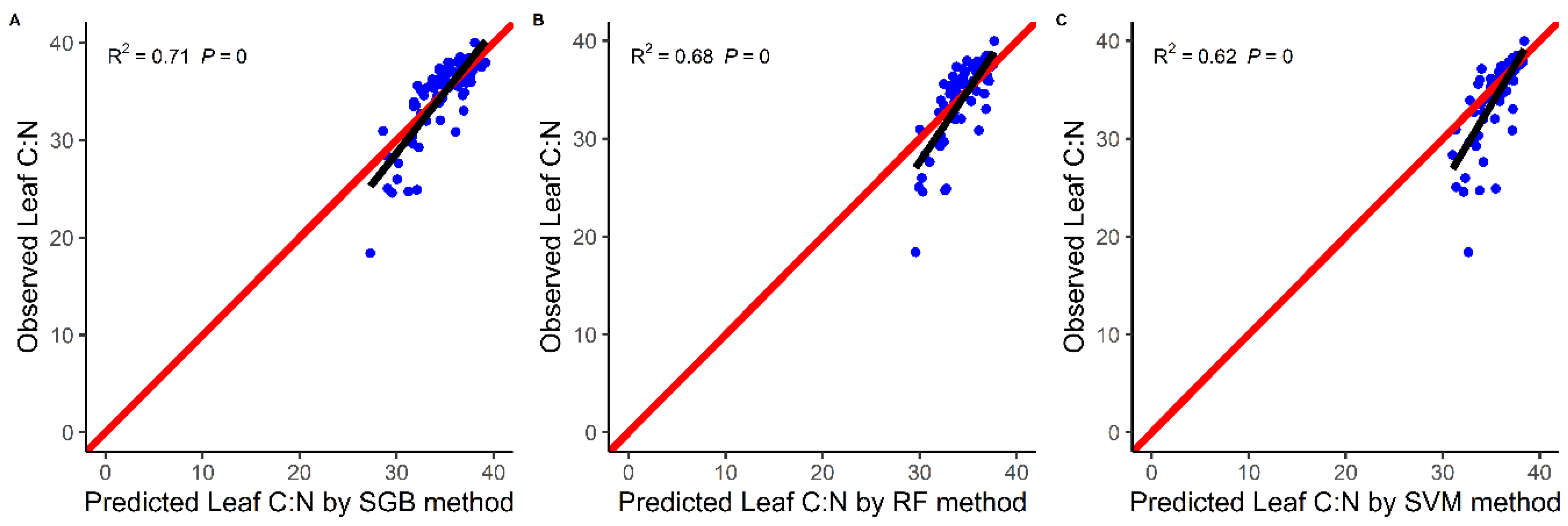
4.1. Models Comparison

The mean MAE, RMSE and R² were varied from 2.06 ± 0.62 to 2.43 ± 0.68, 2.88 ± 0.85 to 24 ± 1.15, and 0.37 ± 0.23 b to 0.51 ± 0.22 a, respectively (Table 2). A significant difference in model fitting parameters was found among different modeling techniques (p < 0.05). However, the post hoc test (LSD) revealed that stochastic gradient boosting (SGB), random forest (RF) and support vector machine (SVM) modeling techniques were not significantly different (p > 0.05;

Table 3. Comparison of model fitting parameters among four modeling methods. Relative improvement of model accuracy, precision and fitness was calculated against partial against partial least squared regression. Columns with the same letter (a or b; group of modeling methods) are not significantly different based on the LSD test (p < 0.05).

Models	Model Accuracy			Relative Improvement			Error Percentage
	MAE	RMSE	R2	MAE%	RMSE%	R2%	MAE%	RMSE%
SGB	2.16 ± 0.58 a	2.88 ± 0.85 a	0.51 ± 0.22 a	−11.11	−11.11	37.84	6.15	8.20
RF	2.21 ± 0.60 a	2.99 ± 1.15 a	0.48 ± 0.24 a	−9.05	−7.72	29.73	6.30	8.52
SVM	2.06 ± 0.62 a	3.12 ± 1.20 a	0.46 ± 0.24 a	−15.23	−3.70	24.32	5.86	8.89
PLSR	2.43 ± 0.68 b	3.24 ± 1.15 b	0.37 ± 0.23 b	0.00	0.00	0.00	6.93	9.23

). However, the model fitting parameters of these three modeling techniques were significantly different from the least performing partial least square regression (PLSR; p < 0.05; Table 3). The relative improvement in terms of MAE, RMSE and R² for the SGB, RF and SVM were estimated against PLSR (the lowest performance model) is shown in Table 2. SGB modeling technique showed best performance in terms of relative improvement of RMSE and R² while SVM showed best performance in of relative improvement of MAE (Table 3). A similar trend in performance to RMSE and R² (relative improvement) was also found for MAE and RMSE percentage of field-based mean C:N (Table 3).

As the three model-evaluating parameters were not varied significantly among SGB, RF and SVM, we also plotted the predicted C:N ratio based on these three models against the field-based C:N ratio for testing its fitness in terms of slope and intercept parameters against the 1:1 line (Figure 2). Observed versus predicted scatter plots showed a strong predictability of the SGB model as the slope was deviated only 0.26 from one, and points were concentrated near the 1:1 line (Figure 2a;

Table 4. Internal validation statistics of observed (field) versus predicted C:N ratio of stochastic gradient boosting (SGB), random forest (RF), and support vector machine (SVM). a: intercept and b: slope.

Model Coefficients	Variables
y = a + b*x	Obs_C:N vs. Pre_CN_SGB	Obs_C:N vs. Pre_CN_RF	Obs_C:N vs. Pre_CN_SVM
a	−9.04	−16.15	−24.38
b	1.26	1.46	1.65
MAE	1.58	1.55	1.51
RMSE	2.12	2.23	2.44
MAE%	4.50	4.41	4.30
RMSE%	6.03	6.34	6.94

). While the SVM had least predictability (Figure 2c; Table 4).

4.2. Importance of Predictors

In different modeling approaches, the importance of the top ten predictors and the type of predictors were different (Figure 3). For instance, in SGB, RF and SVM models top ten predictors were a mixture of different bands, GLCM texture and vegetation indices while in PLSR model top ten predictors consist of GLCM texture of different bands (Figure 3a–d). Moisture and temperature related bands, GLCM texture and vegetation indices were enlisted in the top 10 important predictors in all the models except PLSR where GLCM texture of different bands were in the top ten predictors (Figure 3a–d).

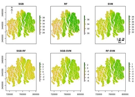
4.3. Spatial and Temporal Distribution of C:N

The spatial distribution of C:N based on the stochastic gradient boosting (SGB), random forest (RF) and support vector machine (SVM) modeling techniques and its prediction difference between the three-modeling techniques is shown in Figure 4. The difference map and statistics of pixel to pixel association of prediction of C:N ratio by different modeling techniques revealed that SGB and RF predictions were slightly different (Figure 4; Table 4). However, a large difference was observed in production of C:N ratio between SGB and SVM and RF and SVM (Table 4; Figure 4). Although, the prediction difference of C:N ratio was quite low between SGB and RF modeling techniques, the SGB modeling technique captured variation of C:N ratio that was closer to field distribution compared to RF (

Table 5. Spatial relationship between different modeling methods in predicting C:N ratio across the whole Sundarbans Reserved Forest. SGB: Stochastic gradient boosting, RF: Random Forest and SVM: Support Vector Machine. a: intercept and b: slope.

Model Coefficients	Variables
y = a + b*x	SGB vs. RF	SGB vs. SVM	RF vs. SVM
a	−3.65	−21.10	−13.86
b	1.10	1.54	1.35
R2	0.92	0.73	0.77
N (pixel)	4499989.00	4499989.00	4499989.00
F (F-test significance)	23,384,941.95	5,155,875.87	6,358,556.93

).

Higher C:N ratio was associated in the eastern part of Sundarbans Reserved Forest with a clear homogenous patch compared to the western part and the landward side of the central part (Figure 4). The streamline zone (near to river and canal bank) had lower C:N ratio compared to stable stands (forest proper zone; 100 to 200 m away from river and canal bank) (Figure 4).

As the SGB modeling technique covered much spatial variation of C:N and were similar to field C:N, we applied the SGB based on Landsat 8 composite image for 2019 to observing the temporal change of C:N (

Table 6. Comparision between spatial statistics (models based) and field C:N ratio. SGB: Stochastic gradient boosting, RF: Random Forest and SVM: Support Vector Machine.

	Mean	Min	Max	SD
Field	35.15	18.4	39.99	3.96
SGB 2010	33.92	26.95	39.43	2.45
RF 2010	34.26	29.36	37.69	2.05
SVM2010	35.68	30.99	38.51	1.16
SGB 2019	32.51	27.04	37.28	1.77

; Figure 5). The difference between 2009–10 and 2019 C:N showed that C:N ratio increased mainly at the central and landward parts of Sundarbans Reserved Forest (Figure 5). In the seaward and eastern side, it showed a decreasing trend in C:N ratio (Figure 5).

5. Discussion

To our current knowledge, this study assessed, for the first time, the spatial distribution and temporal change of the CWM of senescent leaf C:N ratio in Sundarbans Reserved Forest, Bangladesh as a model in mangrove ecosystem with remote sensing. Four machine learning modeling approaches were compared in order to select the best modeling technique for mapping C:N ratio using spectral and textural properties of seven bands and vegetation indices of Landsat TM 5. The modeling approach that combined predictors from the above-mentioned Landsat TM 5 image properties that also related to moisture and temperate, showed better performance compared to the modeling approach that used only textural properties. The SGB modeling technique captured wide variation of C:N ratio and used a lower number of predictors compared to the other three modeling methods. Thus, this modeling technique was applied to the Landsat 8 image in 2019 for assessing temporal change of C:N ratio.

5.1. Comparison of Model Performance

The nonlinear based modeling technique showed better performance in terms of lower MAE, RMSE and higher R² (Table 3). This difference in performance among different modeling approaches could be due to several reasons [47,87]. First, how a specific modeling approach arranges and handles the highly correlated predictors in the top rank of importance and had high correlation with C:N. Although, all the modeling approaches used in this study have the capacity to handle the multicollinearity issue, the SGB showed strong ability to handle multicollinearity over other models [47,87]. In a study of biomass modeling using RapidEye satellite with SGB and RF in Africa terrestrials forest, Dube [50] reported the outperformance of the SGB modeling approach. PLSR showed a weak performance. A similar performance of PLSR modeling technique in comparison with other machine learning modeling approaches has also been reported in biomass modeling studies [88,89,90]. This finding could reveal that C:N ratio and remote sensing-based predictors are nonlinearly related in the Sundarbans Reserved Forest. This could not be handled well by PLSR modeling technique which is linear based [46].

The second reason is the combination of predictors from different dimensions (e.g., either band spectral properties or GLCM textural properties or vegetation indices or all of them) in modeling. The modeling approaches that aggregate both spectral and textural properties have higher predictability compared to the methods that aggregate only a single type of predictor [23,91]. The top three modeling approaches (SGB, RF and SVM) combined the most important predictors from band spectral and GLCM textural properties and vegetation indices compared to PLSR modeling technique, which mainly aggregated the GLCM texture properties of different bands (Figure 3). This incorporation of homogeneous predictors in modeling resulted in the poor performance of PLSR technique.

Finally, the type of predictors in the top rank of important value in different modeling methods are related to vegetation, canopy moisture, salinity and water content. Among the top rank predictors, Band 6 is related to moisture and temperature while the Disease Water Stress Index and Modified Normalized Difference Water Index are related to water stress and canopy moisture, respectively [92,93,94,95]. Previous studies also confirmed that in mangrove, nutrient status and dynamics vary along with water, temperature and salinity gradient [3,7]. Therefore, the modeling technique that had a combination of those predictors in the top rank of importance value had lower errors in prediction and higher capacity of explaining the variance of C:N (Table 2; Figure 3).

5.2. Spatial Distribution and Temporal Change of C:N ratio in SRF

Among the top three modeling approaches, the predicted C:N map stochastic gradient boosting (SGB) technique was closer to the field-based C:N distribution (Figure 4; Table 6). Although, the mean and maximum values of C:N in the predicted map of C:N by the top three models was closer to field value, the SGB technique predicted the lower value of C:N better than RF and SVM (Table 6). The spatial distribution of C:N ratio in Sundarbans Reserved Forest (SRF) was closely related to vegetation types and salinity gradient. For example, the higher C:N value (>36) in the eastern part of SRF is mainly dominated by Heritiera fomes (Figure 4) [16,22,96]. The higher C:N ratio in these areas indicates that Heretiera fomes dominated stand has higher photosynthetic nitrogen use efficiency or nutrient resorption capacity [3,16,97]. However, most of the western parts of SRF were under low C:N ratio coverage, which indicates species in those areas are in stress conditions with low photosynthetic nitrogen use or have lower nutrient resorption capacity and thereby there may be low productivity or carbon sequestration capacity [16]. These areas are mainly dominated by Ceriops decandra and Excoecaria agallocha with scattered Xylocarpus granatum, X. mekongensis [16,96]. A higher level of salinity may cause enzymatic metabolism disorder in the chloroplast; decline in K⁺ ion, the key photosynthetic element and other philological activities, thus decreasing the rate of photosynthesis [97]. For this reason, photosynthetic nitrogen use efficiency could be lower in the high saline zone and streamlined areas in the eastern part of SRF, which could be the cause of low C:N ratio in those zones. The lower range of C:N ratio was also found in the 2010 map in the landward (the northern side of SRF), although this area is associated with freshwater or moderate saline water coverage. The reason of this lower C:N value could be the dominance of Avicenna officinalis species, which has a lower C:N ratio (24.47; Table 1) [13].

The temporal change map (difference between 2009–2010 and 2019) indicates that a gradual increasing trend was observed from seaward to landward (central and western part of SRF; Figure 5). Similar trend also observed at streamline to forest proper line (Figure 5). This could be due to the change of species composition over the 10-years period where species with higher C:N may be shifted. In most cases it was H. fomes because other species (A. corniculatum, R. mucronata) are mainly distributed in high saline area (south-western part of SRF) and some also confined in waterlogged areas (B. sexangular) in SRF. However, temporal change map also shows that across the seaward and eastern part of SRF the C:N ratio was declined (Figure 5). Two reasons may be caused this declination of C:N: (i) a super cyclone (Bulbul) passed over SRF on 9 November 2019 which severely damaged forest canopy and (ii) may be the change of species composition where species with low C:N ratio may come to canopy layer.

5.3. Implication for Forest Health Monitoring and Policy

In the current climate change regime, monitoring of health conditions is a key forest management task [22,33,98]. Litter quality such as C:N ratio as an essential biodiversity variable or functional trait can be used as a potential indicator of decomposition rate, plant nitrogen retention capacity, primary productivity and soil organic carbon storage [6,9,10,99,100].

We developed advance machine learning models for mapping senescence leaf C:N in SRF using Landsat TM 5 imagery and applied the best model on Landsat 8 imagery for 2019. The C:N ratio map developed in the current study can be used for improving the biogeochemical and ecosystem models in the mangroves. In this way, our developed method will contribute to evaluable ecosystem service policy and forest management at the local and regional levels [53,101]. For example, it can be used to track the endangered Red list species in Mangrove that were enlisted by the International Union for Conservation of Nature. The higher value of C:N ratio in the eastern parts of SRF is dominated by H. fomes, the endangered species in SRF. Therefore, by tracking C:N ratio as an indicator of Essential Biodiversity Variable, we can assess the progress of Biodiversity targets that related to IUCN Red List species. For example, two of 20 specific targets (targets 9 and 12) of Aichi Biodiversity Targets-2020 are related to endangered species. The aim of these biodiversity targets is to conserve the threatened species and update their conservation status as to whether they are being improved and sustained by 2020 [102,103]. Furthermore, our developed method directly contributes to monitoring the progress of the biodiversity targets (Aichi Targets 2, 3 and 15), which are related to nutrient dynamic, productivity and ecosystem health [102,104,105]. The C:N ratio is directly associated with key ecosystem functions (decomposition) that have been regarded as biodiversity indicators such as net primary productivity, nutrient retention, disturbance regime [102,104,105], helping in this way to achieve National Biodiversity Target 2 of Bangladesh [106]. While the usage of Landsat imagery in our modeling technique is related to National biodiversity Target 19 of Bangladesh which is aimed at developing a sustainable monitoring technique by means of remote sensing [106]. Ultimately, our finding will be contributed towards achieving sustainable development goal 15 and Aichi Biodiversity target 2, 11 and 15 [51,106,107,108] for Bangladesh.

6. Conclusions

The current study investigated the potentiality of Landsat imagery for spatiotemporal mapping of CWM of C:N ratio of senescent leaf by comparing four machine learning techniques in SRF. SGB technique showed the best performance by incorporating key predictors from the spectral and textural properties and vegetation indices group, which had higher relative improvement against the least performing method (PLSR) compared to RF and SVM. The spatial pattern of C:N ratio map based on SGB method captured a wide variation of C:N, which was closer to field C:N ratio. The map of C:N ratio reveals that the spatial distribution of C:N mainly depends on the species type and salinity gradient. Stands close to the streamline are in a more stressed condition than forest proper or inland side. The eastern side of SRF, which is mostly dominated by H. fomes and receives more freshwater from the upstream river, had a higher C:N ratio, and thereby is in less stressed condition with higher nitrogen use or retention efficiency compared to the western and landward sides of SRF. The temporal change of C:N ratio could also be influenced by species composition change and cyclone damage. Our developed advance machine learning technique thus can be applied for future prediction of litter quality in SRF and for improving the biogeochemical and ecosystem models related to nutrient dynamic in the mangroves.

References

1. Sanderman, J.; Hengl, T.; Fiske, G.; Solvik, K.; Adame, M.F.; Benson, L.; Bukoski, J.J.; Carnell, P.; Cifuentes-Jara, M.; Donato, D.; et al. A global map of mangrove forest soil carbon at 30 m spatial resolution. Environ. Res. Lett. 2018, 13, 55002. [Google Scholar] [CrossRef]
2. Donato, D.C.; Kauffman, J.B.; Murdiyarso, D.; Kurnianto, S.; Stidham, M.; Kanninen, M. Mangroves among the most carbon-rich forests in the tropics. Nat. Geosci. 2011, 4, 293–297. [Google Scholar] [CrossRef]
3. Alongi, D. Impact of Global Change on Nutrient Dynamics in Mangrove Forests. Forests 2018, 9, 596. [Google Scholar] [CrossRef] [Green Version]
4. Alongi, D.M. Carbon sequestration in mangrove forests. Carbon Manag. 2012, 3, 313–322. [Google Scholar] [CrossRef]
5. De Deyn, G.B.; Cornelissen, J.H.C.; Bardgett, R.D. Plant functional traits and soil carbon sequestration in contrasting biomes. Ecol. Lett. 2008, 11, 516–531. [Google Scholar] [CrossRef]
6. Adame, M.F.; Fry, B. Source and stability of soil carbon in mangrove and freshwater wetlands of the Mexican Pacific coast. Wetl. Ecol. Manag. 2016, 24, 129–137. [Google Scholar] [CrossRef] [Green Version]
7. Hossain, M.; Siddique, M.R.H.; Abdullah, S.M.R.; Saha, S.; Ghosh, D.C.; Rahman, M.S.; Limon, S.H. Nutrient Dynamics Associated with Leaching and Microbial Decomposition of Four Abundant Mangrove Species Leaf Litter of the Sundarbans, Bangladesh. Wetlands 2014, 34, 439–448. [Google Scholar] [CrossRef]
8. Kristensen, E.; Bouillon, S.; Dittmar, T.; Marchand, C. Organic carbon dynamics in mangrove ecosystems: A review. Aquat. Bot. 2008, 89, 201–219. [Google Scholar] [CrossRef] [Green Version]
9. Strickland, M.S.; Osburn, E.; Lauber, C.; Fierer, N.; Bradford, M.A. Litter quality is in the eye of the beholder: Initial decomposition rates as a function of inoculum characteristics. Funct. Ecol. 2009, 23, 627–636. [Google Scholar] [CrossRef]
10. Desie, E.; Vancampenhout, K.; Nyssen, B.; van den Berg, L.; Weijters, M.; van Duinen, G.J.; den Ouden, J.; Van Meerbeek, K.; Muys, B. Litter quality and the law of the most limiting: Opportunities for restoring nutrient cycles in acidified forest soils. Sci. Total Environ. 2020, 699, 134383. [Google Scholar] [CrossRef]
11. Chen, R.; Twilley, R.R. Patterns of mangrove forest structure and soil nutrient dynamics along the Shark River Estuary, Florida. Estuaries Coasts 1999, 22, 955–970. [Google Scholar] [CrossRef]
12. Hättenschwiler, S.; Coq, S.; Barantal, S.; Handa, I.T. Leaf traits and decomposition in tropical rainforests: Revisiting some commonly held views and towards a new hypothesis. New Phytol. 2011, 189, 950–965. [Google Scholar] [CrossRef] [PubMed]
13. Chanda, A.; Akhand, A.; Manna, S.; Das, S.; Mukhopadhyay, A.; Das, I.; Hazra, S.; Choudhury, S.B.; Rao, K.H.; Dadhwal, V.K. Mangrove associates versus true mangroves: A comparative analysis of leaf litter decomposition in Sundarban. Wetl. Ecol. Manag. 2016, 24, 293–315. [Google Scholar] [CrossRef]
14. Aber, J.D.; Melillo, J.M.; McClaugherty, C.A. Predicting long-term patterns of mass loss, nitrogen dynamics, and soil organic matter formation from initial fine litter chemistry in temperate forest ecosystems. Can. J. Bot. 1990, 68, 2201–2208. [Google Scholar] [CrossRef] [Green Version]
15. Jacob, M.; Viedenz, K.; Polle, A.; Thomas, F.M. Leaf litter decomposition in temperate deciduous forest stands with a decreasing fraction of beech (Fagus sylvatica). Oecologia 2010, 164, 1083–1094. [Google Scholar] [CrossRef] [PubMed] [Green Version]
16. Mizanur Rahman, M.; Nabiul Islam Khan, M.; Fazlul Hoque, A.K.; Ahmed, I. Carbon stock in the Sundarbans mangrove forest: Spatial variations in vegetation types and salinity zones. Wetl. Ecol. Manag. 2015, 23, 269–283. [Google Scholar] [CrossRef]
17. Wahid, S.M.; Babel, M.S.; Bhuiyan, A.R. Hydrologic monitoring and analysis in the Sundarbans mangrove ecosystem, Bangladesh. J. Hydrol. 2007, 332, 381–395. [Google Scholar] [CrossRef]
18. Iftekhar, M.S.; Saenger, P. Vegetation dynamics in the Bangladesh Sundarbans mangroves: A review of forest inventories. Wetl. Ecol. Manag. 2008, 16, 291–312. [Google Scholar] [CrossRef]
19. Rahman, M.M.; Rahaman, M.M. Impacts of Farakka barrage on hydrological flow of Ganges river and environment in Bangladesh. Sustain. Water Resour. Manag. 2017, 1–14. [Google Scholar] [CrossRef]
20. Richards, D.R.; Friess, D.A. Rates and drivers of mangrove deforestation in Southeast Asia, 2000–2012. Proc. Natl. Acad. Sci. USA 2016, 113, 344–349. [Google Scholar] [CrossRef] [Green Version]
21. Gilman, E.L.; Ellison, J.; Duke, N.C.; Field, C. Threats to mangroves from climate change and adaptation options: A review. Aquat. Bot. 2008, 89, 237–250. [Google Scholar] [CrossRef]
22. Rahman, M.M.; Lagomasino, D.; Lee, S.; Fatoyinbo, T.; Ahmed, I.; Kanzaki, M. Improved assessment of mangrove forests in Sundarbans East Wildlife Sanctuary using WorldView 2 and Tan DEM-X high resolution imagery. Remote Sens. Ecol. Conserv. 2019, 5, 136–149. [Google Scholar] [CrossRef]
23. Moreno-Martínez, Á.; Camps-Valls, G.; Kattge, J.; Robinson, N.; Reichstein, M.; van Bodegom, P.; Kramer, K.; Cornelissen, J.H.C.; Reich, P.; Bahn, M.; et al. A methodology to derive global maps of leaf traits using remote sensing and climate data. Remote Sens. Environ. 2018, 218, 69–88. [Google Scholar] [CrossRef] [Green Version]
24. Díaz, S.; Lavorel, S.; De Bello, F.; Quétier, F.; Grigulis, K.; Robson, T.M. Incorporating plant functional diversity effects in ecosystem service assessments. Proc. Natl. Acad. Sci. USA 2007, 104, 20684–20689. [Google Scholar] [CrossRef] [Green Version]
25. Finegan, B.; Peña-Claros, M.; de Oliveira, A.; Ascarrunz, N.; Bret-Harte, M.S.; Carreño-Rocabado, G.; Casanoves, F.; Díaz, S.; Eguiguren Velepucha, P.; Fernandez, F.; et al. Does functional trait diversity predict above-ground biomass and productivity of tropical forests? Testing three alternative hypotheses. J. Ecol. 2015, 103, 191–201. [Google Scholar] [CrossRef] [Green Version]
26. Tilman, D.; Isbell, F.; Cowles, J.M. Biodiversity and Ecosystem Functioning. Annu. Rev. Ecol. Evol. Syst. 2014, 45, 471–493. [Google Scholar] [CrossRef]
27. Isbell, F.; Craven, D.; Connolly, J.; Loreau, M.; Schmid, B.; Beierkuhnlein, C.; Bezemer, T.M.; Bonin, C.; Bruelheide, H.; de Luca, E.; et al. Biodiversity increases the resistance of ecosystem productivity to climate extremes. Nature 2015, 526, 574–577. [Google Scholar] [CrossRef]
28. Conti, G.; Díaz, S. Plant functional diversity and carbon storage—An empirical test in semi-arid forest ecosystems. J. Ecol. 2013, 101, 18–28. [Google Scholar] [CrossRef]
29. Ali, A.; Yan, E.-R.; Chang, S.X.; Cheng, J.-Y.; Liu, X.-Y. Community-weighted mean of leaf traits and divergence of wood traits predict aboveground biomass in secondary subtropical forests. Sci. Total Environ. 2017, 574, 654–662. [Google Scholar] [CrossRef]
30. Kröber, W.; Li, Y.; Härdtle, W.; Ma, K.; Schmid, B.; Schmidt, K.; Scholten, T.; Seidler, G.; von Oheimb, G.; Welk, E.; et al. Early subtropical forest growth is driven by community mean trait values and functional diversity rather than the abiotic environment. Ecol. Evol. 2015, 5, 3541–3556. [Google Scholar] [CrossRef] [Green Version]
31. Dias, A.T.C.; Berg, M.P.; de Bello, F.; Van Oosten, A.R.; Bílá, K.; Moretti, M. An experimental framework to identify community functional components driving ecosystem processes and services delivery. J. Ecol. 2013, 101, 29–37. [Google Scholar] [CrossRef]
32. Cong, W.-F.; van Ruijven, J.; Mommer, L.; De Deyn, G.B.; Berendse, F.; Hoffland, E. Plant species richness promotes soil carbon and nitrogen stocks in grasslands without legumes. J. Ecol. 2014, 102, 1163–1170. [Google Scholar] [CrossRef]
33. Abelleira Martínez, O.J.; Fremier, A.K.; Günter, S.; Ramos Bendaña, Z.; Vierling, L.; Galbraith, S.M.; Bosque-Pérez, N.A.; Ordoñez, J.C. Scaling up functional traits for ecosystem services with remote sensing: Concepts and methods. Ecol. Evol. 2016, 6, 4359–4371. [Google Scholar] [CrossRef] [PubMed]
34. Wallis, C.I.B.; Homeier, J.; Peña, J.; Brandl, R.; Farwig, N.; Bendix, J. Modeling tropical montane forest biomass, productivity and canopy traits with multispectral remote sensing data. Remote Sens. Environ. 2019, 225, 77–92. [Google Scholar] [CrossRef]
35. Homolová, L.; Malenovský, Z.; Clevers, J.G.P.W.; García-Santos, G.; Schaepman, M.E. Review of optical-based remote sensing for plant trait mapping. Ecol. Complex. 2013, 15, 1–16. [Google Scholar] [CrossRef] [Green Version]
36. Enquist, B.J.; Norberg, J.; Bonser, S.P.; Violle, C.; Webb, C.T.; Henderson, A.; Sloat, L.L.; Savage, V.M. Scaling from Traits to Ecosystems: Developing a General Trait Driver Theory via Integrating Trait-Based and Metabolic Scaling Theories. In Advances in Ecological Research; Academic Press Inc.: Cambridge, MA, USA, 2015; Volume 52, pp. 249–318. [Google Scholar]
37. Chemura, A.; Mutanga, O.; Odindi, J.; Kutywayo, D. Mapping spatial variability of foliar nitrogen in coffee (Coffea arabica L.) plantations with multispectral Sentinel-2 MSI data. ISPRS J. Photogramm. Remote Sens. 2018, 138, 1–11. [Google Scholar] [CrossRef]
38. Gara, T.W.; Darvishzadeh, R.; Skidmore, A.K.; Wang, T.; Heurich, M. Accurate modelling of canopy traits from seasonal Sentinel-2 imagery based on the vertical distribution of leaf traits. ISPRS J. Photogramm. Remote Sens. 2019, 157, 108–123. [Google Scholar] [CrossRef]
39. Ollinger, S.V.; Richardson, A.D.; Martin, M.E.; Hollinger, D.Y.; Frolking, S.E.; Reich, P.B.; Plourde, L.C.; Katul, G.G.; Munger, J.W.; Oren, R.; et al. Canopy nitrogen, carbon assimilation, and albedo in temperate and boreal forests: Functional relations and potential climate feedbacks. Proc. Natl. Acad. Sci. USA 2008, 105, 19336–19341. [Google Scholar] [CrossRef] [Green Version]
40. Woitchik, A.F.; Ohowa, B.; Kazungu, J.M.; Rao, R.G.; Goeyens, L.; Dehairs, F. Nitrogen Enrichment during Decomposition of Mangrove Leaf Litter in an East African Coastal Lagoon (Kenya): Relative Importance of Biological Nitrogen Fixation; Kluwer Academic Publishers: Berlin, Germany, 1997; Volume 39. [Google Scholar]
41. Nordhaus, I.; Salewski, T.; Jennerjahn, T.C. Food preferences of mangrove crabs related to leaf nitrogen compounds in the Segara Anakan Lagoon, Java, Indonesia. J. Sea Res. 2011, 65, 414–426. [Google Scholar] [CrossRef]
42. Fonte, S.J.; Schowalter, T.D. Decomposition of Greenfall vs. Senescent Foliage in a Tropical Forest Ecosystem in Puerto Rico1. Biotropica 2004, 36, 474. [Google Scholar] [CrossRef]
43. Zarco-Tejada, P.J.; Ustin, S.L. Modeling canopy water content for carbon estimates from MODIS data at land EOS validation sites. IGARSS 2001 Scanning the Present and Resolving the Future. In Proceedings of the IEEE 2001 International Geoscience and Remote Sensing Symposium 2001, Trento, Italy, 13–14 September 2001; Volume 1, pp. 342–344, (Cat. No.01CH37217). [Google Scholar]
44. Clevers, J.G.P.W.; Kooistra, L.; Schaepman, M.E. Using spectral information from the NIR water absorption features for the retrieval of canopy water content. Int. J. Appl. Earth Obs. Geoinf. 2008, 10, 388–397. [Google Scholar] [CrossRef]
45. Omer, G.; Mutanga, O.; Abdel-Rahman, E.M.; Peerbhay, K.; Adam, E. Mapping leaf nitrogen and carbon concentrations of intact and fragmented indigenous forest ecosystems using empirical modeling techniques and WorldView-2 data. ISPRS J. Photogramm. Remote Sens. 2017, 131, 26–39. [Google Scholar] [CrossRef]
46. Sun, X.; Li, G.; Wang, M.; Fan, Z. Analyzing the uncertainty of estimating forest aboveground biomass using optical imagery and spaceborne LiDAR. Remote Sens. 2019, 11, 722. [Google Scholar] [CrossRef] [Green Version]
47. De’Ath, G.; Fabricius, K.E. Classification and regression trees: A powerful yet simple technique for ecological data analysis. Ecology 2000, 81, 3178–3192. [Google Scholar] [CrossRef]
48. Lawrence, R.; Bunn, A.; Powell, S.; Zambon, M. Classification of remotely sensed imagery using stochastic gradient boosting as a refinement of classification tree analysis. Remote Sens. Environ. 2004, 90, 331–336. [Google Scholar] [CrossRef]
49. Elith, J.; Leathwick, J.R.; Hastie, T. A working guide to boosted regression trees. J. Anim. Ecol. 2008, 77, 802–813. [Google Scholar] [CrossRef]
50. Dube, T.; Mutanga, O.; Elhadi, A.; Ismail, R. Intra-and-Inter Species Biomass Prediction in a Plantation Forest: Testing the Utility of High Spatial Resolution Spaceborne Multispectral RapidEye Sensor and Advanced Machine Learning Algorithms. Sensors 2014, 14, 15348–15370. [Google Scholar] [CrossRef] [Green Version]
51. Convention on Biological Diversity (CBD). The Strategic Plan for Biodiversity 2011–2020 and the Aichi Biodiversity Targets; CBD: New York, NY, USA; Rio de Janeiro, Brazil, 2011. [Google Scholar]
52. Convention on Biological Diversity. National Targets. Available online: https://www.cbd.int/countries/targets/?country=bd (accessed on 20 December 2019).
53. MOEF. Integrated Resources Management Plans for the Sundarbans; Ministry of Environment and Forests: Dhaka, Bangladesh, 2010; Volume 1, ISBN 978-3-902762-17-7.
54. Rahman, M.S.; Hossain, G.M.; Khan, S.A.; Uddin, S.N. An annotated checklist of the vascular plants of Sundarban Mangrove Forest of Bangladesh. Bangladesh J. Plant. Taxon. 2015, 22, 17–41. [Google Scholar] [CrossRef] [Green Version]
55. Islam, S.; Feroz, S.M.; Ahmed, Z.U.; Chowdhury, H.; Khan, R.I.; Al-Mamun, A. Species richness and diversity of the floristic composition of the Sundarbans mangrove reserve forest, Bangladesh in relation to spatial habitats and salinity. Malayian For. 2016, 79, 7–38. [Google Scholar]
56. Hamilton, S.E.; Casey, D. Creation of a high spatio-temporal resolution global database of continuous mangrove forest cover for the 21st century (CGMFC-21): CGMFC-21. Glob. Ecol. Biogeogr. 2016, 25, 729–738. [Google Scholar] [CrossRef]
57. Forest Department-Government of the People\’s Republic of Bangladesh. Available online: http://www.bforest.gov.bd/site/page/f619019f-14cd-481a-86f4-1d5b4ae40515/- (accessed on 23 April 2020).
58. Aziz, A.; Paul, A. Bangladesh Sundarbans: Present Status of the Environment and Biota. Diversity 2015, 7, 242–269. [Google Scholar] [CrossRef]
59. Uddin, M.S.; de Ruyter van Steveninck, E.; Stuip, M.; Shah, M.A.R. Economic valuation of provisioning and cultural services of a protected mangrove ecosystem: A case study on Sundarbans Reserve Forest, Bangladesh. Ecosyst. Serv. 2013, 5, 88–93. [Google Scholar] [CrossRef]
60. Laliberté, E.; Legendre, P. A distance-based framework for measuring functional diversity from multiple traits. Ecology 2010, 91, 299–305. [Google Scholar] [CrossRef] [PubMed]
61. Mensah, S.; Veldtman, R.; Assogbadjo, A.E.; Glèlè Kakaï, R.; Seifert, T. Tree species diversity promotes aboveground carbon storage through functional diversity and functional dominance. Ecol. Evol. 2016, 6, 7546–7557. [Google Scholar] [CrossRef] [PubMed]
62. Garnier, E.; Cortez, J.; Billès, G.; Navas, M.L.; Roumet, C.; Debussche, M.; Laurent, G.; Blanchard, A.; Aubry, D.; Bellmann, A.; et al. Plant functional markers capture ecosystem properties during secondary succession. Ecology 2004, 85, 2630–2637. [Google Scholar] [CrossRef]
63. Flood, N. Seasonal composite landsat TM/ETM+ Images using the medoid (a multi-dimensional median). Remote Sens. 2013, 5, 6481–6500. [Google Scholar] [CrossRef] [Green Version]
64. The Thematic Mapper Landsat Science. Available online: https://landsat.gsfc.nasa.gov/the-thematic-mapper/ (accessed on 5 March 2020).
65. Haralick, R.M.; Dinstein, I.; Shanmugam, K. Textural Features for Image Classification. IEEE Trans. Syst. Man Cybern. 1973, SMC-3, 610–621. [Google Scholar] [CrossRef] [Green Version]
66. Conners, R.W.; Trivedi, M.M.; Harlow, C.A. Segmentation of a high-resolution urban scene using texture operators (Sunnyvale, California). Comput. Vis. Graph. Image Process. 1984, 25, 273–310. [Google Scholar] [CrossRef]
67. Bello, C.; Galetti, M.; Pizo, M.A.; Magnago, L.F.S.; Rocha, M.F.; Lima, R.A.F.; Peres, C.A.; Ovaskainen, O.; Jordano, P. Defaunation affects carbon storage in tropical forests. Sci. Adv. 2015, 1, 1–11. [Google Scholar] [CrossRef] [Green Version]
68. Blackburn, G.A. Spectral indices for estimating photosynthetic pigment concentrations: A test using senescent tree leaves. Int. J. Remote Sens. 1998, 19, 657–675. [Google Scholar] [CrossRef]
69. Rama Rao, N.; Garg, P.K.; Ghosh, S.K.; Dadhwal, V.K. Estimation of leaf total chlorophyll and nitrogen concentrations using hyperspectral satellite imagery. J. Agric. Sci. 2008, 146, 65–75. [Google Scholar] [CrossRef]
70. Volesky, J.C.; Stern, R.J.; Johnson, P.R. Geological control of massive sulfide mineralization in the Neoproterozoic Wadi Bidah shear zone, southwestern Saudi Arabia, inferences from orbital remote sensing and field studies. Precambrian Res. 2003, 123, 235–247. [Google Scholar] [CrossRef]
71. Apan, A.; Held, A.; Scientific, T.C.; Phinn, S. Formulation and Assessment of Narrow-Band Vegetation Indices from EO-1 Hyperion Imagery for Detecting Sugarcane Disease; Spatial Sciences: Adelaide, Australia, 2003. [Google Scholar]
72. Los, S.O.; Collatz, G.J.; Bounoua, L.; Sellers, P.J.; Tucker, C.J.; Los, S.O.; Collatz, G.J.; Bounoua, L.; Sellers, P.J.; Tucker, C.J. Global Interannual Variations in Sea Surface Temperature and Land Surface Vegetation, Air Temperature, and Precipitation. J. Clim. 2001, 14, 1535–1549. [Google Scholar] [CrossRef]
73. Hewson, R.D.; Cudahy, T.J.; Huntington, J.F. Geologic and alteration mapping at Mt fitton, South Australia, using ASTER satellite-borne data. In Proceedings of the International Geoscience and Remote Sensing Symposium (IGARSS), Trento, Italy, 13–14 September 2001; Volume 2, pp. 724–726. [Google Scholar]
74. Fensholt, R.; Sandholt, I. Derivation of a shortwave infrared water stress index from MODIS near- and shortwave infrared data in a semiarid environment. Remote Sens. Environ. 2003, 87, 111–121. [Google Scholar] [CrossRef]
75. Xu, H. Modification of normalised difference water index (NDWI) to enhance open water features in remotely sensed imagery. Int. J. Remote Sens. 2006, 27, 3025–3033. [Google Scholar] [CrossRef]
76. Al-Khaier, F. Soil Salinity Detection Using Satellite Remotes Sensing; International Institute for Geo-Information Science and Earth Observation: Enschede, The Netherlands, 2003. [Google Scholar]
77. Ridgeway, G. Generalized Boosted Models: A guide to the gbm package. Compute 2007, 1, 1–12. [Google Scholar]
78. Friedman, J.H. Stochastic gradient boosting. Comput. Stat. Data Anal. 2002, 38, 367–378. [Google Scholar] [CrossRef]
79. Breiman, L. Random Forests. Mach. Learn. 2001, 45, 5–32. [Google Scholar] [CrossRef] [Green Version]
80. Liaw, A.; Wiener, M. Classification and Regression by Random Forest. R News 2002, 2, 18–22. [Google Scholar]
81. Vapnik, V.N. Statistical Learning Theory; Wiley: Hoboken, NJ, USA, 1998; ISBN 9780471030034. [Google Scholar]
82. Karatzoglou, A.; Meyer, D.; Hornik, K. Support Vector Algorithm in R. J. Stat. Softw. 2006, 15, 1–28. [Google Scholar] [CrossRef] [Green Version]
83. Smola, A.J.; Schölkopf, B. A tutorial on support vector regression. Stat. Comput. 2004, 14, 199–222. [Google Scholar] [CrossRef] [Green Version]
84. Peng, J.; Ji, W.; Ma, Z.; Li, S.; Chen, S.; Zhou, L.; Shi, Z. Predicting total dissolved salts and soluble ion concentrations in agricultural soils using portable visible near-infrared and mid-infrared spectrometers. Biosyst. Eng. 2016, 152, 94–103. [Google Scholar] [CrossRef]
85. Ali, A.M.; Skidmore, A.K.; Darvishzadeh, R.; van Duren, I.; Holzwarth, S.; Mueller, J. Retrieval of forest leaf functional traits from HySpex imagery using radiative transfer models and continuous wavelet analysis. ISPRS J. Photogramm. Remote Sens. 2016, 122, 68–80. [Google Scholar] [CrossRef] [Green Version]
86. RStudio Team. RStudio: Integrated Development for R; RStudio Inc.: Boston, MA, USA, 2019. [Google Scholar]
87. Cutler, D.R.; Edwards, T.C.; Beard, K.H.; Cutler, A.; Hess, K.T.; Gibson, J.; Lawler, J.J. Random Forests for Classification in Ecology. Ecology 2007, 88, 2783–2792. [Google Scholar] [CrossRef] [PubMed]
88. Breunig, F.M.; Galvão, L.S.; Dalagnol, R.; Dauve, C.E.; Parraga, A.; Santi, A.L.; Della Flora, D.P.; Chen, S. Delineation of management zones in agricultural fields using cover–crop biomass estimates from PlanetScope data. Int. J. Appl. Earth Obs. Geoinf. 2020, 85, 102004. [Google Scholar] [CrossRef]
89. Zhang, Y.; Liang, S.; Sun, G. Forest biomass mapping of northeastern china using GLAS and MODIS data. IEEE J. Sel. Top. Appl. Earth Obs. Remote Sens. 2014, 7, 140–152. [Google Scholar] [CrossRef]
90. Shen, W.; Li, M.; Huang, C.; Tao, X.; Wei, A. Annual forest aboveground biomass changes mapped using ICESat/GLAS measurements, historical inventory data, and time-series optical and radar imagery for Guangdong province, China. Agric. For. Meteorol. 2018, 259, 23–28. [Google Scholar] [CrossRef] [Green Version]
91. Cao, L.; Pan, J.; Li, R.; Li, J.; Li, Z. Integrating airborne LiDAR and optical data to estimate forest aboveground biomass in arid and semi-arid regions of China. Remote Sens. 2018, 10, 532. [Google Scholar] [CrossRef] [Green Version]
92. Houborg, R.; Fisher, J.B.; Skidmore, A.K. Advances in remote sensing of vegetation function and traits. Int. J. Appl. Earth Obs. Geoinf. 2015, 43, 1–6. [Google Scholar] [CrossRef] [Green Version]
93. Croft, H.; Arabian, J.; Chen, J.M.; Shang, J.; Liu, J. Mapping within-field leaf chlorophyll content in agricultural crops for nitrogen management using Landsat-8 imagery. Precis. Agric. 2019, 1–25. [Google Scholar] [CrossRef] [Green Version]
94. Anderson, M.C.; Neale, C.M.U.; Li, F.; Norman, J.M.; Kustas, W.P.; Jayanthi, H.; Chavez, J. Upscaling ground observations of vegetation water content, canopy height, and leaf area index during SMEX02 using aircraft and Landsat imagery. Remote Sens. Environ. 2004, 92, 447–464. [Google Scholar] [CrossRef]
95. Questad, E.J.; Kellner, J.R.; Kinney, K.; Cordell, S.; Asner, G.P.; Thaxton, J.; Diep, J.; Uowolo, A.; Brooks, S.; Inman-Narahari, N.; et al. Mapping habitat suitability for at-risk plant species and its implications for restoration and reintroduction. Ecol. Appl. 2014, 24, 385–395. [Google Scholar] [CrossRef] [PubMed]
96. Rahman, M.M.; Kabir, M.E.; Ahmed, I. Protected Areas for Climate Change Mitigation and Livelihood Option: A Case Study of the Bangladesh Sundarbans Mangrove Forest; Springer: Tokyo, Japan, 2017; pp. 119–136. [Google Scholar]
97. Ball, M.C. Ecophysiology of mangroves. Trees 1988, 2, 129–142. [Google Scholar] [CrossRef]
98. Kissling, W.D.; Ahumada, J.A.; Bowser, A.; Fernandez, M.; Fernández, N.; García, E.A.; Guralnick, R.P.; Isaac, N.J.B.; Kelling, S.; Los, W.; et al. Building essential biodiversity variables (EBVs) of species distribution and abundance at a global scale. Biol. Rev. 2018, 93, 600–625. [Google Scholar] [CrossRef] [PubMed] [Green Version]
99. Bakker, M.A.; Carreño-Rocabado, G.; Poorter, L. Leaf economics traits predict litter decomposition of tropical plants and differ among land use types. Funct. Ecol. 2011, 25, 473–483. [Google Scholar] [CrossRef]
100. Gessner, M.O.; Swan, C.M.; Dang, C.K.; McKie, B.G.; Bardgett, R.D.; Wall, D.H.; Hättenschwiler, S. Diversity meets decomposition. Trends Ecol. Evol. 2010, 25, 372–380. [Google Scholar] [CrossRef]
101. McCall, M.K.; Chutz, N.; Skutsch, M. Moving from Measuring, Reporting, Verification (MRV) of Forest Carbon to Community Mapping, Measuring, Monitoring (MMM): Perspectives from Mexico. PLoS ONE 2016, 11, e0146038. [Google Scholar] [CrossRef]
102. O’Connor, B.; Secades, C.; Penner, J.; Sonnenschein, R.; Skidmore, A.; Burgess, N.D.; Hutton, J.M. Earth observation as a tool for tracking progress towards the Aichi Biodiversity Targets. Remote Sens. Ecol. Conserv. 2015, 1, 19–28. [Google Scholar] [CrossRef]
103. Petrou, Z.I.; Manakos, I.; Stathaki, T. Remote sensing for biodiversity monitoring: A review of methods for biodiversity indicator extraction and assessment of progress towards international targets. Biodivers. Conserv. 2015, 24, 2333–2363. [Google Scholar] [CrossRef]
104. Branquinho, C.; Serrano, H.C.; Nunes, A.; Pinho, P.; Matos, P. Essential Biodiversity Change Indicators for Evaluating the Effects of Anthropocene in Ecosystems at a Global Scale; Springer: Cham, Switzerland, 2019; pp. 137–163. [Google Scholar]
105. Vihervaara, P.; Auvinen, A.P.; Mononen, L.; Törmä, M.; Ahlroth, P.; Anttila, S.; Böttcher, K.; Forsius, M.; Heino, J.; Heliölä, J.; et al. How Essential Biodiversity Variables and remote sensing can help national biodiversity monitoring. Glob. Ecol. Conserv. 2017, 10, 43–59. [Google Scholar] [CrossRef]
106. Latest NBSAPs. Available online: https://www.cbd.int/nbsap/about/latest/#bd (accessed on 20 December 2019).
107. Strategic Plan for Biodiversity 2011–2020, Including Aichi Biodiversity Targets. Available online: https://www.cbd.int/sp/ (accessed on 20 December 2019).
108. Unit, B. Strategic Plan for Biodiversity 2011–2020, Including Aichi Biodiversity Targets; CBD: New York, NY, USA; Rio de Janeiro, Brazil, 2019. [Google Scholar]
Figure 1. Distribution of sampling plots in Sundarbans Reserved Forest.
Remotesensing 12 01375 g001
Figure 2. Scatter plot of observed leaf carbon to nitrogen (C:N) ratio versus predicted leaf C:N by of stochastic gradient boosting (a), random forest (b) and support vector machine (c) methods. The bold point (blue) indicates the value of C:N in each plot. Red and black lines indicate the 1:1 reference line and best fit linear, respectively.
Remotesensing 12 01375 g002
Figure 3. Importance value of predictors in each of the four modeling techniques based on 10-fold cross-validation with 10 times repetition. The codes after band (e.g., B6_savg) and other predictors were explained in Table 2. (a) Stochastic gradient booting; (b) random forest; (c) support vector machine; (d) partial least square regression.
Remotesensing 12 01375 g003
Figure 4. Spatial distribution (upper row) and differrence (lower row) of C:N ratio bewteen models across the whole Sundarbans Reserved Forest for 2009–2010. SGB: Stochastic gradient boosting, RF: Random Forest and SVM: Support Vector Machine.
Remotesensing 12 01375 g004
Figure 5. Spatial (upper row) and temporal change (lower row) map of C:N ratio based on stochastic gradient boosting modeling method from 2010 to 2019. SGB: Stochastic gradient boosting, RF: Random Forest and SVM: Support Vector Machine.
Remotesensing 12 01375 g005