Radar Interferometry: 20 Years of Development in Time Series Techniques and Future Perspectives

Abstract

The research and improvement of methods to be used for deformation measurements from space is a challenge. From the previous 20 years, time series Synthetic Aperture Radar (SAR) interferometry techniques have proved for their ability to provide millimeter-scale deformation measurements over time. This paper aims to provide a review of such techniques developed in the last twenty years. We first recall the background of interferometric SAR (InSAR). We then provide an overview of the InSAR time series methods developed in the literature, describing their principles and advancements. Finally, we highlight challenges and future perspectives of the InSAR in the Big Data era.

1. Introduction

Interferometric Synthetic Aperture Radar (InSAR) time series techniques are powerful geodetic remote sensing approaches for estimating millimetric surface deformation from space. The interferometric phase, which is associated with the optical path between the SAR’s sensor and the sensed area, can be obtained by taking advantage of the geometry between two SAR acquisitions [1]. However, this technique presents issues relating to signal decorrelations (e.g., spatial/temporal decorrelations [2], and atmospheric disturbances [1,3], that cannot be efficiently compensated), which limit the reliable deformation of the ground from the entire interferograms [1]. InSAR time series analysis techniques focus on tackling the signal decorrelations to estimate the deformation and atmospheric signal. We can divide these techniques into three groups. The first approach is Permanent/Persistent Scatterer (PS) techniques, which analyze the time-coherent point scatterers mainly available in urban areas [4,5,6]. The second approach consists of Distributed Scatterer (DS) targets, which have relaxed the restriction on the phase stability and expanded areas that are affected by signal decorrelations thanks to the redundant network of interferograms [7,8]. The final approach relates to hybrid methods, which analyze the time series phase change of both PS and DS targets [9,10].

The Copernicus Earth observation program headed by the European Commission in partnership with the European Space Agency (ESA) led to the launching of the Sentinel-1 mission [11]. ESA’s Sentinel-1 mission allows a systematic global mapping of the Earth’s surface based on Terrain Observation by Progressive Scans technique [12]. This leads to an unprecedented time series dataset of InSAR. This is also true for the next Tandem-L [13] and NISAR missions [14]. The challenge is to extend time series InSAR analysis to exploit Big InSAR Data such as to large coverages, mapping countries, and continents for long term monitoring.

This paper aims to provide an overview of 20 years of methodology advancement in InSAR time series techniques for measuring surface deformation from space. This review is organized as follows: the mathematical model background is provided in Section 2; the main PS algorithm is examined in Section 3; the DS technique is discussed in Section 4; the combination of PS and DS techniques is reported in Section 5; and finally the challenges and the associated future research are discussed in Section 6.

2. Background

Let us suppose that N SAR images are available for a certain area of interest. The images are co-registered on a reference grid and phase contributions due to terrain topography and orbit have been compensated. The residual phase of the unwrapped differential interferogram ${\phi }^n$ is composed of the phase contributions related to residual topography, deformation, atmosphere, and noise [1]:

$${\phi }^n={\phi }_{topo}^n+{\phi }_{defo}^n+{\phi }_{aps}^n+{\phi }_{noise}^n+2k\pi$$

(1)

where ${\phi }_{topo}^n$ is the residual topographic phase; ${\phi }_{defo}^n$ is the deformation phase; ${\phi }_{aps}^n$ is the atmospheric phase screen, which represents the signal delay due to weather conditions; k is an integer ambiguity number; and ${\phi }_{noise}^n$ is the phase noise due to temporal decorrelation, mis-coregistration, uncompensated spectral shift decorrelation, orbital errors, soil moisture, and thermal noise.

The residual topographic phase for a point p is given as follows [1]:

$${\phi }_{p,topo}^n=k_p^z{\epsilon }_p^z$$

(2)

where $k_p^z=\frac{4\pi b_n}{\lambda sin\theta R_n}$ is the height-to-phase factor, ${\epsilon }_p^z$ is the elevation error; $b_n$ is the normal baseline relative to the n-th image with respect to the reference (master) image; $\theta$ is the local incidence angle; $\lambda$ is the carrier wavelength; $R_n$ is the (zero-Doppler) distance between the target and the n-th orbit acquisition.

The phase component due to the displacement at the point p can be usefully split into two components:

$${\phi }_{p,defo}^n=k^t{v}_p+{\mu }_{NL}$$

(3)

where v is the constant velocity (light of sight); $k^t=\frac{4\pi t_n}{\lambda }$ is the time-to-phase factor; $t_n$ is the temporal baseline; and ${\mu }_{NL}$ is the phase term due to a possible non-linear motion.

The atmospheric phase screen ${\phi }_{aps}^n$ is not modeled, but it can be reduced significantly by considering the phase differences of two points nearby. The noise term ${\phi }_{noise}^n$ contains all other phase contributions.

Normally a linear model for the elevation error and the constant velocity is assumed. In detail, given $N-1$ unwrapped differential interferograms, for each pixel, from Equation (1), we can write a linear system of $N-1$ equations and two unknowns:

$${\phi }^n=k^z{\epsilon }^z+k^{t}v+w^n+2k\pi$$

(4)

where $w^n={\mu }_{NL}+{\phi }_{aps}^n+{\phi }_{noise}^n$ is the residual phase. If the integer ambiguity number k is known, the problem of Equation (4) will be linear. Unfortunately, the biggest challenge in the radar interferometry is that the ${\phi }^n$ can be only observed as a wrapped phase (i.e., k is an unknown as well) [1,15]. PS and PSDS analyses can be carried out from the wrapped phase, whereas the unwrapped phase is required in small baseline approaches. Within the last 20 years, the development of the InSAR time series can be summarized in

Table 1. Characteristics of the main Interferometric Synthetic Aperture Radar (InSAR) time series approaches.

Method Reference	Interferogram Network	Pixel Selection Criteria	Deformation Model and Others
Persistent Scattering Interferometry
Ferretti et al. (2000, 2001) [4,5]	Single master	Amplitude dispersion	Linear deformation
Werner et al. (2003) [16]	Single master	Amplitude dispersion and spectral phase diversity	Linear deformation
Hooper et al. (2004) [6]	Single master	Phase stability	Spatial smoothness and 3D phase unwrapping
Kampes (2006) [17]	Single master	Amplitude dispersion	Different types of deformation models
Perissin and Wang (2012) [18]	Target-dependent subset	Quasi-PS approach	Linear deformation
Devanthéry et al. (2014) [19]	Small baseline	Amplitude dispersion and Cousin PS	Spatial smoothness
Siddique et al. (2016) [20]	Single master	Amplitude dispersion and spectral diversity	Different types of deformation models and tomography
Small baseline
Berardino et al. (2002) [7]	Small baseline	Coherence	Spatial smoothness
Mora et al. (2003) [21]	Small baseline	Coherence	Linear deformation
Schmidt and Bürgmann (2003) [22]	Small baseline	Coherence	Spatial and temporal smoothness
Lanari et al. (2004) [8]	Small baseline	Coherence	Spatial smoothness and full-resolution
Crosetto et al. (2005) [23]	Small baseline	Coherence	Stepwise linear function
López-Quiroz et al. (2009) [24]	Small baseline	Coherence	Spatial smoothness
Hetland et al. (2012) [25]	Small baseline	Coherence	Different types of deformation models
Casu et al. (2014) [26] and Manuta et al. (2019) [27]	Small baseline	Coherence	Spatial smoothness and parallel
The combination of PS and DS
Hooper et al. (2008) [9]	Single master and small baseline	Phase stability	Spatial smoothness and 3D phase unwrapping
Ferretti et al. (2011) [10]	Full stacking	Statistical homogeneity test	Linear deformation and phase linking
Goel and Adam (2014) [28]	Small baseline	Statistical homogeneity test	Linear deformation
Samiei-Esfahany et al. (2016) [29]	Full stacking	Statistical homogeneity test	Different types of deformation and phase linking
Cao et al. (2016) [30], Engelbrecht and Inggs (2016) [31]	Full stacking	Statistical homogeneity test	Linear deformation, phase linking, and multiple scattering
Ansari et al. (2017) [32]	Efficient stacking	Statistical homogeneity test	Linear deformation and phase linking
Mullissa et al. (2018) [33]	Full stacking	Statistical homogeneity test	Linear deformation, phase linking, and polarization

.

3. Persistent Scattering Interferometry

Developed in the late 1990s, the Permanent Scatters interferometry is the first operational InSAR technique for time series analysis [4,5]. From the measured wrapped phase in Equation (4), the estimation of parameters is possible only if the signal-to-noise ratio (SNR) is high enough. Consequently, instead of working on the entire image, the analysis is based only on a subset of image pixels which is characterized by highly coherent targets (i.e., low ${\sigma }_{noise}^2$). Such a stable target is named Permanent Scatter (PS) [4], which is characterized by a dominant scatterer within resolution elements. The selection of PS is based on criteria from the amplitude-based time series.

Let us now consider the phase difference between two neighboring PS (e.g., target p and q) which can be written as [4]:

$$\Delta {\phi }_{pq}^n=W\left\{k_p^z\Delta {\epsilon }_{pq}^z+k^t\Delta v_{pq}+\Delta w_{pq}^n\right\}$$

(5)

where W is the wrapping operator; $\Delta {\epsilon }_{pq}^z$ is the relative elevation error; $\Delta v_{pq}$ is the relative constant velocity; and $\Delta w_{pq}^n={\mu }_{pq,NL}^n+{\phi }_{pq,aps}^n+{\phi }_{pq,noise}^n$ is the phase difference between the model and measurement between points p and q in the n-th interferogram.

The residue phase variance ${\sigma }_{\Delta w}^2$ is the sum of three contributions ${\sigma }_{\mu }^2$, ${\sigma }_{aps}^2$, and ${\sigma }_{noise}^2$ because they are independent random variables. Since we consider a pair of neighboring PS not too far apart, it implies low ${\sigma }_{aps}^2$, i.e., less than 0.1 $ra{d}^2$ for low distance 1 km [4]. Further, if the motion of a neighboring targets is correlated, ${\sigma }_{\mu }^2$ should be low. Consequently, ${\sigma }_{\Delta w}^2$ is low as expected at the PS pixels. It is then possible to estimate $\Delta {\epsilon }^z$ and $\Delta v$ with a high degree of accuracy. Two parameters are determined as the values of $\Delta {\epsilon }^z$ and $\Delta v$ that maximize the complex ensemble coherence in time ${\widehat{\gamma }}_{pq}$ defined as [4]:

$${\widehat{\gamma }}_{pq}=\frac{1}{N-1}\sum _{n=1}^{N-1}exp\left(i▵w_{pq}^n\right)$$

(6)

under the condition:

$$\Delta w_{pq}^n\le \pi .$$

(7)

The coherence absolute varies from 0 to 1, where a coherence value of 1 means a complete fit of the observed and the modeled phase. If the ensemble coherence of a PS pair is lower than a given threshold (i.e., 0.75), it will then discarded in the processing.

In this way, $▵w_{pq}^n$ as well as $\Delta {\epsilon }_{pq}^z$ and $\Delta v_{pq}$ can be computed for every PS pair. However, the largest distance of a PS pair should be kept shorter than the typical atmospheric decorrelation length (i.e., less than 1 km) in order to guarantee the condition of Equation (7). Whenever the estimations of $\Delta {\epsilon }^z$ and $\Delta v$ have been done, our interest parameters ${\epsilon }^z$ and v can be calculated by integrating their relative values ($\Delta {\epsilon }^z$ and $\Delta v$) from pairs of neighboring pixels with respect to a reference pixel (i.e., the motion and elevation are known). In other words, we can recover the unwrapped phase difference $\Delta {\phi }^n$ and integrate them over the whole network of PS pixels.

Now since the $▵w_p^n$ at the point p is recovered as the unwrapped residual phase, it is possible to separate the atmospheric component by applying spatial-temporal filtering. After the atmospheric delays are calculated at the PS targets, it can be interpolated at the entire interferograms, so-called “atmospheric phase screen” (APS).

The success of this PS method is strongly dependent on the density of the selected PS. By subtracting the interpolated APSs from the differential interferograms, it is possible to add PS points (i.e., based on phase rather than amplitude stability), resulting in a more dense set of PSs. After all, the same computations as described in the previous are repeated.

However, this PS technique is likely to fail in areas where the initial PS selection (i.e., based on amplitude stability), does not suffice to interpolate APSs. Particularly, it is evident in the case of nature and non-urban areas. The first attempt to this problem was proposed by Hooper et al. [6], who selected the point based on the stability of the phase. The selected points are called Persistent Scatterers. This phase-based algorithm has been reported to yield a more dense point on nature areas (e.g., rock and volcano) than the amplitude-based method. Finally, since the Permanent Scatters method is protected by a patent [5], we use the term Persistent Scatterer Interferometry (PSI) to refer to techniques that exploit InSAR time series at individual scatterers.

The Related PSI Techniques and Advancements

The innovation introduced by PSI is not only in the selection of stable targets but also on their use to remove the atmospheric phase screen artifacts. The PSI technique demonstrated that using a time series SAR images is a way to obtain accurate estimates despite temporal and geometrical decorrelation. This leads to the development of many related techniques in the literature by using a modified approach, e.g., Interferometric Point Target Analysis [16], Coherent Target Monitoring [34], Stanford Method for Persistent Scatters (StaMPS) [6], Spatial Temporal Unwrapping Network (STUN) [17], Persistent Scatterer Pairs [35], Quasi Persistent Scatterers [18], and Cousin PS [19]. These approaches seek to improve the PSI technique using a modified pixel selection criteria and different types of deformation models. The most different approach refers to STUN, where the author proposed an integer least-squares estimator to solve Equation (5) without considering the condition described in Equation (7). In addition to amplitude-based algorithms, many methods are proposed to add more reliable PS candidates, e.g., spectral phase diversity [16], phase stability criterion [6], and maximum likelihood [36], resulting in a denser point for reliable phase estimations. The linear deformation model can be extended to monitor seasonal motion phenomena [37] or to consider thermal expansion [38].

One of the most widely used PSI methods is StaMPS given by Hooper et al. [6]. The advantage of this approach relies on a phase-based PS selection, no assumption on a prior deformation model in the processing, and a three-dimensional phase unwrapping approach. This work is originated from the same name PSI software packages, StaMPS [9,39].

The signal model in Equation (1) assumes that there is one dominant scatterer within the resolution cell. In practice, there could be more than one dominant point. For example, it is the case of a layover due to tower buildings. To relax this assumption, SAR tomography, which can resolve layovers based on multi-baseline InSAR [40], can be used. In Siddique et al. [20], the authors demonstrated that the SAR tomography method can add the improved value in deformation sampling in areas affected by layover. In addition, by the virtue of SAR tomography, the scatterer’s elevation and intensity are considered in the analysis, solving a question posed by Jia and Liu [41].

The PSI requires a long time series, leading to an averaging effect. For example, if stable points are decorrelated in the majority of the low-coherence interferograms, their identifications may be discarded [42]. This leads to lower significantly the overall SNR, resulting in a loss of information. To address this, the PS assumption is relaxed by considering targets that are visible in a subset of the data set, e.g., temporary-PS [42,43] and quasi-PS [18]. Finally, Ferretti et al. [10] proposed a Maximum Likelihood framework to consider slowly decorrelating targets within the PSI processing, which we will discuss in detail in Section 5.

4. Small Baseline

Many studies have been investigated to perform InSAR time series over areas where the assumption of PS may not be retained, i.e., Distributed Scatterers (DS) which are usually corresponding to debris, desert, and non-cultivated land areas. Many works are based on minimizing target decorrelation effects by the exploitation of the redundant network of interferograms (i.e., a subset of interferograms with the shortest temporal and/or spatial baselines possible) [7,8,44]. Comparing to the PSI technique, they include many DS scatterers, that may be decorrelated in longer baseline combinations [2].

4.1. The SBAS Inversion

The Small Baseline Subset (SBAS) approaches account for signal decorrelations by partitioning the data set into several subsets with short spatial and temporal baseline possible (i.e., excluded large baseline interferograms) [7]. Within the subsets, the interferograms are spatially multilooked and unwrapped. For example, the integer ambiguity number k is estimated so that the model in Equation (4) is linear now.

Let us suppose that M unwrapped differential interferograms are available by generating from N SAR images. The stack of unwrapped interferograms M is co-registered on a reference grid and phase terms due to terrain topography and orbit have been compensated. The SBAS analysis can be considered as a linear model inversion problem. For each pixel, based on Equation (4), the functional model is described as [7]:

$$\phi =Ax+\Delta w$$

(8)

where A is a $M(N-1)$ design matrix indicating the small baseline interferogram generations. For example, for each row, it consists of −1, 0, and 1, in which −1 is for the reference image, 1 represents secondary acquisition, and 0 is for the rest. x is the vector of the unknowns (${\epsilon }^z$ and v). $\Delta w$ is the interferometric phase residual that includes the non-linear motion, atmosphere, noises, and phase-unwrapping errors. Comparing to the PSI, the unwrapping error is introduced in SBAS because the unwrapped interferogram can be biased (i.e., by adding a wrong integer ambiguity number ($2\pi$) during the phase unwrapping [15]).

If the design matrix A is full rank (i.e., fully connected network), x can be estimated by an unbiased weighted least-squares. If the network is non-fully connected, the estimation of x can be carried out by a singular value decomposition (SVD) [7,22].

The inverted performance can be assessed by using temporal-based coherence ${\gamma }_{temp}$ defined as [45]:

$${\gamma }_{temp}=\frac{1}{M}exp\left(j(\phi -A\widehat{\phi })\right)$$

(9)

It is worth to note that the temporal coherence ${\gamma }_{temp}$ accounts for phase-unwrapping errors by definition, resulting in a more reliable indicator than spatial-based coherence [46]. Similar to the PSI technique, the SBAS selects good candidates which are highly coherent. In practice, a threshold for the temporal coherence ${\gamma }_{temp}$ (i.e., 0.75) can be used to select reliable pixels.

4.2. Overview Advancements

Since the work of Berardino et al. [7] was proposed, many modified SBAS techniques were investigated in the literature, e.g., New SBAS [47], Small Temporal Baseline Subset (STBAS) [48], Multiscale InSAR Time-Series [25], Miami INsar Timeseries software in PYthon (MintPy) [46]. The original SBAS is based on multilook imagery and maybe not suitable for studying at local-scale deformations [7]. This drawback was improved by extending the SBAS method for full-resolution (i.e., single look) data [8]. Temporal decorrelations can be minimized by using short temporal baselines [2]. Based on this, only interferograms with short temporal baselines are used and demonstrated in STBAS [48]. Many methods are different from the selection of initial pixels which can be based on the calculation of coherent, e.g., all interferograms [7,25,49], a minimum number for every acquisition [46], and a total minimum number [47]. Recently, a parallel SBAS algorithm (P-SBAS) has been proposed for massive amounts of InSAR data [26,27].

To separate the atmospheric phase screen, similar to PSI, the SBAS method relies on the spatio-temporal filtering of the InSAR time-series phase [7,21]. However, it is not as robust as PSI due to the contribution of unwrapping errors. The atmospheric delay is one of the most difficult signals to model because it includes systematic biases and stochastic components [1,50]. Many works have been investigated to mitigate the atmospheric artifacts in order to correct interferograms by using: (1) empirical relationship between topography and tropospheric delay [51,52]; and (2) external data such as numerical weather models [51,53,54,55], MERIS/MODIS [56], and GPS/GNSS observations [55,57]. Recently, Generic Atmospheric Correction Online Service (GACOS) represents the state-of-the-art product, i.e., zenith delay maps, for correcting interferograms [55,58].

To correct the unwrapping errors, both the space and time domain can be used. With the space-based domain, unwrapping errors add phase offsets in a reliable region [15,59]. For a given neighboring reliable region pair, if we assume its phase difference is less than $\pi$, then the unwrapping error can be corrected by adding the integer $2\pi$ phase offsets to each reliable region [46]. With the time-based domain, unwrapping errors can break the consistency of interferogram triplets (i.e., the phases of a loop of the interferograms of three images I${}_1$-I${}_2$, I${}_2$-I${}_3$, I${}_3$-I${}_1$, that would be zero for any point scatterer) [60,61]. Several works have been pursued by using the closure phase of interferogram triplets information. In Biggs et al. [60], the unwrapping errors are visually identified and corrected by adding the $2\pi$ phase offsets to the wrong regions. In Hussain et al. [62], the phase closure of interferogram triplets is used to adjust the network cost during unwrapping.

If the interferogram network is disconnected (i.e., no overlap in spatial/temporal baseline), the SBAS inversion can be strongly biased [8,24,63]. In general, the more the network redundancy improves the network inversion, the more precise estimation can be achieved for the time series phases [46]. For new generation SAR satellites (i.e., Sentinel-1), the fully connected interferograms network can be easily guaranteed to have an unbiased inversion [27,63].

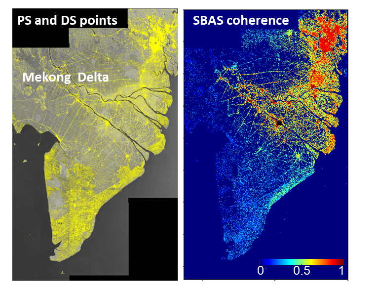
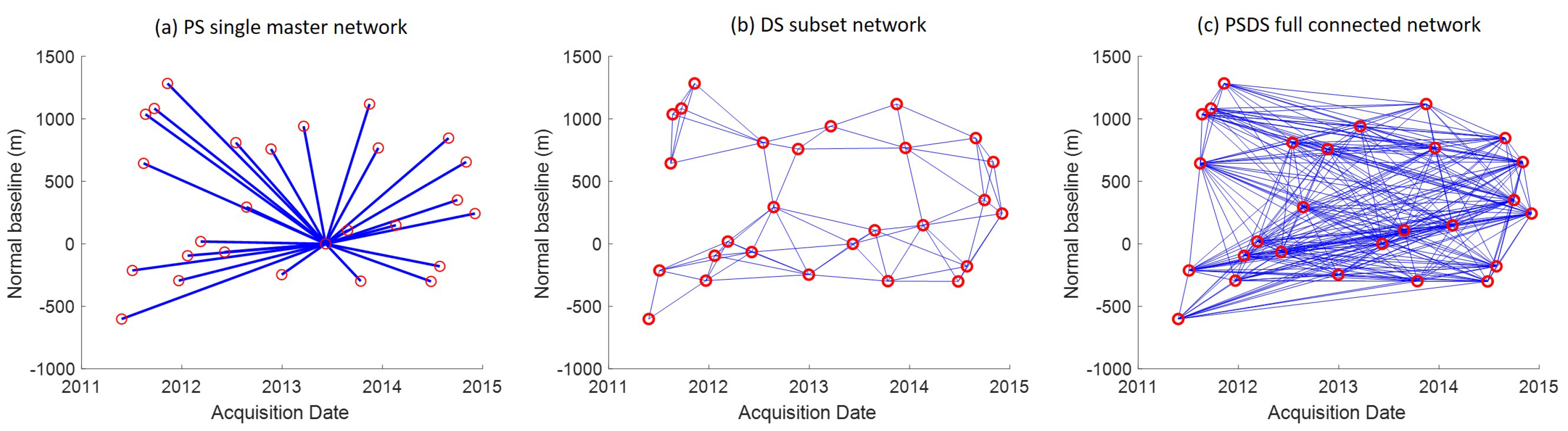
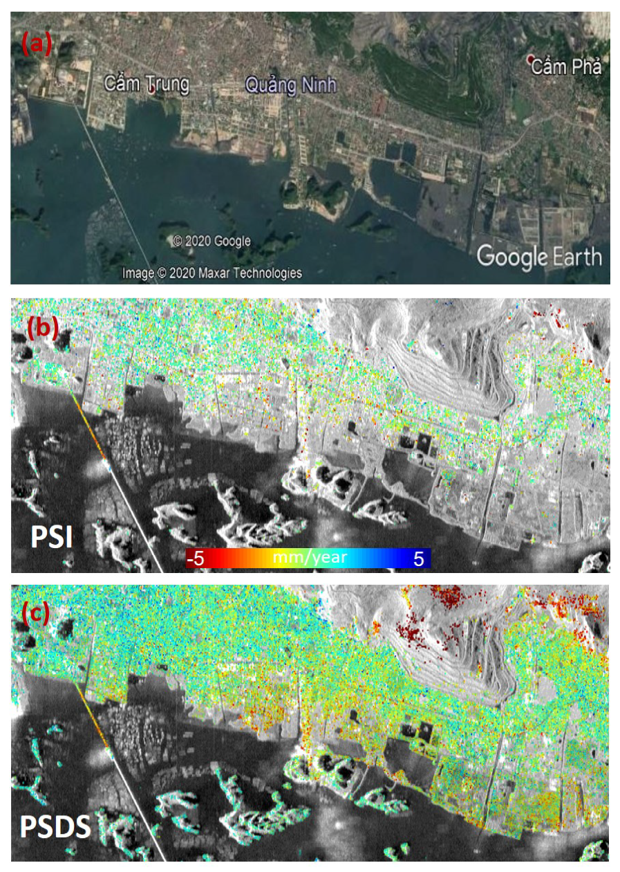
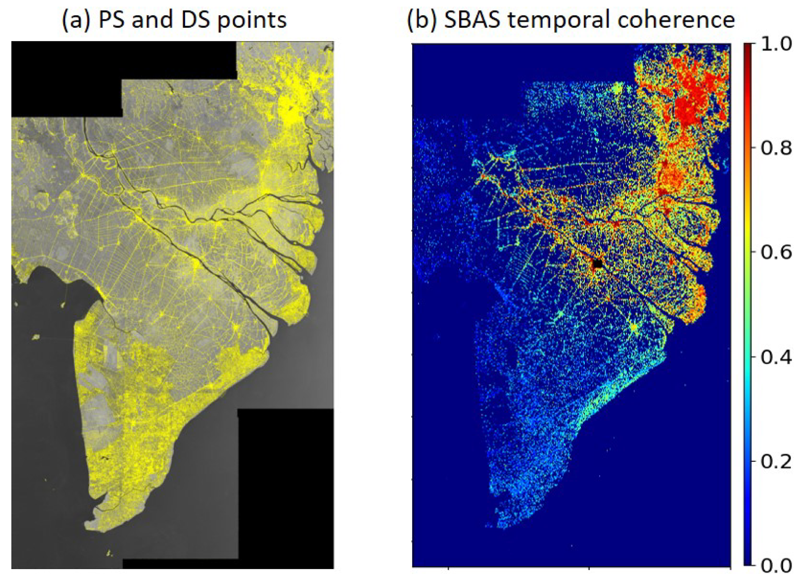
5. The Combination of PS and DS

The motivation for combining PS and DS is to reduce the sparsity of the grid for identified measurement points and to maximize the amount of information available from interferograms. This combination has been investigated by many authors [9,10,64,65,66]. In [9], Hooper proposed a hybrid processing chain where two algorithms (PS and SBAS) are applied, and then SBAS results are inverted by an SVD to combine with PS. On the contrary, in [10,64,65,66], the combination of PS and DS was investigated by Maximum Likelihood (ML) estimation frameworks. The motivation of ML estimations is to use target statistics (i.e., ensemble coherences) to extract the parameters of interest by maximizing a statistical estimator. By this design, coherences are used to directly derive the weight of each interferogram during the estimation process, through a mathematical approach [64]. In addition, due to the properties of the ML, the parameters estimates are asymptotically unbiased and of minimum variance. However, the main limitation of the ML approaches is the need for reliable target statistics (i.e., coherence estimates are not biased). In [65], the authors proposed the ML estimation for both the elevation error and the constant velocity directly from the data. Although this estimator is the most robust, due to the model estimation carried out in a single step, this involves an overwhelming computational load.

5.1. The PSDS Technique

Thanks to the work of [10,66], the ML estimation process can be divided into two steps. First, the ML estimation is applied, in which all the $N(N-1)/2$ interferograms available from N images are jointly exploited to squeeze the best estimates $N-1$ interferometric phases, so-called “SqueeSAR”. This step is known as Phase Linking (PL) [67] or Phase Triangulation Algorithm (PTA) [10] and the estimation of $N-1$ phase series from all possible $N(N-1)/2$ interferograms is referred to as PL. Although the PL computational load is very low, the same performance as the one-step ML estimation can be approximated (as long as the $N(N-1)/2$ interferometric phases have been estimated with sufficient accuracy). Once the estimate of the $N-1$ linked phases has been produced, the second step is necessary to remove the signal decorrelations and estimate the parameters of interest (e.g., the elevation error and the constant velocity), as in PSI processing algorithm. Since the SqueeSAR is protected by a patent [10], the term PSDS refers nowadays to techniques that exploit the time series phase change of both PS and DS targets. In Figure 1, an example of the exploitation of interferogram networks in the InSAR time series techniques is provided. The figure was generated by using Cosmos SkyMed data over Ha Noi area [68].

It is worth to note that PSI can be derived as a special case of ML interferometry, where each PS target is equally correlated in all the images. This is why we do not need to process jointly all the $N(N-1)$ interferograms in the PS, but just to remove the master phase from all the others to get the $N-1$ linked phases. Therefore, the PSDS algorithm is an extension of the PSI algorithm.

DS Selection

The main difficulty of dealing with the DS target is that its average temporal coherence is typically low, due to both geometrical and temporal decorrelation phenomena [2], resulting in low signal-to-noise ratio. However, if the number of pixels sharing the same statistically homogeneous behavior is high enough, it is possible to enhance its signal-to-noise ratio and then to become PS.

To select DS candidates, pixels within a neighborhood that behave similarly are identified. Such pixels are referred to as statistically homogeneous pixels (SHPs). They can be identified by applying a two-sample Kolmogorov–Smirnov test (with a certain level of significance) on the amplitude-based time series of the current pixel and all neighbors contained within a window around it. Pixels with a similar cumulative probability distribution (CDF) become “brother”, whereas adjacent pixels with different CDF are discarded. In this way, a brotherhood is created, resulting in a family of SHPs. The DS candidate is identified as having a number of SHP greater than a certain threshold. We then can compute its sample coherence matrix by taking advantage of its SHP family. The coherence matrix ($\widehat{\mathsf{\Gamma }}$) can fully characterize the target statistics and is used to invert for $N-1$ linked phase ($\widehat{\mathit{\lambda }}$) as [10]:

$$\widehat{\mathit{\lambda }}=argma{x}_{\lambda }\left\{{\Lambda }^H\left(|\widehat{\mathsf{\Gamma }}{|}^{-1}\circ \widehat{\mathsf{\Gamma }}\right)\Lambda \right\}$$

(10)

where $\Lambda =exp\left(j\mathit{\lambda }\right)$; ${}^H$ indicates Hermitian conjugation; and ∘ represents the Hadamard entry-wise product. To optimize the phase values, a quasi-Newton method for unconstrained non-linear optimization, i.e., Broyden–Fletcher–Goldfarb–Shanno algorithm [69], can be used. After this procedure, the DS phase values are actually filtered, resulting in more reliable phase unwrapping. The quality of the estimated $N-1$ phase values $\widehat{\lambda }$ can be assessed using the PTA coherence defined as [10]:

$${\gamma }_{PTA}=\frac{2}{N(N-1)}Re\sum _{n=1}^N\sum _{k=n+1}^{N}exp\left(i({\varphi }^{nk}-{\vartheta }^n+{\vartheta }^k)\right)$$

(11)

where ${\varphi }^{nk}$ is the phase corresponding in off-diagonal elements of the coherence matrix $\widehat{\mathsf{\Gamma }}$; and ${\vartheta }^n$ is the estimated phase (the element of $\widehat{\mathit{\lambda }}$).

If the ${\gamma }_{PTA}$ coherence is above a certain threshold, a DS point with the linked $N-1$ phase value will replace the original points. Finally, the selected DS will jointly process with the PS using the same PSI technique (see Section 3).

An example of the velocity map estimated by PSI and PSDS techniques is shown in Figure 2. The figure was generated by using 117 Sentinel-1 images (2015–2019) processed by TomoSAR [70]. A comparison of the measuring point density can be drawn between 126,500 PSDS and 29,500 PS points identified within an area of about 40 km${}^2$.

5.2. Overview Advancements

Decorrelating targets poses a challenge to time series InSAR techniques. To overcome this challenge, the ML estimation was proposed to retrieve the linked phase time-series [66,67], leading to commonly use the PSDS technique as a replacement of PSI due to its remarkable out-performance particularly in nonurban areas [10]. Consequently, this approach becomes the main technique for surface deformation applications [28,30,68,71,72]. Many works have been dedicated to improving the estimation of the linked phase time series and the selection of SHPs.

Regarding the selection of SHPs, many modified approaches, e.g., Anderson–Darling test [28], time-series likelihood ratios [73], t-test [74], fast statistically homogeneous pixel selection [75], mean amplitude difference [76], and similar time-series interferometric phase [77], are proposed to increase the DS points, resulting in the bias mitigation of the sample coherence. The conventional DS assumes independent small scatterers with a uniform scattering mechanism. This assumption can be relaxed by considering the DS targets dominated by two or more scattering mechanisms [30,31]. In Engelbrecht et al. [31], the authors demonstrated that the adding value of the multiple scattering mechanisms approaches in L-band ALOS PalSAR enhances the ability to extract deformation measurements in dynamic agricultural regions. Recently, an attempt has shown that the adding value of polarimetric information can lead to the increase of the number of coherent pixels by a factor of eight with respect to a single-polarization channel [33].

Regarding the estimation of the linked phase, since this is the key step in the PSDS technique, dedicated researches focus on improving its estimation and computational efficiency. In Cao et al. [78], the authors introduced equal-weighted and coherence-weighted factors in phase estimation. Samiei-Esfahany et al. [29] extended the PSI STUN algorithm [17], i.e., based on the integer least-squares principle, to account for decorrelating targets. For the multiple scattering mechanisms, a specific Component extrAction and sElection SAR (CAESAR) algorithm [79], can be applied to extract different scattering components from the coherence matrix [30]. Finally, Ansari et al. [32,80] proposed a recursive estimation (Sequential Estimator) of the sample coherence matrix and an eigen decomposition-based ML estimator which represent one of the best processing schemes, particularly matching for the analysis of the Big InSAR Data.

6. Looking forward in Big InSAR Data Era

From the previous 20 years, time series InSAR analysis has proved to be a precise tool for monitoring the deformation of the Earth’s surface. Most of the works are based on the exploitation of PS [5] and DS [7]. PSs are deterministic targets that often correspond to man-made objects widely available over an urban but are less present in non-urban areas. To overcome this problem, many works exploit DSs to minimize the effect of signal decorrelations through the exploitation of a subset of interferograms. The combination of PS and DS has been considered through the ML estimation [10,28,71] or non-ML framework [29,79]. Compared to the previous algorithms (e.g., based solely on PS and DS), the increased density of PS and DS measurement points provides increased confidence in estimations from the PSDS algorithm. Thus, the PSDS becomes the main tool of time series InSAR analysis due to its remarkable effect, particularly in nonurban areas.

First, thanks to the systematic survey of the globe from current SAR missions, there are many examples demonstrate how the availability of Big Data hints new results. In Xu and Sandwell [81], the authors were able to remove the effect of the earth tides, improving the quality of the long term interferometry, especially in L-band. Another example is provided by Ansari et al. in [82] where a systematic bias (i.e., apparent motion of 0.03 rad/day) appears in long sequences of interferometric data taken on DS targets. It disappears on the PS, obviously, but also on the DS, provided that the coherence should be considered at a rather long (i.e., more than one month) time distance. There is no explanation for this bias unless a possible hypothesis is due to vegetation growth. A third case is the effect of soil moisture on DSs and the break the consistency of interferogram triplets, as studied in [61,83,84]. In fact, in the case of soil penetration and the presence of volume effects, the change of moisture entails a progressive change of the travel time with the penetration depth and thus in a behavior that is inconsistent with any point scatterer. This behavior has been related successfully to the soil moisture retrieved content. Finally, the availability of Big Data is pushing ahead new methodologies based on Artificial Intelligence. Indeed, coherent change detection is possible to make the systems “intelligent” by introducing an additional feature to be evaluated [85]. It is probably too soon to be able to identify real successes in this domain, but the researchers should be alerted to these possibilities.

Second, current SAR missions are delivering an unprecedented InSAR dataset. Although they offer the best opportunity for deformation monitoring, it is a challenge for time series InSAR analysis due to a massive volume for processing. In fact, this challenge is one of the big questions early raised by Crosetto et al. [86]. Recently, there are two initiative processing schemes, e.g., P-SBAS for DS [26,27] and Sequential Estimator for PSDS [32], which can be represented a generic guideline to tackle processing in massive amounts of data.

To make a better understanding of the future picture, we provide an example of the random access memory (RAM) requirement over the low Mekong Delta area in Vietnam. To cover Mekong Delta-wide, a full resolution Sentinel-1 image, characterized by 3 swaths and 10 bursts (i.e., 25,200 pixels in azimuth and 67,500 pixels in range direction, covering about 300 km × 250 km), is stored in complex values with about 14 GB memory data. From 2015–2019, 55 Sentinel-1 images were selected to test the performance, resulting in 750 GB. The information only at the PSDS measure points (i.e., 14 $\times {10}^6$) was extracted, whereas in the SBAS processing, multilook (i.e., 3 in azimuth and 15 in range direction, resulting in 38 $\times {10}^6$ pixels) was applied to increase SNR, see in Figure 3. For the SBAS approach, MintPy was used [46], whereas the PSDS analysis was carried out by TomoSAR [70]. We assume the same requirement of memory (i.e., four times) to process signals in both PSDS and SBAS methods. With PSDS, it requires 24 GB RAM to process, whereas the SBAS method needs 67 GB (i.e., 4 × 750/45 GB). Hence, with the capacity of RAM of 128/256 GB (in 2020), it is possible to handle such 55 images amounts of data. However, the problem is that it is available more than 250 Sentinel-1 images now (February 2020) and there is much more in the near future. Is there a possibility to solve this problem? With the SBAS analysis, the best solution is to reduce the number of images to meet the memory requirement. With the PSDS processing, it needs future works, e.g., maturity of the Sequential Estimator [32] or simplification InSAR products [87], to develop novel methods to process such Big InSAR Data.

Finally, the slow development of new satellites, an endeavor that takes many years, allows having a glimpse of the possible evolution of the SAR systems, enabling the continuity of the Big Data. For now, it can be summarized as follows.

• High Resolution Wide Swath (HRWS) systems [88,89], i.e., a typically 5 m resolution, are coupled with a 12 days revisit time and on a 250 km swath width. This would imply a 4 times improvement on Sentinel-1, and it could be a possibility for the Copernicus Next Generation systems. To achieve that new systems, i.e., Scan-on-Receive, should be used to exploit a taller antenna and hence improve its resolution.
• Satellite constellations (e.g., Capella (www.capellaspace.com), ICEYE (www.iceye.com), Umbra (www.umbralab.com), and XpressSAR (www.xpresssar.com)) are proposed. Indeed, mini-satellites are being used to achieve, in X-band, a meter scale resolution on a limited number of images per day. Then, the possible high number of satellites and their agility would lead to enticing extremely short times to achieve a high-resolution image and always shorter than one day revisit.
• Many satellite systems have been identified and assessed [89,90]. These satellite formations consist of many mini-satellites combined in a multiple-transmit multiple-receive (MIMO) or a single-transmit multiple-receive (SIMO) structure. They can achieve results similar to the principle of HRWS, but maybe with more robust and flexible systems. It should be observed, though, that the formations are difficult to localize their obits precisely, and therefore it would not be possible to guarantee their performances, unless on a statistical basis. Furthermore, many baselines would be available at the same time due to the presence of many satellites, e.g., 4 or 5, and hence up to 10 different baselines. This would allow doing tomography without effects of temporal decorrelation [91] and thus could be used for foliage penetration and forest studies [92,93].
• GEO-synchronous systems are proposed in various modes [94]. The first case is an L-band system [95], i.e., a wide antenna (about 25 m diameter), proposed by Chinese scientists and it is soon be launched. The second case is a smaller C-band system (about 7.5 m antenna diameter). This is being studied within the framework of the ESA Earth Explorer 10-th round, i.e., G-Class [96], and might be the system selected in future decisions to be taken in 2020/2021. The smaller antenna of the European proposal implies a longer observation time in order to achieve good noise performances. However, both systems allow daily observations (and in the European case, hourly) on the part of the globe fronting the satellite. In other words, the fast availability of new images, in the cases of need, will be obtained. The objective is to study the soil moisture and the temporal evolution of columnar water vapor (on a km scale and in time of minutes), that was said to be a disturbance for InSAR processing, but it is going now to be the signal to be studied.

To conclude, the InSAR time series is a powerful technique able to measure millimetric surface deformation from space. SAR missions, e.g., Sentinel-1, NISAR, and future satellites, offer an unprecedented InSAR dataset. Thus, new efficient concepts and methods for InSAR data processing are essential in order to meet the challenge of the Big Data era, enabling operational projects such as national or supranational initiatives for long term deformation monitoring.

References

1. Hanssen, R.F. Radar Interferometry: Data Interpretation and Error Analysis; Kluwer Academic Publishers: Dordrecht, The Netherlands, 2001. [Google Scholar]
2. Zebker, H.A.; Villasenor, J. Decorrelation in interferometric radar echoes. IEEE Trans. Geosci. Remote Sens. 1992, 30, 950–959. [Google Scholar] [CrossRef] [Green Version]
3. Zebker, H.A.; Rosen, P.A.; Hensley, S. Atmospheric effects in interferometric synthetic aperture radar surface deformation and topographic maps. J. Geophys. Res. Solid Earth. 1997, 102, 7547–7563. [Google Scholar] [CrossRef]
4. Ferreti, A.; Prati, C.; Rocca, F. Nonlinear subsidence rate estimation using permanent scatterers in differential SAR interferometry. IEEE Trans. Geosci. Remote Sens. 2000, 38, 2202–2212. [Google Scholar] [CrossRef] [Green Version]
5. Ferretti, A.; Prati, C.; Rocca, F. Permanent scatterers in SAR interferometry. IEEE Trans. Geosci. Remote Sens. 2001, 39, 8–20. [Google Scholar] [CrossRef]
6. Hooper, A.; Zebker, H.; Segall, P.; Kampes, B. A new method for measuring deformation on volcanoes and other natural terrains using InSAR persistent scatterers. Geophys. Res. Lett. 2004, 31, L23661. [Google Scholar] [CrossRef]
7. Berardino, P.; Fornaro, G.; Lanari, R.; Sansosti, E. A New Algorithm for Surface Deformation Monitoring Based on Small Baseline Differential SAR Interferograms. IEEE Trans. Geosci. Remote Sens. 2002, 40, 2375–2383. [Google Scholar] [CrossRef] [Green Version]
8. Lanari, R.; Mora, O.; Manunta, M.; Mallorqui, J.J.; Berardino, P.; Sansosti, E. A small-baseline approach for investigating deformations on full-resolution differential SAR interferograms. IEEE Trans. Geosci. Remote Sens. 2004, 42, 1377–1386. [Google Scholar] [CrossRef]
9. Hooper, A. A multi-temporal InSAR method incorporating both persistent scatterer and small baseline approaches. Geophys. Res. Lett. 2008, 35, 1–5. [Google Scholar] [CrossRef] [Green Version]
10. Ferretti, A.; Fumagalli, A.; Novali, F.; Prati, C.; Rocca, F.; Rucci, A. A New Algorithm for Processing Interferometric Data-Stacks: SqueeSAR. IEEE Trans. Geosci. Remote Sens. 2011, 49, 3460–3470. [Google Scholar] [CrossRef]
11. Torres, R.; Snoeij, P.; Geudtner, D.; Bibby, D.; Davidson, M.; Attema, E.; Rommena, B.; Flourya, N.; Brown, M.; Travera, I.G.; et al. GMES Sentinel-1 mission. Remote Sens. Environ. 2012, 120, 9–24. [Google Scholar] [CrossRef]
12. De Zan, F.; Monti Guarnieri, A. TOPSAR: Terrain Observation by Progressive Scans. IEEE Trans. Geosci. Remote Sens. 2006, 44, 2352–2360. [Google Scholar] [CrossRef]
13. Hajnsek, I.; Shimada, M.; Eineder, M.; Papathanassiou, K.; Motohka, T.; Watanabe, M.; Ohki, M.; De Zan, F.; Lopez-Dekker, P.; Krieger, G.; et al. Tandem-L: Science Requirements and Mission Concept. In Proceedings of the EUSAR 2014; 10th European Conference on Synthetic Aperture Radar, Berlin, Germany, 3–5 June 2014; pp. 1–4. [Google Scholar]
14. Rosen, P.A.; Kim, Y.; Kumar, R.; Misra, T.; Bhan, R.; Sagi, V.R. Global persistent SAR sampling with the NASA-ISRO SAR (NISAR) mission. In Proceedings of the 2017 IEEE Radar Conference (RadarConf), Seattle, WA, USA, 8–12 May 2017; pp. 0410–0414. [Google Scholar]
15. Ghiglia, D.C.; Pritt, M.D. Two-Dimensional Phase Unwrapping: Theory, Algorithms, and Software; John Wiley & Sons, Inc.: New York, NY, USA, 1998. [Google Scholar]
16. Werner, C.; Wegmuller, U.; Strozzi, T.; Wiesmann, A. Interferometric point target analysis for deformation mapping. In Proceedings of the 2003 IEEE International Geoscience and Remote Sensing Symposium, Toulouse, France, 21–25 July 2003; Volume 7, pp. 4362–4364. [Google Scholar] [CrossRef]
17. Kampes, B. Radar Interferometry: Persistent Scatterer Technique; Springer Publishing Company: Dordrecht, The Netherlands, 2006. [Google Scholar]
18. Perissin, D.; Wang, T. Repeat-Pass SAR Interferometry With Partially Coherent Targets. IEEE Trans. Geosci. Remote Sens. 2012, 50, 271–280. [Google Scholar] [CrossRef]
19. Devanthéry, N.; Crosetto, M.; Monserrat, O.; Cuevas-González, M.; Crippa, B. An Approach to Persistent Scatterer Interferometry. Remote Sens. 2014, 6, 6662–6679. [Google Scholar] [CrossRef] [Green Version]
20. Siddique, M.A.; Wegmüller, U.; Hajnsek, I.; Frey, O. Single-Look SAR Tomography as an Add-On to PSI for Improved Deformation Analysis in Urban Areas. IEEE Trans. Geosci. Remote Sens. 2016, 54, 6119–6137. [Google Scholar] [CrossRef]
21. Mora, O.; Mallorqui, J.J.; Broquetas, A. Linear and nonlinear terrain deformation maps from a reduced set of interferometric SAR images. IEEE Trans. Geosci. Remote Sens. 2003, 41, 2243–2253. [Google Scholar] [CrossRef]
22. Schmidt, D.A.; Bürgmann, R. Time-dependent land uplift and subsidence in the Santa Clara valley, California, from a large interferometric synthetic aperture radar data set. J. Geophys. Res. Solid Earth 2003, 108. [Google Scholar] [CrossRef] [Green Version]
23. Crosetto, M.; Crippa, B.; Biescas, E. Early detection and in-depth analysis of deformation phenomena by radar interferometry. Eng. Geol. 2005, 79, 81–91. [Google Scholar] [CrossRef]
24. López-Quiroz, P.; Doin, M.P.; Tupin, F.; Briole, P.; Nicolas, J.M. Time series analysis of Mexico City subsidence constrained by radar interferometry. J. Appl. Geophys. 2009, 69, 1–15. [Google Scholar] [CrossRef]
25. Hetland, E.A.; Musé, P.; Simons, M.; Lin, Y.N.; Agram, P.S.; DiCaprio, C.J. Multiscale InSAR Time Series (MInTS) analysis of surface deformation. J. Geophys. Res. Solid Earth 2012, 117. [Google Scholar] [CrossRef] [Green Version]
26. Casu, F.; Elefante, S.; Imperatore, P.; Zinno, I.; Manunta, M.; De Luca, C.; Lanari, R. SBAS-DInSAR Parallel Processing for Deformation Time-Series Computation. IEEE J. Sel. Top. Appl. Earth Obs. Remote Sens. 2014, 7, 3285–3296. [Google Scholar] [CrossRef]
27. Manunta, M.; De Luca, C.; Zinno, I.; Casu, F.; Manzo, M.; Bonano, M.; Fusco, A.; Pepe, A.; Onorato, G.; Berardino, P.; et al. The Parallel SBAS Approach for Sentinel-1 Interferometric Wide Swath Deformation Time-Series Generation: Algorithm Description and Products Quality Assessment. IEEE Trans. Geosci. Remote Sens. 2019, 57, 6259–6281. [Google Scholar] [CrossRef]
28. Goel, K.; Adam, N. A Distributed Scatterer Interferometry Approach for Precision Monitoring of Known Surface Deformation Phenomena. IEEE Trans. Geosci. Remote Sens. 2014, 52, 5454–5468. [Google Scholar] [CrossRef]
29. Samiei-Esfahany, S.; Martins, J.E.; van Leijen, F.; Hanssen, R.F. Phase Estimation for Distributed Scatterers in InSAR Stacks Using Integer Least Squares Estimation. IEEE Trans. Geosci. Remote Sens. 2016, 54, 5671–5687. [Google Scholar] [CrossRef] [Green Version]
30. Cao, N.; Lee, H.; Jung, H.C. A Phase-Decomposition-Based PSInSAR Processing Method. IEEE Trans. Geosci. Remote Sens. 2016, 54, 1074–1090. [Google Scholar] [CrossRef]
31. Engelbrecht, J.; Inggs, M.R. Coherence Optimization and Its Limitations for Deformation Monitoring in Dynamic Agricultural Environments. IEEE J. Sel. Top. Appl. Earth Obs. Remote Sens. 2016, 9, 5647–5654. [Google Scholar] [CrossRef]
32. Ansari, H.; De Zan, F.; Bamler, R. Sequential Estimator: Toward Efficient InSAR Time Series Analysis. IEEE Trans. Geosci. Remote Sens. 2017, 55, 5637–5652. [Google Scholar] [CrossRef] [Green Version]
33. Mullissa, A.G.; Perissin, D.; Tolpekin, V.A.; Stein, A. Polarimetry-Based Distributed Scatterer Processing Method for PSI Applications. IEEE Trans. Geosci. Remote Sens. 2018, 56, 3371–3382. [Google Scholar] [CrossRef]
34. Der Kooij, V. Coherent Target Analysis; Fringe Workshop: Frascati, Italy, 2003. [Google Scholar]
35. Costantini, M.; Falco, S.; Malvarosa, F.; Minati, F. A New Method for Identification and Analysis of Persistent Scatterers in Series of SAR Images. In Proceedings of the 2008 IEEE International Geoscience and Remote Sensing Symposium, Boston, MA, USA, 7–11 July 2008; Volume 2, pp. 449–452. [Google Scholar] [CrossRef]
36. Shanker, P.; Zebker, H. Persistent scatterer selection using maximum likelihood estimation. Geophys. Res. Lett. 2007, 34. [Google Scholar] [CrossRef]
37. Colesanti, C.; Ferretti, A.; Novali, F.; Prati, C.; Rocca, F. SAR monitoring of progressive and seasonal ground deformation using the permanent scatterers technique. IEEE Trans. Geosci. Remote Sens. 2003, 41, 1685–1701. [Google Scholar] [CrossRef] [Green Version]
38. Monserrat, O.; Crosetto, M.; Cuevas, M.; Crippa, B. The Thermal Expansion Component of Persistent Scatterer Interferometry Observations. IEEE Geosci. Remote Sens. Lett. 2011, 8, 864–868. [Google Scholar] [CrossRef]
39. Hooper, A.; Zebker, H.A. Phase unwrapping in three dimensions with application to InSAR time series. JOSA A 2007, 24, 2737–2747. [Google Scholar] [CrossRef] [PubMed] [Green Version]
40. Gini, F.; Lombardini, F.; Montanari, M. Layover solution in multibaseline SAR interferometry. IEEE Trans. Aerosp. Electron. Syst. 2002, 38, 1344–1356. [Google Scholar] [CrossRef]
41. Jia, H.; Liu, L. A technical review on persistent scatterer interferometry. J. Mod. Transp. 2016, 24, 153–158. [Google Scholar] [CrossRef] [Green Version]
42. Hooper, A.; Ofeigsson, B.; Sigmundsson, F. Increased capture of magma in the crust promoted by ice-cap retreat in Iceland. Nat. Geosci. 2011, 4, 783–786. [Google Scholar] [CrossRef]
43. Ferrero, A.; Novali, F.; Prati, C.; Rocca, F. Advances in Permanent Scatterers analysis. Semi and temporary PS. In Proceedings of the European Conference on Synthetic Aperture Radar EUSAR 2004, Ulm, Germany, 25–27 May 2004. [Google Scholar]
44. Fialko, Y. Interseismic strain accumulation and the earthquake potential on the southern San Andreas fault system. Nature 2006, 441, 968–971. [Google Scholar] [CrossRef] [PubMed]
45. Pepe, A.; Lanari, R. On the Extension of the Minimum Cost Flow Algorithm for Phase Unwrapping of Multitemporal Differential SAR Interferograms. IEEE Trans. Geosci. Remote Sens. 2006, 44, 2374–2383. [Google Scholar] [CrossRef]
46. Yunjun, Z.; Fattahi, H.; Amelung, F. Small baseline InSAR time series analysis: Unwrapping error correction and noise reduction. Comput. Geosci. 2019, 133, 104331. [Google Scholar] [CrossRef] [Green Version]
47. Doin, M.P.; Lodge, F.; Guillaso, S.; Jolivet, R.; Lasserre, C.; Ducret, G.; Grandin, R.; Pathier, E.; Pinel, V. Presentation of the Small Baseline NSBAS Processing Chain on a Case Example: The Etna Deformation Monitoring from 2003 to 2010 Using Envisat Data; Fringe Workshop: Frascati, Italy, 2011. [Google Scholar]
48. Hong, S.; Wdowinski, S.; Kim, S.; Won, J. Multi-temporal monitoring of wetland water levels in the Florida Everglades using interferometric synthetic aperture radar (InSAR). Remote Sens. Environ. 2010, 114, 2436–2447. [Google Scholar] [CrossRef]
49. Agram, P.S.; Jolivet, R.; Riel, B.; Lin, Y.N.; Simons, M.; Hetland, E.; Doin, M.P.; Lasserre, C. New Radar Interferometric Time Series Analysis Toolbox Released. Eos Trans. Am. Geophys. Union 2013, 94, 69–70. [Google Scholar] [CrossRef] [Green Version]
50. Fattahi, H.; Amelung, F. InSAR bias and uncertainty due to the systematic and stochastic tropospheric delay. J. Geophys. Res. Solid Earth 2015, 120, 8758–8773. [Google Scholar] [CrossRef] [Green Version]
51. Doin, M.P.; Lasserre, C.; Peltzer, G.; Cavalié, O.; Doubre, C. Corrections of stratified tropospheric delays in SAR interferometry: Validation with global atmospheric models. J. Appl. Geophys. 2009, 69, 35–50. [Google Scholar] [CrossRef]
52. Bekaert, D.P.S.; Hooper, A.; Wright, T.J. A spatially variable power law tropospheric correction technique for InSAR data. J. Geophys. Res. Solid Earth 2015, 120, 1345–1356. [Google Scholar] [CrossRef]
53. Jolivet, R.; Grandin, R.; Lasserre, C.; Doin, M.P.; Peltzer, G. Systematic InSAR tropospheric phase delay corrections from global meteorological reanalysis data. Geophys. Res. Lett. 2011, 38. [Google Scholar] [CrossRef] [Green Version]
54. Jolivet, R.; Agram, P.S.; Lin, N.Y.; Simons, M.; Doin, M.P.; Peltzer, G.; Li, Z. Improving InSAR geodesy using Global Atmospheric Models. J. Geophys. Res. Solid Earth 2014, 119, 2324–2341. [Google Scholar] [CrossRef]
55. Yu, C.; Li, Z.; Penna, N.T. Interferometric synthetic aperture radar atmospheric correction using a GPS-based iterative tropospheric decomposition model. Remote Sens. Environ. 2018, 204, 109–121. [Google Scholar] [CrossRef]
56. Li, Z.; Fielding, E.J.; Cross, P.; Preusker, R. Advanced InSAR atmospheric correction: MERIS/MODIS combination and stacked water vapour models. Int. J. Remote Sens. 2009, 30, 3343–3363. [Google Scholar] [CrossRef]
57. Onn, F.; Zebker, H.A. Correction for interferometric synthetic aperture radar atmospheric phase artifacts using time series of zenith wet delay observations from a GPS network. J. Geophys. Res. Solid Earth 2006, 111. [Google Scholar] [CrossRef]
58. Yu, C.; Li, Z.; Penna, N.T.; Crippa, P. Generic Atmospheric Correction Model for Interferometric Synthetic Aperture Radar Observations. J. Geophys. Res. Solid Earth 2018, 123, 9202–9222. [Google Scholar] [CrossRef]
59. Chen, C.W.; Zebker, H.A. Phase unwrapping for large SAR interferograms: Statistical segmentation and generalized network models. IEEE Trans. Geosci. Remote Sens. 2002, 40, 1709–1719. [Google Scholar] [CrossRef] [Green Version]
60. Biggs, J.; Wright, T.; Lu, Z.; Parsons, B. Multi-interferogram method for measuring interseismic deformation: Denali Fault, Alaska. Geophys. J. Int. 2007, 170, 1165–1179. [Google Scholar] [CrossRef] [Green Version]
61. De Zan, F.; Parizzi, A.; Prats-Iraola, P.; López-Dekker, P. A SAR Interferometric Model for Soil Moisture. IEEE Trans. Geosci. Remote Sens. 2014, 52, 418–425. [Google Scholar] [CrossRef] [Green Version]
62. Hussain, E.; Hooper, A.; Wright, T.J.; Walters, R.J.; Bekaert, D.P.S. Interseismic strain accumulation across the central North Anatolian Fault from iteratively unwrapped InSAR measurements. J. Geophys. Res. Solid Earth 2016, 121, 9000–9019. [Google Scholar] [CrossRef] [Green Version]
63. Pepe, A.; Bertran Ortiz, A.; Lundgren, P.R.; Rosen, P.A.; Lanari, R. The Stripmap–ScanSAR SBAS Approach to Fill Gaps in Stripmap Deformation Time Series With ScanSAR Data. IEEE Trans. Geosci. Remote Sens. 2011, 49, 4788–4804. [Google Scholar] [CrossRef]
64. Fornaro, G.; Monti Guarnieri, A.; Pauciullo, A.; De-Zan, F. Maximum liklehood multi-baseline SAR interferometry. IEE Proc. Radar Sonar Navig. 2006, 153, 279–288. [Google Scholar] [CrossRef] [Green Version]
65. Ferretti, A.; Novali, F.; Zan, F.D.; Prati, C.; Rocca, F. Moving from PS to slowly decorrelating targets: A prospective view. In Proceedings of the European Conference on Synthetic Aperture Radar EUSAR 2008, Friedrichshafen, Germany, 2–5 June 2008. [Google Scholar]
66. Rocca, F. Modeling Interferogram Stacks. IEEE Trans. Geosci. Remote Sens. 2007, 45, 3289–3299. [Google Scholar] [CrossRef]
67. Guarnieri, A.M.; Tebaldini, S. On the Exploitation of Target Statistics for SAR Interferometry Applications. IEEE Trans. Geosci. Remote Sens. 2008, 46, 3436–3443. [Google Scholar] [CrossRef]
68. Ho Tong Minh, D.; Tran, Q.C.; Pham, Q.N.; Dang, T.T.; Nguyen, D.A.; El-Moussawi, I.; Le Toan, T. Measuring Ground Subsidence in Ha Noi Through the Radar Interferometry Technique Using TerraSAR-X and Cosmos SkyMed Data. IEEE J. Sel. Top. Appl. Earth Obs. Remote Sens. 2019, 12, 3874–3884. [Google Scholar] [CrossRef]
69. Battiti, R.; Masulli, F. BFGS Optimization for Faster and Automated Supervised Learning. In Proceedings of the International Neural Network Conference, Palais Des Congres, Paris, France, 9–13 July 1990; Springer: Dordrecht, The Netherlands, 1990; pp. 757–760. [Google Scholar] [CrossRef]
70. Ho Tong Minh, D.; Ngo, Y.N. Tomosar platform supports for Sentinel-1 tops persistent scatterers interferometry. In Proceedings of the 2017 IEEE International Geoscience and Remote Sensing Symposium (IGARSS), Fort Worth, TX, USA, 23–28 July 2017; pp. 1680–1683. [Google Scholar] [CrossRef]
71. Ho Tong Minh, D.; Van Trung, L.; Toan, T.L. Mapping Ground Subsidence Phenomena in Ho Chi Minh City through the Radar Interferometry Technique Using ALOS PALSAR Data. Remote Sens. 2015, 7, 8543–8562. [Google Scholar] [CrossRef] [Green Version]
72. Cohen-Waeber, J.; Bürgmann, R.; Chaussard, E.; Giannico, C.; Ferretti, A. Spatiotemporal Patterns of Precipitation-Modulated Landslide Deformation From Independent Component Analysis of InSAR Time Series. Geophys. Res. Lett. 2018, 45, 1878–1887. [Google Scholar] [CrossRef]
73. Lv, X.; Yazıcı, B.; Zeghal, M.; Bennett, V.; Abdoun, T. Joint-Scatterer Processing for Time-Series InSAR. IEEE Trans. Geosci. Remote Sens. 2014, 52, 7205–7221. [Google Scholar]
74. Shamshiri, R.; Nahavandchi, H.; Motagh, M.; Hooper, A. Efficient Ground Surface Displacement Monitoring Using Sentinel-1 Data: Integrating Distributed Scatterers (DS) Identified Using Two-Sample t-Test with Persistent Scatterers (PS). Remote Sens. 2018, 10, 794. [Google Scholar] [CrossRef] [Green Version]
75. Jiang, M.; Ding, X.; Hanssen, R.F.; Malhotra, R.; Chang, L. Fast Statistically Homogeneous Pixel Selection for Covariance Matrix Estimation for Multitemporal InSAR. IEEE Trans. Geosci. Remote Sens. 2015, 53, 1213–1224. [Google Scholar] [CrossRef]
76. Spaans, K.; Hooper, A. InSAR processing for volcano monitoring and other near-real time applications. J. Geophys. Res. Solid Earth 2016, 121, 2947–2960. [Google Scholar] [CrossRef] [Green Version]
77. Narayan, A.B.; Tiwari, A.; Dwivedi, R.; Dikshit, O. A Novel Measure for Categorization and Optimal Phase History Retrieval of Distributed Scatterers for InSAR Applications. IEEE Trans. Geosci. Remote Sens. 2018, 56, 5843–5849. [Google Scholar] [CrossRef]
78. Cao, N.; Lee, H.; Jung, H.C. Mathematical Framework for Phase-Triangulation Algorithms in Distributed-Scatterer Interferometry. IEEE Geosci. Remote Sens. Lett. 2015, 12, 1838–1842. [Google Scholar] [CrossRef]
79. Fornaro, G.; Verde, S.; Reale, D.; Pauciullo, A. CAESAR: An Approach Based on Covariance Matrix Decomposition to Improve Multibaseline–Multitemporal Interferometric SAR Processing. IEEE Trans. Geosci. Remote Sens. 2015, 53, 2050–2065. [Google Scholar] [CrossRef]
80. Ansari, H.; De Zan, F.; Bamler, R. Efficient Phase Estimation for Interferogram Stacks. IEEE Trans. Geosci. Remote Sens. 2018, 56, 4109–4125. [Google Scholar] [CrossRef]
81. Xu, X.; Sandwell, D.T. Toward Absolute Phase Change Recovery With InSAR: Correcting for Earth Tides and Phase Unwrapping Ambiguities. IEEE Trans. Geosci. Remote Sens. 2020, 58, 726–733. [Google Scholar] [CrossRef]
82. Ansari, H.; Zan, F.D.; Parizzi, A. Study of Systematic Bias in Measuring Surface Deformation with SAR Interferometry. IEEE Trans. Geosci. Remote Sens. 2020, 58, 1–12. [Google Scholar]
83. De Zan, F.; Zonno, M.; López-Dekker, P. Phase Inconsistencies and Multiple Scattering in SAR Interferometry. IEEE Trans. Geosci. Remote Sens. 2015, 53, 6608–6616. [Google Scholar] [CrossRef] [Green Version]
84. Zwieback, S.; Liu, X.; Antonova, S.; Heim, B.; Bartsch, A.; Boike, J.; Hajnsek, I. A Statistical Test of Phase Closure to Detect Influences on DInSAR Deformation Estimates Besides Displacements and Decorrelation Noise: Two Case Studies in High-Latitude Regions. IEEE Trans. Geosci. Remote Sens. 2016, 54, 5588–5601. [Google Scholar] [CrossRef]
85. Monti-Guarnieri, A.V.; Brovelli, M.A.; Manzoni, M.; Mariotti d’Alessandro, M.; Molinari, M.E.; Oxoli, D. Coherent Change Detection for Multipass SAR. IEEE Trans. Geosci. Remote Sens. 2018, 56, 6811–6822. [Google Scholar] [CrossRef]
86. Crosetto, M.; Monserrat, O.; Cuevas-González, M.; Devanthéry, N.; Crippa, B. Persistent Scatterer Interferometry: A review. ISPRS J. Photogramm. Remote Sens. 2016, 115, 78–89. [Google Scholar] [CrossRef] [Green Version]
87. Zebker, H.A. User-Friendly InSAR Data Products: Fast and Simple Timeseries Processing. IEEE Geosci. Remote Sens. Lett. 2017, 14, 2122–2126. [Google Scholar] [CrossRef]
88. Krieger, G.; de Almeida, F.Q.; Huber, S.; Villano, M.; Younis, M.; Moreira, A.; del Castillo, J.; Rodriguez-Cassola, M.; Prats, P.; Petrolati, D.; et al. Advanced L-Band SAR System Concepts for High-Resolution Ultra-Wide-Swath SAR Imaging; ESA Advanced RF Sensors and Remote Sensing Instruments (ARSI): Noordwijk, The Netherlands, 2017. [Google Scholar]
89. Mittermayer, J.; Krieger, G.; Bojarski, A.; Zonno, M.; Moreira, A. A MirrorSAR Case Study Based on the X-Band High Resolution Wide Swath Satellite (HRWS). In Proceedings of the European Conference on Synthetic Aperture Radar, Leipzig, Germany, 15–18 June 2020. [Google Scholar]
90. Guccione, P.; Monti Guarnieri, A.; Rocca, F.; Giudici, D.; Gebert, N. Along-Track Multistatic Synthetic Aperture Radar Formations of Minisatellites. Remote Sens. 2020, 12, 124. [Google Scholar] [CrossRef] [Green Version]
91. Ho Tong Minh, D.; Tebaldini, S.; Rocca, F.; Le Toan, T.; Borderies, P.; Koleck, T.; Albinet, C.; Hamadi, A.; Villard, L. Vertical Structure of P-Band Temporal Decorrelation at the Paracou Forest: Results From TropiScat. IEEE Geosci. Remote Sens. Lett. 2014, 11, 1438–1442. [Google Scholar] [CrossRef] [Green Version]
92. Ho Tong Minh, D.; Le Toan, T.; Rocca, F.; Tebaldini, S.; Mariotti d’Alessandro, M.; Villard, L. Relating P-band Synthetic Aperture Radar Tomography to Tropical Forest Biomass. IEEE Trans. Geosci. Remote Sens. 2014, 52, 967–979. [Google Scholar] [CrossRef]
93. Ho Tong Minh, D.; Tebaldini, S.; Rocca, F.; Le Toan, T.; Villard, L.; Dubois-Fernandez, P. Capabilities of BIOMASS Tomography for Investigating Tropical Forests. IEEE Trans. Geosci. Remote Sens. 2015, 53, 965–975. [Google Scholar] [CrossRef]
94. Guarnieri, A.M.; Rocca, F. Options for continuous radar Earth observations. Sci. China Inf. Sci. 2017, 60, 060301. [Google Scholar] [CrossRef]
95. Hu, C.; Li, Y.; Dong, X.; Wang, R.; Ao, D. Performance Analysis of L-Band Geosynchronous SAR Imaging in the Presence of Ionospheric Scintillation. IEEE Trans. Geosci. Remote Sens. 2017, 55, 159–172. [Google Scholar] [CrossRef]
96. Hobbs, S.E.; Monti-Guarnieri, A. Geosynchronous Continental Land-Atmosphere Sensing System (G-Class): Persistent Radar Imaging for Earth Science. In Proceedings of the 2018 IEEE International Geoscience and Remote Sensing Symposium, Valencia, Spain, 22–27 July 2018; pp. 8621–8624. [Google Scholar] [CrossRef] [Green Version]
Figure 1. An example of interferogram networks. (a) The single master network in Persistent Scatterer Interferometry (PSI), see Section 3. (b) The subset network consisting of interferograms with short spatial and temporal baselines in the Small Baseline Subset (SBAS), see Section 4. (c) The fully connected network in the Permanent Scatterer Distributed Scatter (PSDS) technique.
Remotesensing 12 01364 g001
Figure 2. An example of the velocity map estimated using SAR Sentinel-1 images over Quang Ninh province area about 4 km × 10 km. (a) The same area sensed by the optical image from Google Earth. (b,c) The velocity (mm/year) map was processed by the PSI and PSDS techniques, respectively.
Remotesensing 12 01364 g002
Figure 3. PSDS and SBAS methods for Mekong Delta-wide coveraged about 300 km × 250 km. (a) The yellow color denotes the position of 14 × 10 6 PS and DS candidates. (b) The temporal coherence of 38 × 10 6 pixels from the SBAS analysis.
Remotesensing 12 01364 g003