1. Introduction
Groundwater accounts for 30.1% of the world’s fresh water supplies, 70% of which is used for agricultural purposes [
1,
2]. A number of natural factors (e.g., precipitation, evaporation, temperature, climate change, and aquifer properties) and anthropogenic factors (e.g., irrigation, water diversion projects, and construction of dams) affect groundwater levels, its availability, and its quality [
3]. In arid and semi-arid regions, during wet climatic periods, fluvial systems and drainage networks develop, underlying aquifers recharge, rising groundwater tables discharge in lowlands and depressions, runoff and sediment loads increase, and interactions between surface runoff and groundwater flow systems intensify. The opposite happens in dry periods, where runoff is reduced, surface drainage patterns dry up, aquifer recharge is reduced and localized, groundwater tables are lowered, and groundwater discharge decreases in lowlands [
4]. Declining groundwater levels could be related to anthropogenic factors as well, especially in areas where fossil aquifers have been mined excessively for land reclamation purposes [
5]. Examples include the Mega Aquifer System in the Arabian Peninsula (e.g., [
6,
7,
8]), the Nubian Aquifer System in northeastern Africa [
9], the North Western Sahara Aquifer System in northwestern Africa, the Great Artesian Basin in eastern Australia [
10], and the aquifer system in northeast Iran near the city of Mashhad [
5]. On the other hand, there have been reports of rising groundwater levels in many other parts of the arid world. These reported occurrences of rising groundwater were found to be largely local in distribution and have been attributed to a lack of organized discharge systems, leakages from water supply systems or cesspools [
11], and increased infiltration from precipitation or irrigation [
12].
The identification of areas witnessing this phenomenon has been traditionally accomplished by collecting head data from monitoring wells or by conducting near-surface geophysical methods such as electrical resistivity and ground-penetrating radar, where groundwater is detected by its high conductivity and high dielectric constant compared to its surroundings (e.g., [
13,
14,
15]). Geophysical methods allow imaging of the subsurface. Nuclear magnetic resonance is directly sensitive to the water content and airborne electromagnetics provide high-resolution data with vertical resolution for large areas (e.g., [
16,
17,
18,
19]). Remote sensing techniques have been successfully used to map the temporal variations in the distribution of precipitation, soil moisture (e.g., [
20]), surface water (e.g., [
21,
22]) and groundwater storage (e.g., [
23,
24,
25]) on regional and global scales. Less attention has been paid to the use of these techniques in mapping the spatial distribution of shallow groundwater. The majority of the latter investigations focused on discharge areas using one or two remotely acquired data sets in their studies (e.g., [
26,
27,
28]). For example, discharge areas and shallow groundwater were identified in Western Australia using tone variations in surface reflectance properties portrayed in Landsat Thematic Mapper (TM) false-color composites and variations in surface roughness [
29]. Discharge areas were also identified from the high normalized difference vegetation index (NDVI) values over natural vegetation in the arid Ejina area in China [
30,
31] and from thermal satellite imagery, given that groundwater discharge has a contrasting heat signature compared to the surrounding areas (e.g., [
32,
33,
34]).
Our approach is different from the earlier attempts in two major ways. (1) We developed remote sensing-based methodologies that utilize a large number of remote sensing data sets (e.g., moderate resolution imaging spectroradiometer (MODIS) NDVI and land surface temperature (LST), radar backscatter coefficient (RBC) from Sentinel-1, soil moisture and ocean salinity (SMOS) measurements, global precipitation measurement (GPM), and tropical rainfall measuring mission (TRMM) estimates) in conjunction with hydrogeologic information (e.g., depth to water table (DTW)); and (2) we developed statistical models that relate the observed shallow groundwater occurrences over areas where field data are available to the remotely acquired observations and use these models to predict the distribution of shallow groundwater elsewhere. The modelling objectives are to identify the areas of shallow groundwater, estimate the DTW in these areas, and discriminate between areas characterized by shallow groundwater from others that have deep groundwater levels. The developed models could also assist in the identification of the factor(s) controlling the observed rise in groundwater levels. We use Al Qunfudah city and the surrounding coastal plain in southwest Saudi Arabia as our test site.
2. Geology and Hydrogeology
The Red Sea Hills crop out along the Red Sea coastal plain and are composed largely of Neoproterozoic (550–900 Ma) volcanic-sedimentary rock units of the Arabian-Nubian Shield in Egypt, Sudan, Ethiopia, and the Kingdom of Saudi Arabia [
35,
36]. The crystalline basement is unconformably overlain by thick sequences of sedimentary formations ranging in age from Cambrian to recent times.
Along the eastern and western margins of the Red Sea Hills, watersheds collect precipitation from the adjoining Red Sea Hills and channel the collected runoff toward the Red Sea and its coastal plain as surface runoff and/or groundwater flow. As the runoff reaches the gently dipping coastal plain, it slows down and deposits its sediment load. The alluvial aquifers lining the channel networks are fed by infiltration from the runoff and by groundwater flow from the fractured basement aquifers within the Red Sea Hills [
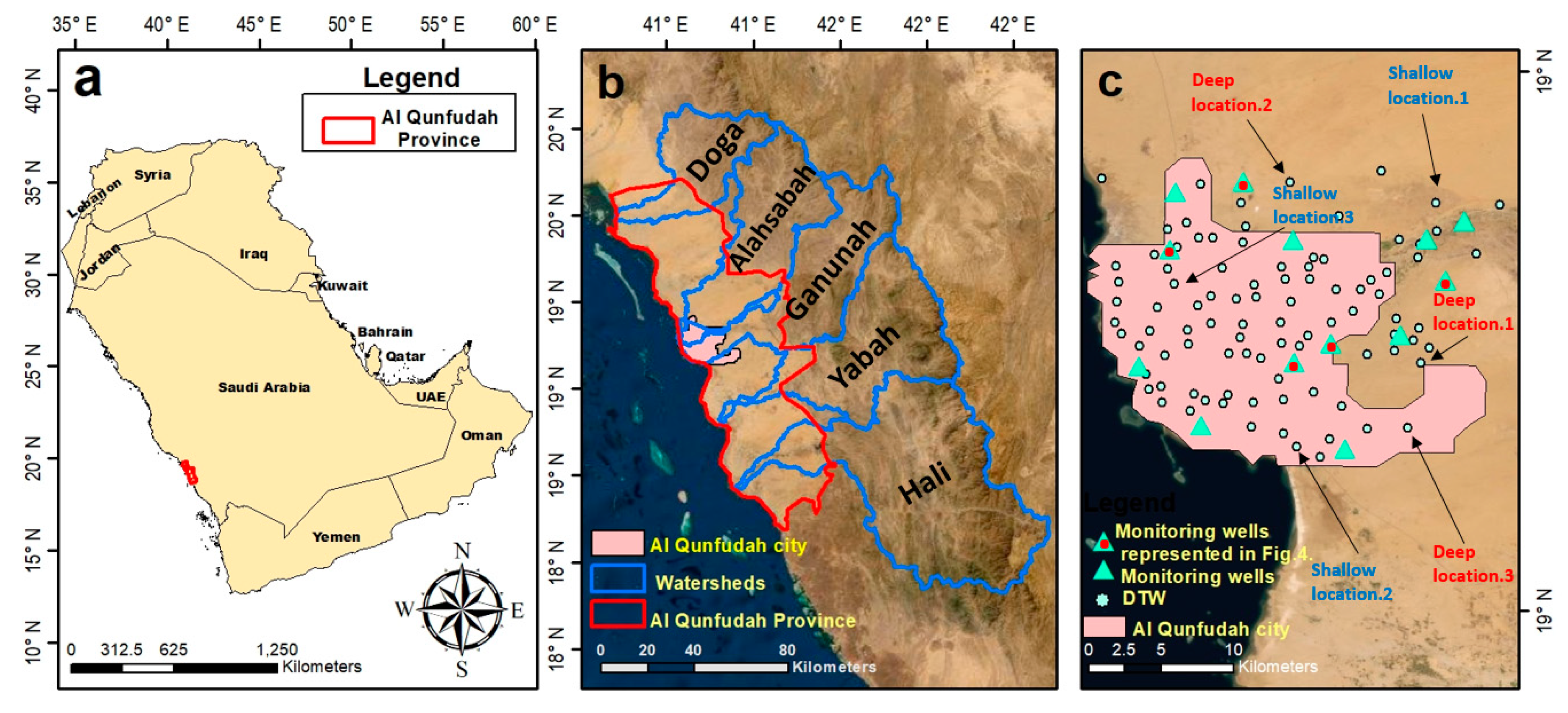
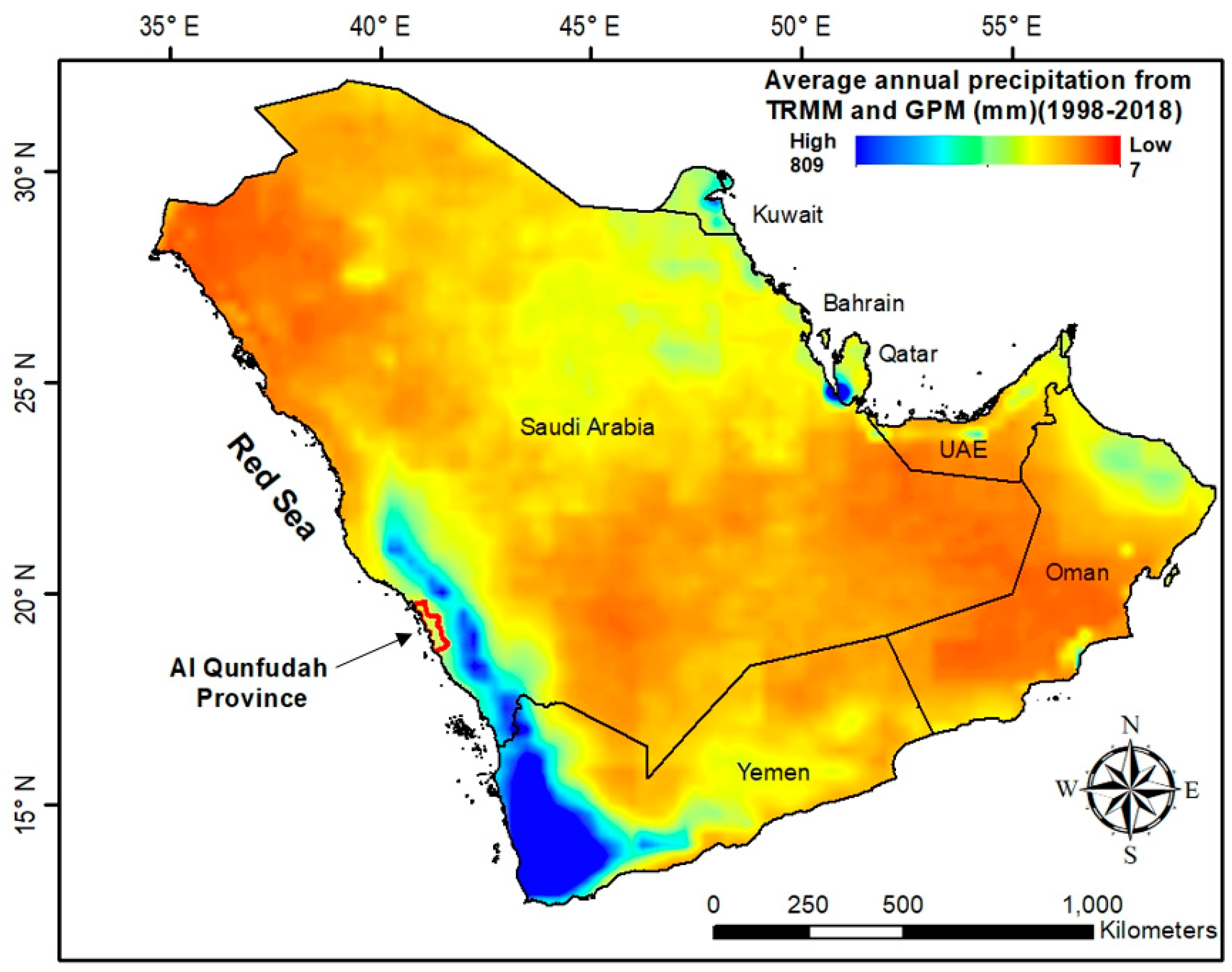
37]. The study area (Al Qunfudah Province) is located within the eastern coastal plain of the Red Sea in southwest Saudi Arabia and is part of the Asir mountainous region, which runs parallel to the Red Sea (
Figure 1). The Asir region receives the highest average annual precipitation (AAP) in the Kingdom of Saudi Arabia (400–700 mm yr−1) [
38] (
Figure 2). A number of cities are located within the Red Sea coastal plain, including the major city of Al Qunfudah and surroundings (area: 294 km
2), with a population exceeding 300,000. This city is apparently built along one of the main channels draining a large (2299 km
2) watershed, namely the Ganunah watershed (
Figure 1b). The main channels are subject to flooding during high precipitation events [
12] and are often the sites of organized agricultural development. The city of Al Qufudah is developed on alluvial fan deposits, where there is a 1%–2% elevation gradient of the ground surface that increases from sea level to more than 100 m above mean sea level within 5–10 km east of the Red Sea coastline.
Over the last few years, damage arising from elevated groundwater levels has been reported from several parts of southwestern Saudi Arabia. This include rising groundwater that flooded basements and submerged sewer pipes and utility lines in some areas [
39]. Temporal head data from 13 monitoring wells within Al Qunfudah city and surroundings (
Figure 1c) reveal a rise in water levels by up to 2 m since 2017.
3. Materials and Methods
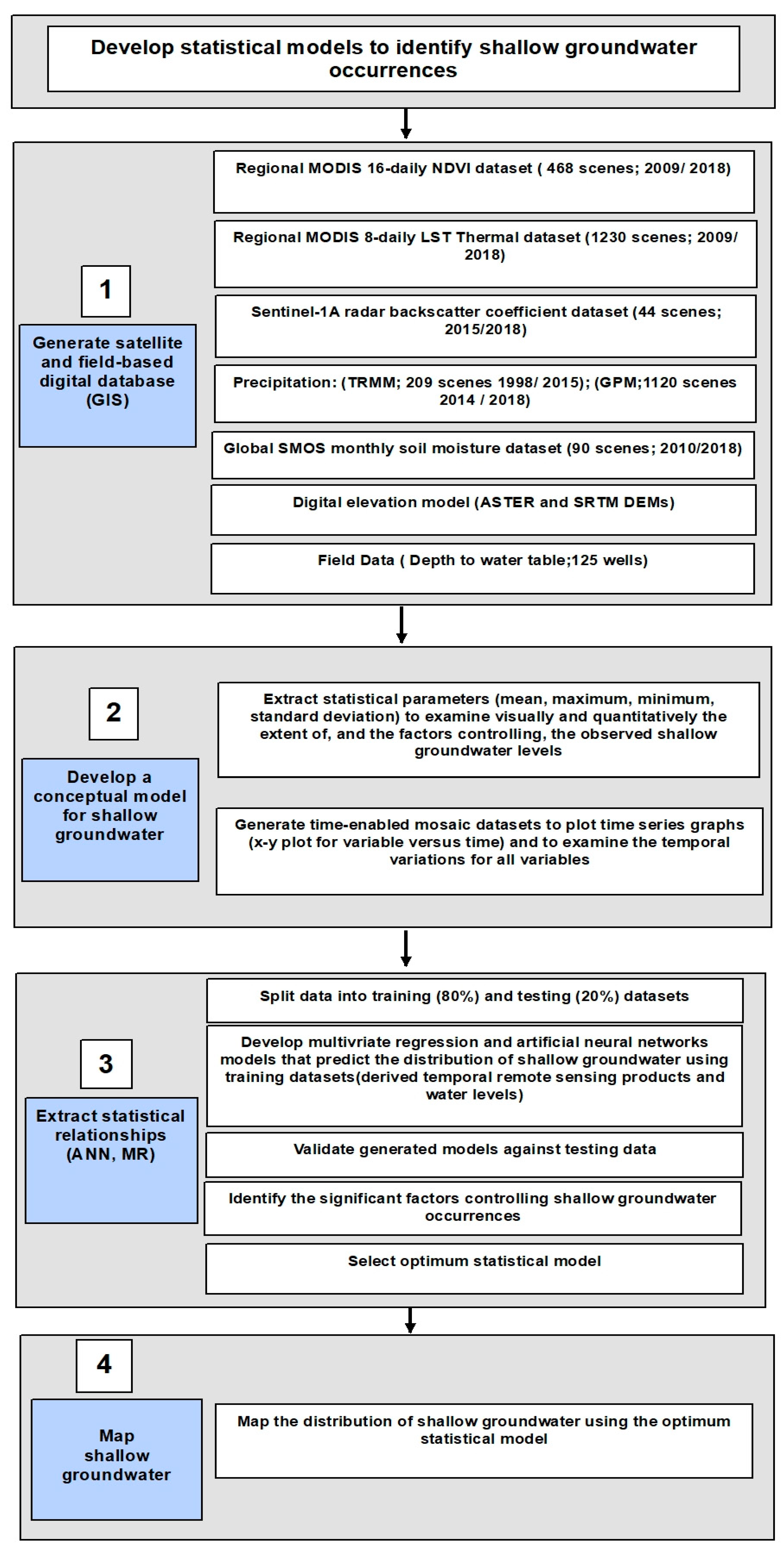
We accomplished the goals described above through the identification of areas experiencing shallow groundwater, by developing multivariate regression (MR) and artificial neural networks (ANN) statistical models over Al Qunfudah city and surroundings where field observations (DTW) are available. An inventory was compiled for a report by the Saudi Geological Survey on the occurrences of areas witnessing shallow groundwater levels in the coastal zone of Al Qunfudah. The statistical relationships relate the field observations to remotely acquired data sets. The adopted procedures involved four major steps: (1) constructing a digital database (GIS) to host relevant geologic, hydrogeologic, topographic, land use, climatic, and remote sensing data sets; (2) developing and testing a conceptual model that explains the observed spatial and temporal correlations between the individual variables and the target variable (shallow groundwater); (3) constructing and validating statistical models to map the distribution of shallow groundwater occurrences using MR and ANN over Al Qunfudah city and surroundings; and (4) using the optimum statistical model to map the distribution of shallow groundwater occurrences across the entire Al Qunfudah Province (
Figure 3). In the development of the conceptual model, we examined whether remotely acquired observations over areas characterized by shallow groundwater are different from those acquired over deep groundwater. We also examined whether there are larger variations in these variables over areas characterized by shallow groundwater, compared to others characterized by deep groundwater. The remote sensing data included NDVI, LST, SMOS, and global precipitation measurement (GPM) measurements as well as Sentinel-1A RBC.
3.1. Construct a Digital Database (GIS) to Host Relevant Datasets
The first step involved the generation of a GIS to host all relevant datasets that could be used for the identification of areas of shallow groundwater and the factors controlling this phenomenon. These include the temporal and spatial remote sensing products and field datasets. This step involved collecting field data (e.g., DTW; number of wells: 125) and downloading and processing temporal visible and near-infrared (VNIR), thermal, radar, precipitation (GPM), and SMOS data sets to compute LST, NDVI, soil moisture, precipitation, and RBC. In this section, we also explain the response of the selected remote sensing measurements in areas of shallow groundwater.
3.1.1. Identify DTW as Target Data
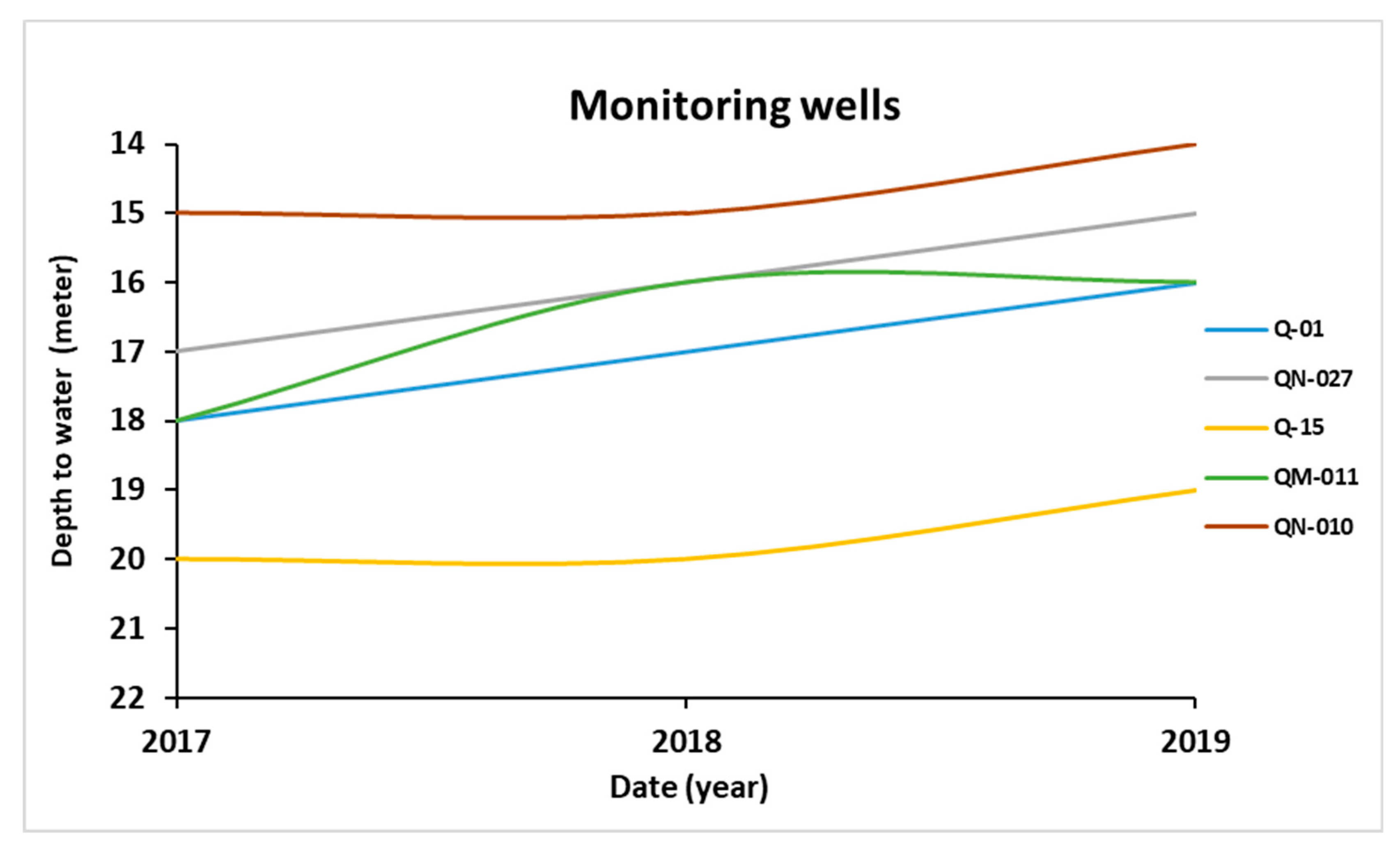
The Saudi Geological Survey conducted an intensive drilling project, drilling 125 wells over Al Qunfudah city and surroundings in 2016. Following the completion of the drilling project for the wells, the DTW was measured for each of the drilled wells during a period of few weeks during the months of October and November. In the construction of the statistical models, the DTW was used as the target variable, which was the average of measurements taken over a few weeks. Temporal measurements for the water table were available for a limited number of wells (13 wells), all of which had a reported rise (1 to 2 m) in groundwater level throughout the period 2017 to 2019 as shown in
Figure 4, which shows the rise in groundwater level in five of these wells over the past three years. The reported DTW for each of the years between 2017 and 2019 are averages of several measurements (3–4 measurements) for each well.
3.1.2. Potential Impact of DTW on NDVI
The NDVI data product (spatial resolution: 250 m), acquired by the National Aeronautics and Space Administration (NASA) MODIS satellite, was utilized in this study. The data were downloaded from NASA’s Vegetation Index processing website (
https://modis.gsfc.nasa.gov/). The MODIS vegetation index images are produced at 16-day intervals at multiple spatial resolutions. They provide consistent spatial and temporal comparisons of vegetation canopy greenness, leaf area, and chlorophyll and canopy structure. The ArcGIS Marine Geospatial Ecology Tools (MGET;
https://mgel.env.duke.edu/mget/) was used to convert Hierarchical Data Format (HDF) format to GeoTiff format. The MODIS NDVI data has been used in a broad range of research activities, such as drought monitoring, global vegetation variation, and agricultural and hydrologic modeling [
40,
41,
42]. In arid and semi-arid areas, climate change and water availability are vital factors affecting vegetation dynamics [
43,
44]. In arid and semi-arid environments, the DTW has been identified as an important factor affecting the vegetation cover [
31,
45]. In areas characterized by shallow groundwater, but not in others with deep groundwater, the root zones of vegetation reach the water table. Studies have shown that, in the arid regions, the root zones of the natural vegetation reach a depth of 2–7 m [
46,
47,
48].
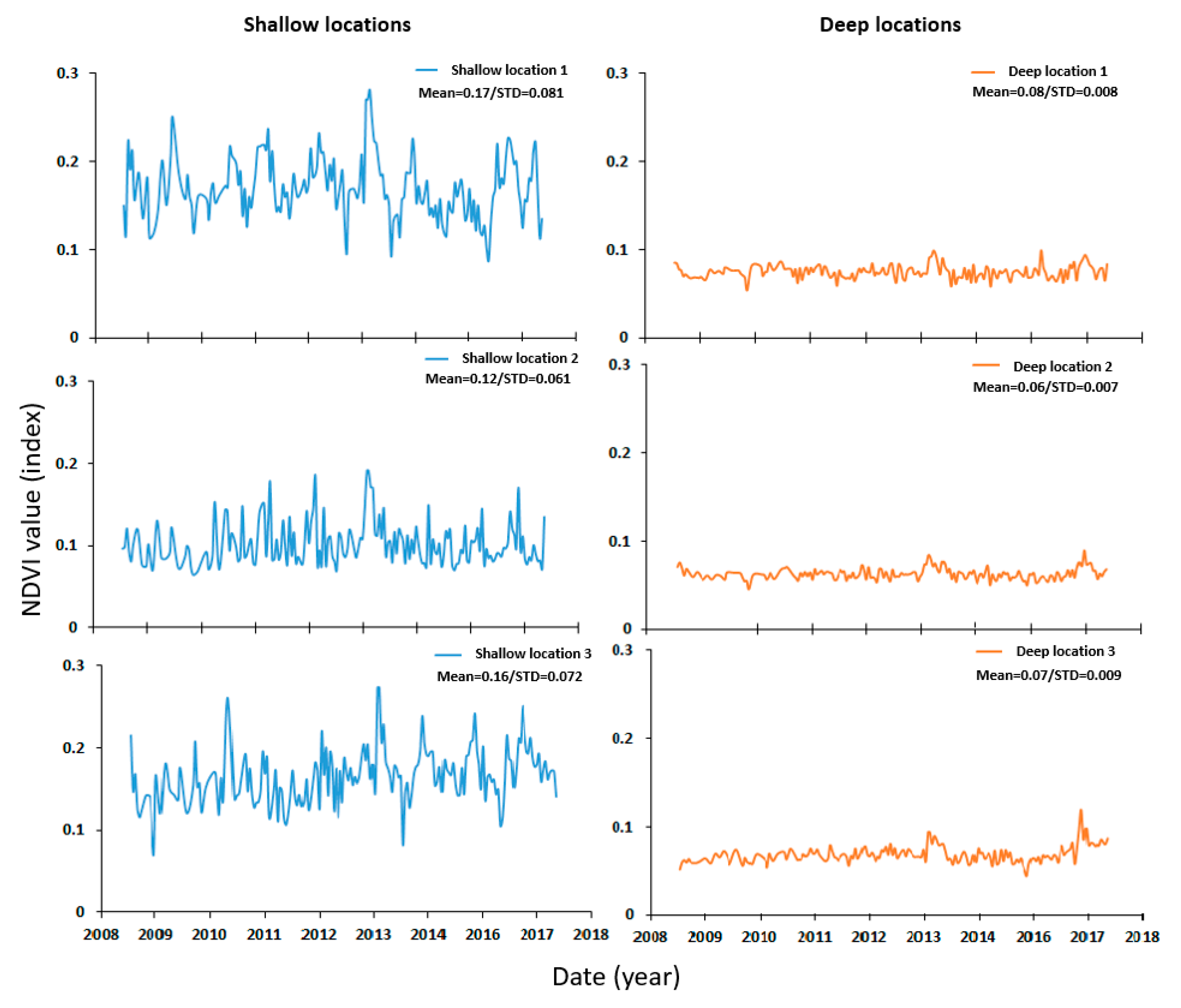
The DTW and NDVI relationship was investigated. Thereby, an average NDVI image and a STD image was extracted over each of the investigated wells by averaging the NDVI values from images acquired over the period 2015–2018. We averaged multiple NDVI images to capture the vegetative density of each pixel throughout the investigated period instead of using a single NDVI image, which might represent spatial vegetation variations relative to a specific season of a particular year. If the vegetation was supported by shallow groundwater, we expect higher NDVI values and higher variations in NDVI values. These variations are represented by higher STD values in response to seasonal and inter-annual fluctuations in groundwater levels. Over areas characterized by deep groundwater levels, vegetation will be absent since the roots will not reach the groundwater table and will not be affected by fluctuations in water levels. In some of the arid to semi-arid areas worldwide, vegetation can be maintained by precipitation. However, the former, but not the latter, scenario is more likely to occur in our study area given the paucity of precipitation events.
3.1.3. Potential Impact of DTW on LST
We used the LST (Kelvin) 8-day data product (spatial resolution: 1000 m) acquired by NASA’s MODIS Aqua satellite. The data was downloaded from the LST processing website (
https://modis.gsfc.nasa.gov/), which provides an option for periodic data download for specified regions via a free data subscription service. The MGET package was used in an ArcGIS environment to convert HDF format to GeoTiff format. LST has been used extensively in multiple research disciplines including global climate, agriculture, hydrology, and ecology [
49,
50]. Many of these studies have shown that vegetation intensity is inversely correlated with LST, where increases in vegetation are accompanied by reduced LST [
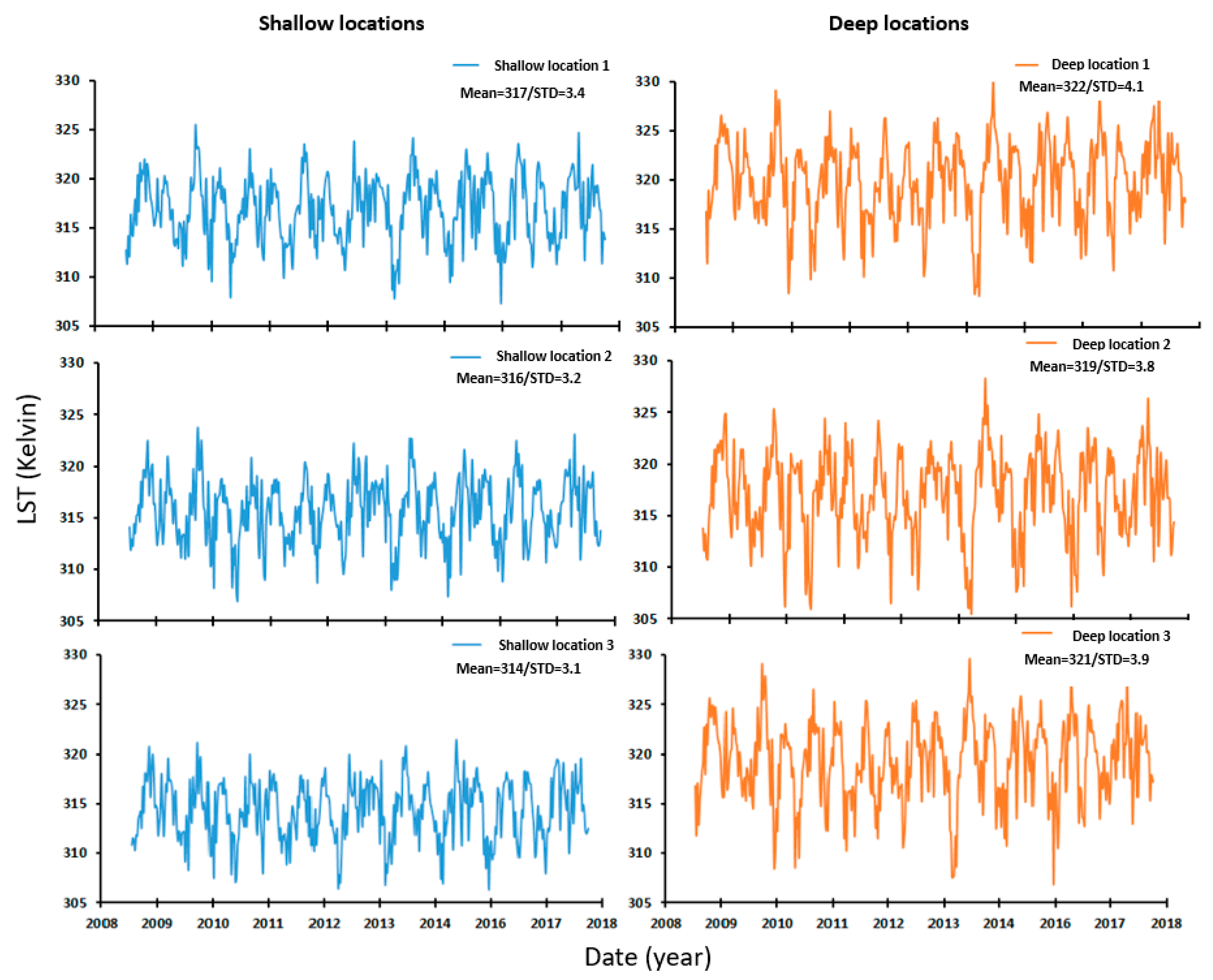
51]. An average LST image was extracted over each of the investigated wells by averaging the LST values from images acquired over the study period (2015–2018), and an STD LST image was extracted as well. Over areas of shallow groundwater, we expect low LST and less variations (i.e., low STD) in response to seasonal and inter-annual fluctuations in groundwater levels, and vice versa over areas with deep groundwater. The advocated model holds true for shallow groundwater and does not necessitate the presence of water at the surface.
3.1.4. Potential Impact of DTW on RBC
Sentinel-1 is a satellite mission of the European Space Agency (ESA) that uses synthetic aperture radar (SAR) operating in the C-band wavelength region (spatial resolution: 12 m). Sentinel-1A radar ground range detected (GRD) scenes were downloaded for ascending acquisition modes from Sentinel Data (
https://asf.alaska.edu). Ascending acquisition modes were selected due to the availability of scenes covering the study area. The following operations were conducted: co-registration, radiometric calibration and calculation of radar backscatter coefficient (beta naught [β
0]) in decibels [
52,
53], speckle filtering, terrain flattening, and geometric correction. RBC has been found to be effective in monitoring hydrologic systems including seasonal patterns of flooding [
54,
55]. Average and STD images were generated from the temporal β
0 images acquired over the investigation period (2015–2018). Over areas of shallow groundwater, we expect that the β
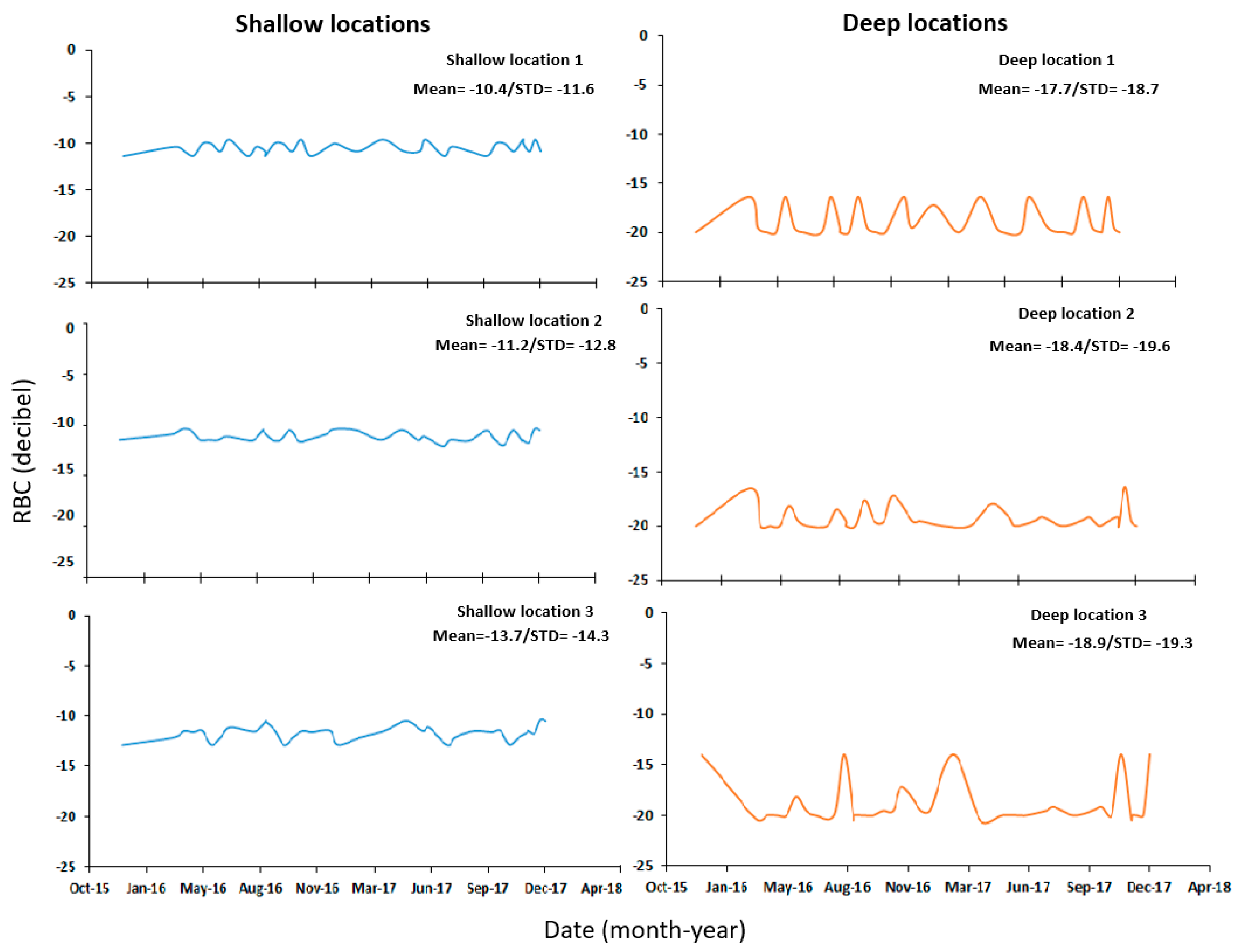
0 values will be high and vary in magnitude (i.e., high STD) in response to seasonal and inter-annual fluctuations in groundwater levels and vice versa over areas with deep groundwater.
3.1.5. Potential Impact of DTW on Soil Moisture
ESA’s SMOS Earth Explorer mission is a radio telescope in orbit pointing towards the Earth. The microwave imaging radiometer using aperture synthesis (MIRAS) radiometer on this mission picks up faint microwave emissions from Earth’s surface to map levels of land soil moisture and ocean salinity. SMOS monthly data (spatial resolution: 0.27° × 0.27°) for ascending acquisitions was downloaded from the Centre Aval de Traitement des Donnees SMOS (CATDS) website (
https://www.catds.fr/Products/Available-products-from-CPDC) using FTP Filezilla software. The MGET package was used to extract soil moisture images from the netCDF format, then re-project and export the output in GeoTiff format. The SMOS data, excluding pixels over the sea, was interpolated using the centers of the neighboring pixels to extract data values at finer scales. In doing so, linear variations between neighboring pixel values were assumed. An average and an STD image was generated from the SMOS images acquired over the investigation period (2015–2018). Over the areas of shallow groundwater, we expect the soil moisture values to be high and vary in magnitude (i.e., high STD) in response to seasonal and inter-annual fluctuations in groundwater levels and vice versa over areas with deep groundwater.
3.1.6. Potential Impact of Precipitation on DTW
The GPM mission is a network of satellites which provides global observations on the distribution and intensity of precipitation in the form of rain and snow. The GPM data is helping advance our understanding of Earth’s water and energy cycle and is providing accurate and timely information of precipitation to address societal needs [
56]. Precipitation is the driver of all hydrologic systems; an increase in precipitation increases runoff, surface water levels, groundwater infiltration, and storage, and leads to a rise in water table [
57,
58]. In this study, GPM (IMERG Final Precipitation L3 Half Hourly (spatial resolution: 0.1° × 0.1°)) daily products were downloaded from the GPM website (
https://pmm.nasa.gov/data-access/downloads/gpm) covering the period of 2015 to 2018. With increased precipitation, one should expect shallowing of DTW.
3.2. Development and Validation of a Conceptual Model for Shallow Groundwater
As described in the previous section, we expect to observe high NDVI, high radar backscatter, high soil moisture, and low LST and relatively large variations in each of these variables (except LST) over areas of shallow groundwater and vice versa over areas characterized by deep groundwater.
Following the downloading and processing of the remote sensing products, we tested the merits of our conceptual model by: (1) applying statistical parameters (e.g., mean, maximum, minimum, STD) for all of the digital datasets using cell statistic tools in ArcGIS, and (2) generating time-enabled mosaic datasets and plotting time series graphs (X–Y plot for variables versus time) to examine the temporal change for all variables. Uniformly spaced grid points were used to extract the values from products of different resolutions, and subsequent processing was done on the same grid to achieve computational efficiency. The collected remote sensing products were later checked for consistency and significance.
Six locations were selected: three characterized by shallow groundwater levels (DTW: ≤5 m) and three by deep ground water levels (DTW >5 m) for the purpose of examining whether the areas characterized by shallow groundwater would have a response on one or more of the selected image types (e.g., NDVI, RBC, and LST images, as well as the STD of each of these images) that is different from that over areas of deep groundwater (
Figure 5,
Figure 6 and
Figure 7). The locations for these six wells are shown in
Figure 1c. Comparisons of the temporal (2009 to 2018) variations in NDVI values between the three shallow and the three deep groundwater wells are shown in
Figure 5, and comparisons for the variations in LST for the same six wells over the same period are shown in
Figure 6. The comparisons for the backscatter coefficient variations over a shorter time period (2015 to 2018) are given in
Figure 7. The shorter temporal coverage is attributed to the period of operation of the Sentinel-1A mission and scene acquisition dates over the study area (launch date: 2014; first acquisition over study area: 2015).
3.3. Construction and Validation of a Statistical Model to Map Shallow Groundwater Occurrences
3.3.1. Screening of the Variables
The first step for the construction of the statistical model was to identify the variables to be considered for model development and to determine the optimum combination of significant variables. The screening of variables was conducted using exploratory and stepwise regression. The correlation coefficients for these variables are shown in
Table 1. This step gives first-hand insights into the contribution of each variable to the dependent variable (DTW). Only the variables identified as being significant were considered for the statistical model.
We conducted exploratory and stepwise regression and investigated the p-value and R² values to determine their significance. We experimented with normalized and non-normalized values to determine which of the two datasets provided the optimum results. During the process, we retained the variables with low
p-value and high R² values. These were considered as being of higher significance and as having a stronger ability to explain the variability of the dependent variable. Following the significance test, the variables were subjected to multicollinearity test using the variance inflation factor (VIF) values [
59]. A variable with VIF higher than 7.5 was considered redundant with the second highest VIF and was omitted. This step was performed for all the redundant variables by dropping one variable at a time without reducing the overall performance of the model. The redundancy test was conducted iteratively to ensure that significant and non-redundant variables were not eliminated. Our goal of this exercise was to obtain the highest overall R² value (0.67) with a minimal number of significant variables. Only six variables (GPM, LST, NDVI, RBC, STD of LST, and STD of NDVI) were shortlisted for further consideration as shown in
Figure 8. Although not initially incorporated, topography was a potential factor, yet we quickly realized that the topography showed very little variation over the training site (Al Qunfundah city and surroundings; refer to
Figure 1c). The relative significance of each of the short-listed variables was obtained using the normalized data set.
3.3.2. Identification of the Optimum Model
Two statistical approaches, MR and ANN, were adopted to model the relationships between the shortlisted input variables and the response variable. The training subset comprised 80% of the total data points and was used to construct the model, whereas the remaining 20% were used to evaluate the performance of the models and were not used for model development. The same sets (training and testing datasets) were used for model development and validation of the MR and ANN models.
3.3.3. Multivariate linear regression
The MR method describes a multivariate linear relationship between one or more predictor variables and a response variable [
60]. The model assumes that the magnitude of the dependent variable is represented by the sum total of all the contributions of the individual variables; any unexplained contribution is represented by a model bias or a constant. The regression line for
n independent variables
X1,
X2,
X3,...
Xn can be expressed as follows:
where
Y is the predicted value of the target variable,
A0 is the model bias and
A1 through
An are individual model coefficients. The Spatial Statistics extension in ArcGIS was used in this analysis.
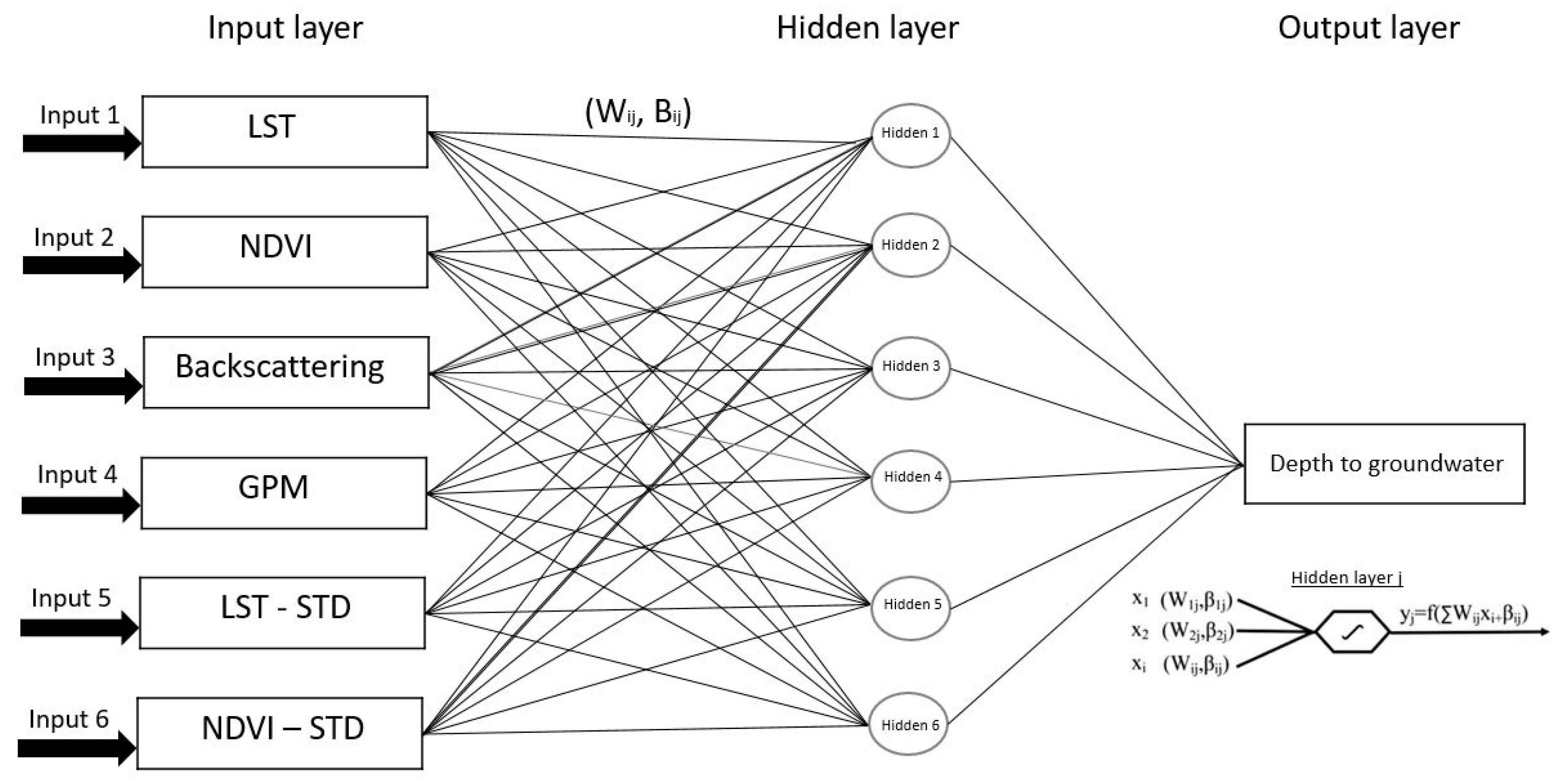
3.3.4. ANN Model
ANN utilizes algorithms to model the complex and non-linear relationships [
61,
62] among various factors controlling the response variable, in our case the DTW. The ANN is based on connection of neurons, a process that is designed to replicate the functions of neurons in the nervous systems of organisms; they pass information between one another, a structure that enables ANNs to be trained and to learn complex interactions. A fitting neural-network module of MATLAB
R2019 was utilized to detect shallow groundwater.
A simplified flowchart of our constructed ANN model is provided in
Figure 9. The hyperparameter that controls the model structure (e.g., number of layers, number of hidden neurons, and number of epochs) was set before the learning process was conducted. An error technique was applied to determine the optimal number of hyperparameters; this was accomplished by gradually adding the number until the predicted and observed values begin to mimic each other. The model performance was evaluated using the mean squared error (MSE) performance function where minimum MSE was achieved for the testing datasets. The widely used backpropagation learning algorithm [
62] in a fitting neural-network modeling was applied and the number of hidden neurons was increased until the model performance plateaued at 6 neurons to prevent overfitting of the model. The model was optimized for absolute value of DTW to allow validation with both DTW and classified binary values for shallow and deep groundwater.
3.4. Selection of the Optimum Model to Map Shallow Groundwater across Al Qunfudah Province
Following the development of the MR and ANN models, their performance was assessed and the model with the highest performance was used to map the distribution of shallow groundwater throughout the Al Qunfudah Province.
4. Results
Findings from the exploratory and stepwise regression investigations revealed that SMOS was redundant with RBC (correlation coefficient: 0.89;
Table 1.), possibly because radar backscatter is controlled at least in part by soil moisture [
63]. SMOS data sets were removed from further consideration, and RBC was preferred over SMOS because of its higher spatial resolution. The STD of RBC was found to be less significant than the remaining variables and was dropped as well. The elimination of SMOS and STD of RBC did not affect the overall performance of the model. Out of eight variables under initial consideration, only six variables (LST, NDVI, RBC, GPM, STD of LST, and STD of NDVI) were shortlisted for model construction (
Figure 8). The relative significance of each of the short-listed variable set is given (in percentage) in
Table 2. LST was found to be the most significant variable (43.2%), whereas each of the remaining five variables accounted for 9%–15% of the observed variations in the response variable.
Each of the determining variables exhibited a unique response to the DTW as shown in
Table 3. The table lists the MR coefficients for each variable in predicting DTW. The sign (±) in front of the coefficient for each selected variable indicates the nature (positive/negative) of the relationship between the variable in question and the response. As expected, in areas experiencing shallow groundwater, soil moisture increases, causing an increase in RBC and a decrease in LST and in its variability (STD of LST). One would also expect an increase in NDVI and in its STD in areas characterized by shallow groundwater. This is true for the STD of NDVI, but not for the mean of NDVI.
As expected, the MR and ANN yielded different levels of accuracies (
Table 4) due to the inherent differences in these models (linear versus complex relationships). Both models yielded high accuracy in predicting the target with a slight enhancement of the ANN (accuracy: 92%) over the MR model (accuracy: 88%). The prediction accuracy was based on the ability of the model to predict shallow (≤5 m) and deep groundwater (>5 m); six variables (LST, NDVI, RBC, GPM, STD of LST, STD of NDVI) were used by both models for prediction purposes. In both cases, inclusion of additional variables did not improve the model accuracy. Although both models performed equally well, the ANN had a slight advantage over the MR model. The ANN apparently better accounted for the complex interactions among the variables and better explained the variability in the response variable. This suggestion is supported by the lower root mean square error (RMSE) for the ANN (14.93) compared to the MR (15.31) as shown in
Table 4. It should be noted that the RMSE values in
Table 4 were computed using the testing datasets (20%).
For demonstration purposes, we used the ANN model that was developed over Al Qunfudah city and surroundings (area: 294 km
2) to map shallow groundwater across the entire Al Qunfudah Province (area: 4680 km
2;
Figure 10). The generated ANN model output (derived matrix) was utilized in an ArcGIS 10.6 platform for mapping the distribution of the shallow groundwater occurrences across the province.
5. Discussion
The prediction of DTW in our study area involves developing an understanding of the variables indicative of the presence of shallow groundwater and the complex interactions among these variables. A conceptual model was first developed that predicts areas with shallow groundwater indicated by high NDVI (mean and STD) and RBC (mean and STD) values and low LST (mean and STD) compared to areas with deep groundwater. This model was tested visually over 13 locations and was then validated and refined using an exploratory stepwise regression analysis. Six of the eight variables were selected and two were omitted given their lower significance and/or redundancy. An MR model was developed to determine the level of variance each variable explains in the response variable and the nature of the relationship between shallow groundwater occurrences and the individual variables.
The MR model was used to determine the comparative significance of each variable towards the DTW. Although simplistic, this information provided first-hand insights into the contribution of each variable. These estimated contributions represent the minimum contribution of each variable and do not reflect the complex interaction among variables which could be significant in natural environments. Inspection of
Table 2 reveals that the most significant (43.2%) variable is the LST (mean), whereas the remaining five variables have sub-equal significance (range: 9.2%–15.4%). These include NDVI (mean and STD), RBC (mean), and precipitation. Although SMOS data sets appeared to be significant, it was redundant with RBC, and thus it was dropped. Similarly, the STD of the RBC was dropped from the model because it did not enhance the model performance. This may be because radar backscatter is already explaining the variance present in dependent variable.
The MR model was used to infer the nature of relationship between the independent variable and the DTW. The information provided in
Table 3 can be used to interpret the nature of the relationship between the DTW and the individual variables. In simple terms, the mathematical sign (±) associated with each coefficient provides the information about the type of the response it offers to DTW. For example, areas of shallow groundwater (low DTW) are characterized by relatively low LST (mean, STD), high RBC (mean), high variation in NDVI (STD), and high precipitation compared to areas characterized by deep groundwater (high DTW). With the exception of the NDVI (mean), these observations are consistent with our conceptual model and with the visual inspection of the temporal variations over the 13 test wells (
Figure 1c and
Figure 4). The NDVI (mean) shows a decrease in NDVI value in areas of shallow groundwater and vice versa for deep groundwater. One possible explanation for this discrepancy is the assumption that all the observed temporal and spatial variations in NDVI are caused by variations in the intensity of natural vegetation. While this assumption is true over much of the desert landscape, it does not necessarily apply over farmed areas where groundwater could be extracted from deep or shallow depths. Also, locally within the desert landscape, there are areas which receive more of the sporadic flash floods and could maintain a vegetative cover throughout many months of the year. Examples include the main valleys that collect runoff from extensive areas within basins or sub-basins. Over these irrigated areas and those areas that receive more of the sporadic precipitation events, the NDVI values could be high, yet the DTW is not necessarily shallow.
Regardless of whether MR or ANN model was used for prediction purposes, the DTW was better predicted for the shallow groundwater compared to the deep groundwater. For the MR model, the RMSE for shallow groundwater was 6.67 and 18.77 for deep groundwater. Similarly, for the ANN model, it was 6.16 and 18.54 for the shallow and deep groundwater, respectively. This is to be expected given that the effects of groundwater on vegetation intensity, LST, RBS, and soil moisture are felt at near surface levels, decrease with depth, and are not captured beyond a certain depth (in our case 5m) by remote sensing observations. In other words, both the MR and the ANN models could be used to predict the absolute value of the DTW in the case of the shallow groundwater, but not the deep groundwater. This is the reason we displayed the model outputs in a binary format. The ANN provided enhanced prediction over the MR model (
Table 4) and thus, it was selected for mapping the distribution of shallow groundwater across Al Qunfudah Province. This is to be expected given that the ANN models can account for the variations in data distributions and patterns and can even consider the smallest and least obvious fluctuations in data sets [
64,
65].
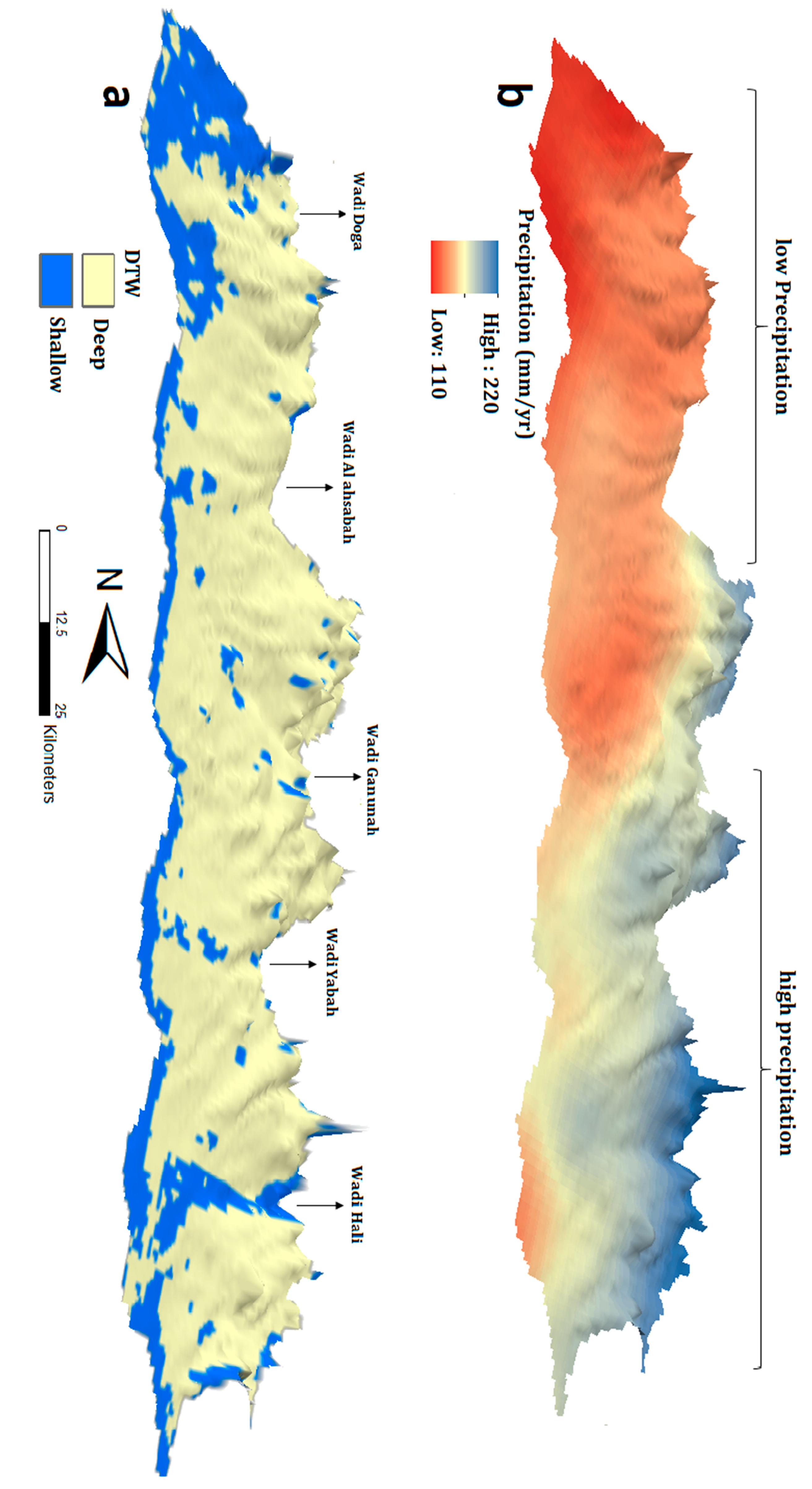
The developed statistical model for the DTW across Al Qunfudah Province does not explain the observed rise in groundwater levels over the past three years (
Figure 4). We address this issue by examining spatial and temporal variations in precipitation patterns over Al Qunfudah Province. We created 3D renderings of the generated binary DTW (
Figure 10a) and AAP (
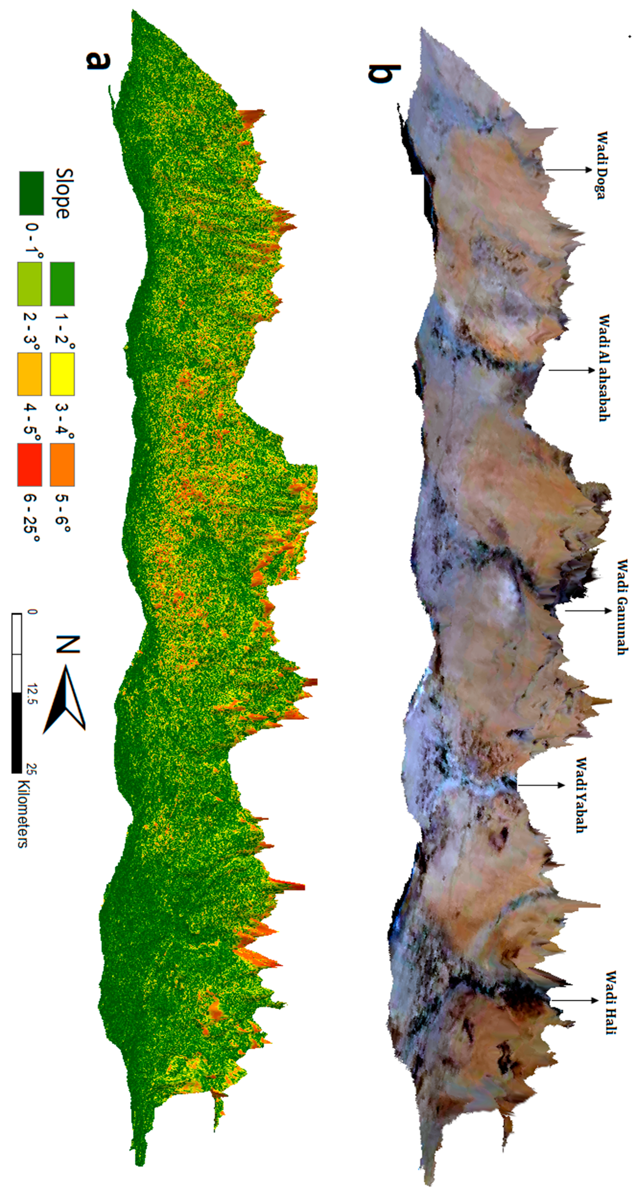
Figure 10b) each draped over the digital elevation model (DEM) that was extracted from the advanced spaceborne thermal emission and reflection radiometer (ASTER) image. Additional 3D renderings were generated for a slope image DEM (
Figure 11a) and a natural color composite [
66] map (
Figure 11b) each draped over the DEM. Inspection of
Figure 10 and
Figure 11 reveal some general features. Shallow groundwater is found along the coastal plain in areas proximal to the coastline (width: 3–5 km) and within the main valleys that collect runoff from precipitation over the Red Sea Hills. The most prominent of these main valleys is the east-west trending Wadi Hali. The Wadi Hali catchment receives higher precipitation (AAP: 192 mm/yr) than those to the north (AAP: 152 mm/yr.) (
Figure 10b). This could explain why Wadi Hali, but not Wadi Ganunah and Wadi Doga have shallow groundwater. Not only do the southern highlands receive higher precipitation, but the general slope of their coastal plain is also gentle (average slope: 2.5°) compared to the northern coastal plain areas (average slope: 6°;
Figure 11a). The steeper the slope, the less infiltration, and the deeper the groundwater.
We showed that the spatial variations in precipitation could explain at least in part the modeled variations in the DTW across Al Qunfudah Province, but it does not explain the observed rise in groundwater levels (
Figure 4). We address this issue by examining spatial and temporal variations in precipitation patterns over Al Qunfudah Province. Inspection of
Table 5 shows that there has been an increase in the AAP over Al Qunfudah Province over the past three years (2017–2019: 162 mm/yr) compared to the preceding three years (2014–2016: 139 mm/yr). The table also shows that there has been a similar increase in the AAP over the watersheds draining into Al-Qunfudah Province. In the years 2017–2019, the AAP was high (Hali watershed: 192 mm; Yabah: 170 mm; Ganunah: 163 mm, Al ahsabah: 158 mm; Doga: 152 mm) compared to the preceding three years (Hali: 171 mm; Yabah: 151 mm; Ganunah: 140 mm; Al ahsabah: 141 mm; and Doga: 127 mm). The increase in precipitation over Al-Qunfudah Province and over the watersheds that drain into the province will lead to increased infiltration and recharge of the alluvial aquifers underlying the Al-Qunfudah coastal plain causing a rise in groundwater levels in these aquifers. Thus, the observed increase in groundwater levels over the past three years (
Figure 4) is likely to be related to increased precipitation. Additional field, geochemical and modelling investigations are required to adequately address the factor(s) causing the rise in groundwater levels in the study area.
There are several limitations with the applied methodology. The developed models were developed for the coastal plain of the Al Qunfudah Province. Thus, it could potentially be applied to similar settings along the Red Sea Hills or elsewhere, but not to areas with different geologic and hydrologic settings (e.g., mountainous terrains). The spatial and temporal distribution of training data was limited in our models. Large spatial and temporal (seasonal or inter-annual) variations in DTW could affect the accuracy of the model. Like any other machine-learning model, the addition of more training data over larger areas and time spans will significantly improve the predictability and vice versa. Several of our remote sensing datasets (e.g., RBC or DEM) are available at high resolution (12–30 m), whereas others (e.g., SMOS, GPM) are very coarse (0.27° × 0.27°; 0.1° × 0.1°). In other words, we had to combine high-resolution with low-resolution datasets, a process that reduces the accuracy of our statistical model predictions. The predictability of the model can be improved by providing the higher spatial resolution products for precipitation and SMOS or by adopting robust downscaling techniques to downscale low spatial resolution datasets [
67].
6. Conclusions
This study focused on developing statistical models to identify shallow groundwater occurrences over large areas using readily available remote sensing datasets. We used the coastal zone of Al Qunfudah Province, southwest Saudi Arabia, as a test site. A conceptual model was developed over the Qunfudah city and its surroundings, where field data are available. The model predicts that areas characterized by shallow groundwater could have high NDVI (mean, STD), high RBC (mean, STD), and low LST (mean, STD) compared to areas with deep groundwater levels.
A comprehensive spatio-temporal database was constructed, and the conceptual model was validated visually using field data (water levels in 13 wells) and remote sensing data over these wells. We constructed ANN and MR models to map the distribution of shallow groundwater occurrences in the Al-Qunfudah city and surroundings, tested the statistical models against field data, and selected the optimum model (ANN) to map the DTW across the entire Al-Qunfudah Province. The statistical models were constructed using randomly selected training data sets (80% of the total), whereas the remaining data sets (20%) were used for testing purposes. Our findings indicated an enhanced performance for the ANN model (92%) over the MR (88%) in predicting the distribution of shallow groundwater. Temporal correlations of the groundwater levels and satellite-based precipitation suggest that the observed rise in groundwater levels in 2017–2019 are attributed to an increase in precipitation in these years compared to the previous three-year period (2014–2016).
Even though this project focuses on Al Qunfudah Province and its surroundings, the adopted approach can potentially be replicated over many parts of the arid world with a similar climatic, geologic, and hydrologic setting. The addition of more training data over larger areas and time spans will significantly improve the predictability of adopted machine-learning techniques such as ANN. The applications of such technologies are cost-effective and could have significant societal benefits. These include, but are not limited to, locating additional fresh water supplies over extensive arid areas worldwide and addressing environmental problems arising from an increase in groundwater levels that may cause environmental problems to populations and loss of properties (e.g., destruction of foundations, structures, etc.).

 ,
, 


