Article

A Pathway to the Automated Global Assessment of Water Level in Reservoirs with Synthetic Aperture Radar (SAR)

1
National Institute of Education, Nanyang Technological University, Singapore 637551, Singapore
2
Asian School of the Environment, Nanyang Technological University, Singapore 637551, Singapore
3
Institute of Energy and Environment, University of Sao Paulo, São Paulo 05508-060, Brazil
4
Department of Geography and Environmental Management, University of Waterloo, Waterloo, ON N2L 3G1, Canada
5
Earth Observatory of Singapore, Nanyang Technological University, Singapore 637551, Singapore
6
School of Geographical Sciences, Guangzhou University, Guangzhou 510006, China
*
Author to whom correspondence should be addressed.
Remote Sens. 2020, 12(8), 1353; https://doi.org/10.3390/rs12081353
Submission received: 1 April 2020 / Revised: 20 April 2020 / Accepted: 21 April 2020 / Published: 24 April 2020

Abstract

:
Global measurements of reservoir water levels are crucial for understanding Earth’s hydrological dynamics, especially in the context of global industrialization and climate change. Although radar altimetry has been used to measure the water level of some reservoirs with high accuracy, it is not yet feasible unless the water body is sufficiently large or directly located at the satellite’s nadir. This study proposes a gauging method applicable to a wide range of reservoirs using Sentinel–1 Synthetic Aperture Radar data and a digital elevation model (DEM). The method is straightforward to implement and involves estimating the mean slope–corrected elevation of points along the reservoir shoreline. We test the model on six case studies and show that the estimated water levels are accurate to around 10% error on average of independently verified values. This study represents a substantial step toward the global gauging of lakes and reservoirs of all sizes and in any location where a DEM is available.

1. Introduction

The search for renewable energy has resulted in a global proliferation of hydroelectric dams. Thousands of artificial reservoirs have been constructed in the last decade [1,2], including hundreds in river basins of international importance such as the Amazon (416) and Mekong (371) [3,4]. Artificial reservoirs represent a two–way issue for worldwide water demand because they can cause environmental impacts, yet are necessary for human water resource use. If not well planned and managed, they represent threats to species health and diversity, contribute to losses of fish and ecosystem services by affecting the penetrability of light within the water column and reducing the river connectivity, and may become sources of greenhouse gases [5,6,7,8,9]. They are also major sinks for sediment and nutrients in river systems along with wetlands and floodplains [10,11,12,13]. Yet, in the context of global water security, they are important resources for regional populations, help control flooding along rivers, and generate clean energy [14,15,16].
The lack of consistent gauging severely limits understanding of the water storage role of the reservoir, habitat changes due to reservoir construction and filling, and potential flooding risks. Water accounting is essential for establishing policies and procedures to ensure that regional or basin–scale water balance is maintained over time [17]. Between 1984 and 2015, 90,000 km2 of permanent surface water disappeared from the Earth’s surface due mainly to extraction for human use and increased evapotranspiration brought on by climate change, while reservoir filling mostly accounted for the 184,000 km2 of a new permanent surface water [18]. Yet, for much of the world, reservoir gauging is scarce, and often not readily available to the public.
Reservoir and lake water level monitoring is one of the critical objectives identified by the World Meteorological Organization (WMO) and Global Climate Observing System (GCOS). Globally consistent (in time and space) water level monitoring is crucial because lakes and reservoirs are proxies used to understand global climate change [19]. Their role also needs to be taken into account in hydrological and atmospheric models for better understanding the past and current impacts of climate change on the lakes and reservoirs dynamics, and also for predicting future climate impact on water resources [20,21]. However, it is not possible to measure water level variations globally based on ground measurements alone, and the development of a global database of the reservoir water level is incomplete. Thus, to address the goals of the WMO and GCOS, continued research on water level monitoring needs to continue to motivate current and future research.
Satellite altimetry is an important method for gauging reservoir water levels from space [19,22,23,24], but can only measure water levels along a fixed orbital track and, thus, is limited in geographical coverage. Moreover, altimetry can successfully gauge or measure the water level of only relatively large inland lakes, leaving a substantial portion of global reservoirs ungauged [25]. Although the Ice, Cloud, and land Elevation Satellite (ICESat) and ICESat–2 have measured water levels in smaller lakes, they have a 90–day repeat with shifting orbits and, thus, are not useful for continuous monitoring of reservoirs and lakes.
Synthetic Aperture Radar (SAR) methods have shown promise for gauging and measuring the water level in lakes and reservoirs [26,27], while wide–scale adoption of these methods by non–experts in remote sensing could be due to a perceived difficulty in understanding and using SAR data. Automated workflows using SAR data and techniques have been proposed. However, these have focused mainly on obtaining water extent [28,29] and flooding extent [30]. SAR–based flooding extent products are even available online [30]. Yet, only rarely have SAR products been integrated with other remotely sensed data sources to provide information on water levels [27]. Simple and clear procedures for leveraging the integration of these data are, therefore, lacking. Remote sensing techniques that do not use SAR have been used to estimate reservoir water level or storage variabilities, but are mostly limited to large lakes or require some field or ancillary knowledge [31,32,33,34].
Although approaches intersecting the lake surface extent with DEMs to extract elevation information have been published, they were focused either on a specific arid environment [35,36] or on a local scale based on airborne LiDAR or interferometric DEM processing [37,38,39]. In this case, we propose a method that allows users to estimate WL dynamics at nearly global scales by using a relatively simple geographic information science (GIS) workflow (included as Figure S1) solely based on operational remote sensing data. Therefore, this method should be an attractive option for environmental managers without expertise in remote sensing and will complement studies on flood mapping, nutrient and sediment storage, and human impacts on water supply.
In this paper, we present a simple method to estimate the water level (WL) variability of lakes and reservoirs of almost any size solely based on readily available operational remote sensing data, without need for ground–based or a priori data. Water level estimates are derived from SAR data, which, unlike optical sensors, are very weakly affected by cloud coverage, overlaid on a Digital Elevation Model (DEM). We tested our method on six recently built reservoirs distributed across different continents, and verified the results using altimetry–derived water levels with centimeter–scale precision [40]. We purposely chose reservoirs where altimetry data were available to validate our results. However, our method is not spatially limited to below–nadir water bodies and can be used for lakes of almost any size and in any location as long as it is covered by a DEM (approximately 86% of the global surface in the case of the Shuttle Radar Topographic Mission (SRTM)).

2. Data and Methods

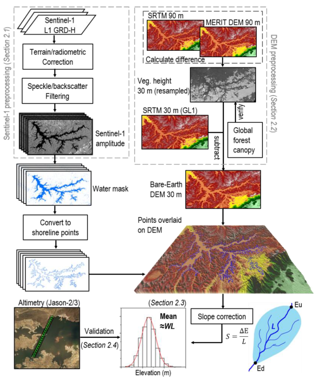
2.1. Sentinel–1 Data Acquisition and Preprocessing

We used SAR observations by the European Space Agency (ESA) C–band Copernicus Sentinel–1A and Sentinel–1B satellites for extraction of reservoir water masks (Figure 1). These satellites take images of the Earth routinely at a 12–day return period and generate high-resolution backscatter images that are made freely available by ESA. SAR is an active microwave sensor that is only weakly affected by the time of day or cloud cover, and the backscattering images have high contrast between land and water. Thus, SAR data are ideal for routine monitoring of water bodies such as the reservoirs and lakes.
We used Level 1 ground–range–detected high–resolution (GRD–HR) backscattering intensity products with VV polarization from Sentinel–1’s interferometric wide swath (IW) mode, downloaded from the Alaska Satellite Facility (https://www.asf.alaska.edu) (a total of N = 551 over six reservoirs). The data are provided in 250 km–wide swaths at 10–meter resolution, projected onto the WGS84 ellipsoid. To correct for topographic distortion due to the side–looking nature of the radar instrument, and to ensure precise co–registration with a Shuttle Radar Topography Mission (SRTM) digital elevation model, we orthorectified the images using ESA’s Sentinel–1 toolbox (http://step.esa.int/main/toolboxes/snap/). We first applied the precise orbit and radiometric calibration files from ESA, assembled along–track data slices as needed, and applied the terrain correction using the SRTM dataset before cropping the image to the target region.
To obtain and extract a water mask, Sentinel–1 images were first re–projected to the local UTM projected coordinate system. We used density slicing to extract water mask grids. Amplitude values of ≤0.036, defined through visual inspection and several simulations over different locations and dates, were used to denote water pixels. Thanks to the high contrast between permanent water and the ground surface along the reservoir edges, the method is not very sensitive to this value. To mask out brighter pixels that could result from back–reflection from the rough surface water (due to waves, wind, or rainfall), topographic shadowing on the land (e.g. Cao et al. 2019, Bolanos 2016) and instrumental noises such as speckles, we used a majority filter (3 × 3). Grids were then converted to polygons. We eliminated small polygons (<15,000 m2) outside of the area of the reservoirs. Reservoir polygons were then converted to line features, which consisted of multiple line patches. We only preserved line features longer than 1,000 m to efficiently filter line segments outside of the reservoir. The resultant trimmed line features define the reservoir shoreline. The noise filtering process described in this section is illustrated through an explanatory figure using a case of the Bansagar reservoir on 25 October 2017 (Figure 2).

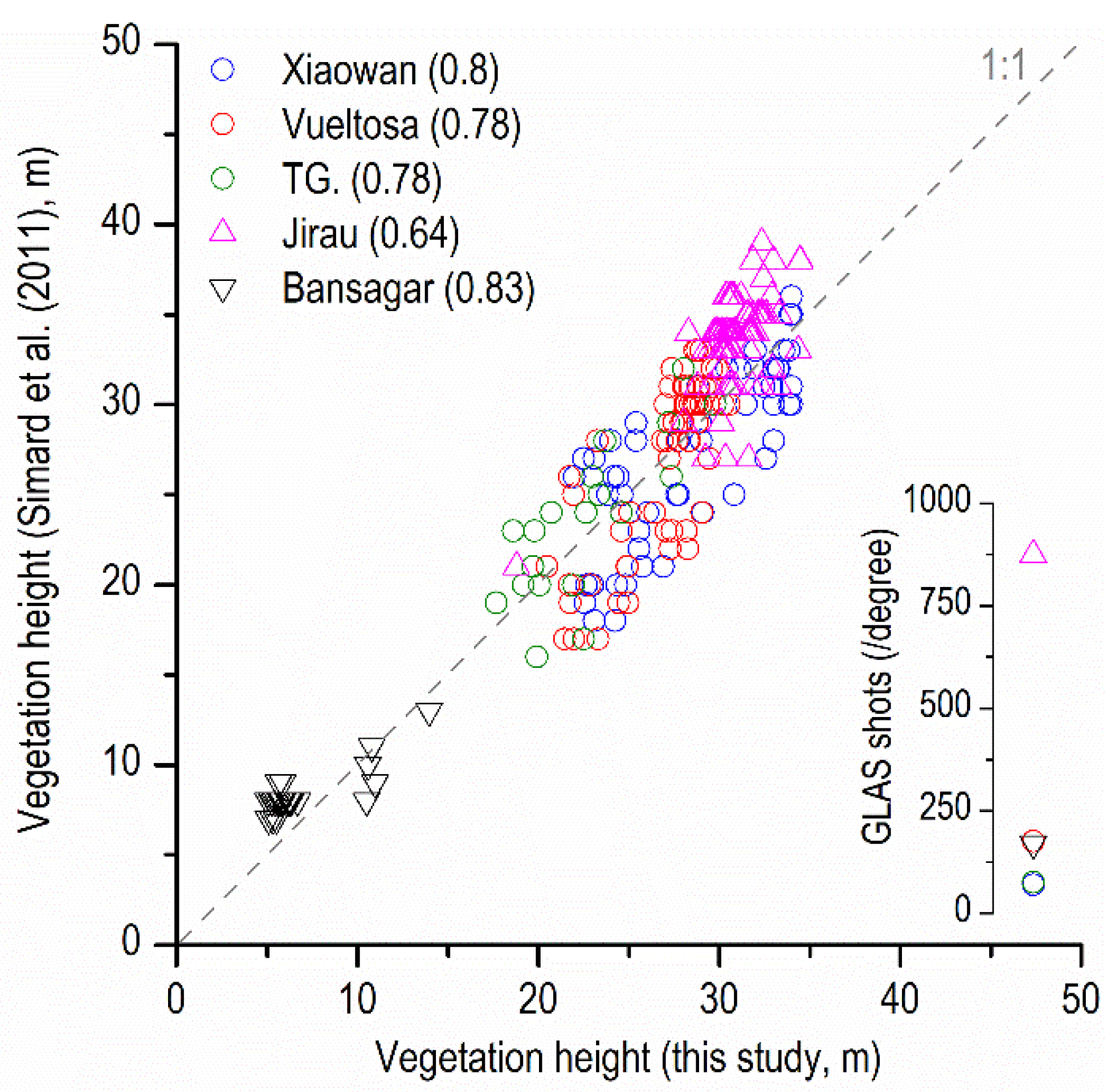
2.2. Digital Elevation Model (DEM) Processing and Validation

Our proposed gauging method used a combination of three global–scale DEMs to obtain WL: (I) Multi–Error–Removed Improved–Terrain DEM (MERIT DEM) [41], with 3–arcseconds resolution (90 m), (II) Shuttle Radar Topography Mission (SRTM) v4 [42] with 3–arcseconds resolution, and (III) SRTM GL1N v003 1–arcsecond resolution (30 m) [43]. MERIT DEM is a surface model with vegetation canopy removed, which considerably improves resultant topography accuracy. To improve upon the spatial resolution of the MERIT bare earth DEMs, we subtracted the corrected v4 of the SRTM 90 m (with vegetation), from the MERIT DEM (without vegetation). Although an issue has been raised concerning the SRTM V4 hole–filling method in flat areas around lowlands and large rivers [41], most reservoirs (including those in our study) are constructed in relatively high relief or mountainous terrain. In addition, since the reservoir WL gradually changes over the large impounded water body, the effect of void errors is considerably decreased when the reservoir size increases (see next section). Nevertheless, a discussion of the merits of different global–scale DEMs is beyond the scope of this study.
The "vegetation height" raster (90-m resolution) was generated and then verified against the global forest canopy height data at 1 km [44]. We resampled the vegetation height raster to 1 km using a bilinear interpolation method, and random points within the maximum extent of reservoirs were generated for the tree height comparison. The number of random samples was defined by the size of the reservoir (approximately one per 1 km2). We then resampled the "vegetation height" into 30-m spatial resolution pixels for subsequent subtraction from the SRTM 30-m dataset. The final DEM, thus, has 30-m spatial resolution with the vegetation effects removed.

2.3. Water Mask Extraction and Water Level (WL) Retrieval

Along the reservoir shoreline generated in Section 2.1, points were generated every 30 m to be consistent with the 30-m bare–earth DEM resolution. We then extracted elevation values from the DEM at each point. Lastly, we corrected the extracted elevation values at each point by obtaining the reservoir slope (from the DEM) using a point at the dam and the uppermost point longitudinally along the reservoir ( S = Δ E L , where S is slope, L is length, and Δ E is change in elevation, in Figure 1). Although the water surface slope in the reservoirs are relatively small and should, therefore, not be a major error source (e.g. several centimeters to a maximum of 1.7 meter per km, Table 1), we tried to refine our WL estimates as much as possible. WL was computed as the mean elevation extracted from the DEM over all points along the shoreline and is considered statistically robust as the sample size is large (N>>1,000) and normally distributed. Although some systematic height error associated with SRTM data has been reported [45], a large number of points along the entire shoreline was used to calculate the WL. We, therefore, consider any systematic bias or error in DEM height, which is unlikely to be a first–order control on WL accuracy [34]. Another crucial advantage of taking the mean out of the large sample elevation points extracted from DEM is overcoming the 1–m coarse vertical resolution of the original DEM. Because we use the probabilistic mean of the DEM pixel elevations (N>>1,000) approximates, the true WL of the lake is at a sub–meter vertical resolution. The entire fully automated process described in this section was developed through the ArcGIS model builder and is available in Figure S1.

2.4. Validation Using Altimetry Data

We validated our estimated reservoir WL variations using satellite radar altimetry data from the Global Reservoirs/Lakes (G–REALM) database product TPJOJ.2 [46] (https://ipad.fas.usda.gov/cropexplorer/global_reservoir/). G–REALM data have a long history of validation and are not affected by vegetation, time of day, or weather conditions, even though they only consist of a narrow swath of measurements and require large reservoirs due to spatial data averaging. G–REALM is just one operational database that could be used to validate our results, and any database will not be a perfect solution because there is no field data available. However, as demonstrated through highly accurate results in this study and other studies (Birkett et al. 2011), it can be potentially used without validation from altimetry.
Reservoir height variations in TPJOJ.2 for the analysed period are derived from Jason–2/OSTM (2014–2016) and Jason–3 altimetry (2016–2018). This product does not have an absolute elevation datum and is instead relative to the elevation of each lake at a specific time, whereas the method presented here provides an absolute elevation estimate relative to the WGS84 EGM96 geoid. Our data and the reference data, thus, had the same pattern and ranges, but with different mean values. We, therefore, subtracted the mean difference in WLs between the altimetry–derived data and our estimated water height based on the whole shoreline points along the reservoirs over the investigated period. In the Jirau Reservoir case, in situ measured daily WL data from the Brazilian Water Agency (ANA) was used for validation because Jason–2/3 altimetry data is not available. Root mean square errors (RMSE) between our estimated WL and altimetry–driven WL time series were calculated to assess method performance (Table 1 and Figure 3). In this case, altimetry passes closest in time to each Sentinel–1 image was used (all altimetry passes used were within one week of Sentinel–1 image acquisition).

3. Results

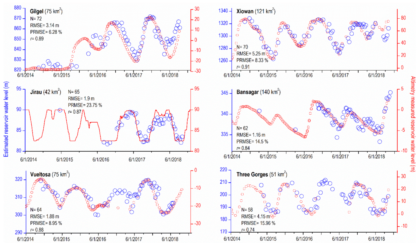
3.1. General Performance of the Proposed Approach

Comparison of our vegetation height rasters with the published global canopy data [44] yielded statistically significant relationships with high correlation coefficients over analyzed reservoirs (r ranging 0.64 to 0.83, Figure 3). A slight disagreement may relate to the three possible limitations of the data source. Simard et al. (2011) used to estimate the tree canopy at a global scale. First, the relatively coarse resolution (1 km) of the reference dataset does not account for subpixel variability in tree heights, which somewhat limits the local scale prediction. A second possible source of error could be the temporal gap between data collection, which is about 5 years. The canopy height was estimated using the Geoscience Laser Altimeter System (GLAS) aboard ICESat was collected in 2005, while SRTM data was collected in 2000. However, we verified with archive satellite imagery that there were no major land cover changes such as deforestation around the reservoirs we analyzed. Lastly, there is regional variability in the data quality due to the heterogeneous GLAS shot density that generally correlates with the accuracy of the tree height (Figure 3). Jirau was an exception that showed the lowest r value (0.64) among study sites, perhaps due to the dense canopy of the Amazon rainforest.
In this case, we present the results for WL estimation from 2014 to 2018 on six relatively recently built dams in five countries (Table 1, Figure 4). Our model accurately characterized WL dynamics and had relatively high correlation coefficient values between estimated and measured (e.g. altimetry) WL, which ranged from 0.74 to 0.91 (Figure 4). Since SRTM and MERIT DEM accuracy varies across areas with distinct vegetation cover and relief [41,45], we chose reservoirs in distinct geomorphological settings such as Jirau in the Amazon (<200 m above mean sea level) and Xiaowan in rugged Southwest China (>1000 m) to assess the method’s performance in different settings. WL estimated based on Sentinel–1 and SRTM data captured the seasonal variations and associated dam operational patterns of each reservoir with reasonable accuracy. The seasonal variation, including rising, falling, peak, and lowest WL is successfully demonstrated because Sentinel–1 image acquisition is not interrupted by atmospheric conditions or day–time. Calculated RMSE ranged from 1.16 to 5.25 m, with no seasonal variability of RMSEs in any of the studied reservoirs. We did not observe a difference in performance between high and low water seasons despite the height of the lake water surface and local hillslope encompassing the reservoir changes substantially between these two periods.
Low WL variation between peak and minimum WL was measured for broad lakes such as Bansagar (8 m, Son River Valley), Jirau (8 m, Amazon lowlands), and Vueltosa (21 m, Andean foothills) (Table 1). Reservoirs on steep valleys such as Gilgel (40 m calculated after stabilization in 2016, Omo–Gibe River Basin) and Xiaowan (63 m, Yunnan–Guizhou Plateau) had higher water level variation. To control for this large WL range in variability, we also considered percentage RMSE (pRMSE) of each reservoir to assess model performance. We contend that using pRMSE makes more sense than direct comparison using RMSE because the error range tends to increase as the WL variability increases and enables comparisons between reservoirs in different settings (Table 1). Half of the investigated reservoirs had pRMSE values < 10% (i.e. the uncertainty range is less than 10% of the total WL variability observed from 2014–2018). Gilgel and Xiowan reservoirs had the lowest pRMSE despite their high total WL variability.
While the model performed reasonably well for all reservoirs, Bansagar and Three Gorges had a pRMSE of ~15% and Jirau had a pRMSE of ~24%. Although Jirau presented the lowest WL variability (due to the nature of its run–of–river dam) and the tree height is estimated with the regression procedure using the densest GLAS shot (Figure 3), it had the highest pRMSE value of 24%. The relatively high error in Jirau might be due to substantial flooded forests upstream of the dam [47], which causes underestimation of WL during the flood season. Much of the land cover upstream of the Jirau Dam area in 2008 (pre–dam construction) was forest flooded by the reservoir. Since the SAR data we used (C–band) measures the backscatter of the tree canopy, the lake extent mapped in this case is likely smaller than the actual extent due to the flooded forest. Trees in this region are roughly 35 m in height on average [44], which is much larger than the WL variability of the reservoir. An aerial photograph taken in June 2014 (post–dam construction) shows a typical flooded forest during the flood season along the reservoir (Figure 5A). The effect of the flooded forest on increased error is shown by the consistent underestimation of WL using our method during the flood season in both 2017 and 2018 (Figure 4 and Figure 6A).
The higher uncertainty in WL at Three Gorges (15% pRMSE) could be explained by the three major issues. First, the Jason–2 altimetry pass is about 60 km upstream of the Three Gorges dam, while, in the other cases, altimetry passes within a few kilometers from the reservoir at the dammed site. Second, the seasonal dynamics of the reservoir’s water surface slope is also relatively higher than the other reservoirs, which may introduce additional discrepancies between altimetry and Sentinel–1 WL. There appears to be a general increase in RMSE when the water surface slope is sufficiently large (R2 = 0.91 when plotted the two variables over six reservoirs) (Table 1). Lastly, the GLAS shot density is relatively low in this area without reference data for validation, which might have underestimated the tree canopy height. The Bansagar reservoir presents a peculiar characteristic of rapid rise of WL and slow outflow. The rapid WL rise is likely related to the high rainfall rates during the monsoon season (July–September, see Figure S3). On the other hand, the reservoir presents the largest submerged area among the studies cases. Thus, we consider that these cases with relatively higher pRMSE are not attributed to the model’s performance but related to the availability of data and natural characteristics of the reservoir water surface. These issues may be overcome by using higher resolution or alternative data such as site–specific knowledge, such as the density of reference data, forest structures, or regional climatic conditions.
Although some possible sources of errors in this study are discussed above, a large enough sample size along the shoreline (N>>1000) should help mitigate errors somewhat by taking means (for WL) of a normally distributed curve (Figure 1). Residuals of estimated WL also do not present a clear trend depending on the number of points along the shoreline (Figure 5A). In fact, since all our investigated reservoirs had N>>1000 and yielded WL estimates with reasonable accuracy, we speculate that additional points along the reservoir shoreline would make the probabilistic mean even more robust.
We also investigated the effect of the reservoir elevation on the model’s accuracy. To tackle this issue, we analyzed the relationship between residuals (thus RMSEs) and the reservoir elevation. There was no statistically significant relation for all cases (Figure 5B). We suggest that there are two factors of this observation that offset each other. First, as the reservoirs expand during the wet season, their perimeters generally increase (although not for all cases, which depends on the valley geomorphology accommodating reservoirs), (Figure 6A).which raises the available shoreline points. However, during this season, the slope at the reservoir shoreline becomes steeper so the subpixel variations when extracting elevation values from the DEM is larger. Nevertheless, we acknowledge that the level of residuals depending on the number of shoreline points and the elevation could be further investigated with a larger number of case studies.
Although some remote sensing uncertainties discussed above might slightly lower the model’s accuracy, the critical advantage of our approach is the relatively consistent temporal coverage of estimated WL. This capability may solve problems such as the voids in altimetry data over the high–water season during 2016–2017 at the Three Gorges reservoir. Our model successfully estimated the rising and falling limbs of the WL for the missing period, estimating a peak WL of 212 m, which is a value close to adjacent years. Similar problems occurred for Vueltosa reservoir altimetry data during the high–water season of 2016–2017. Although more frequent in–situ measurement of WL might exist for hydroelectric reservoirs, they are often not readily available to the public. Thus, the proposed method could be a critical alternative to obtain WL series because it can fill the temporal gaps of altimetry data or the absence of gauged WL around the world.

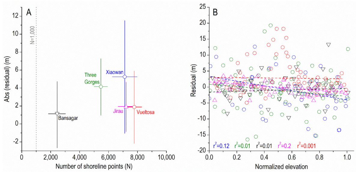
3.2. Effect of Local Slope over Different Elevation Ranges

Our results showed no significant effect of water surface elevation on RMSE, indicating that WL estimation accuracy is not dependent on seasonal variability. However, the standard deviation (STD) of the histograms used to derive the estimated WL for each date showed an increasing trend when plotted against normalized reservoir elevation (Figure 7).
( E l e v E l e v m i n E l e v m a x E l e v m i n )
Although WL accuracy did not appear to be related to reservoir elevation or season, uncertainty values increase with elevation. This pattern was observed for all investigated reservoirs except for Gilgel. We suspect that this pattern is related to local hillslope morphology because hillslope relief generally increases with altitude (assuming a concave longitudinal basin profile). Higher local hillslope relief translates to higher elevation changes for a given horizontal distance, and, therefore, STD (which indicates elevation variability) tends to increase. Gilgel reservoir had the only negative relationship between STD and water surface elevation as well as between elevation and slope. Topographic profiles of the Gilgel reservoir, drawn perpendicular to the river at the altimetry location, revealed that the valley confining the Gilgel reservoir is slightly convex as opposed to the typical concave shape of most profiles (Figure 6B).
It is difficult to provide a thorough analysis of the limitations that high slopes and small lakes have on the ability of this method to estimate WL. Practitioners adopting this (or similar methodology) should be aware of the potential limiting factors of slope and area, and determine what level of accuracy is necessary for their goals.

4. Discussion

Our proposed method based solely on remotely–sensed data is suitable to map most of the lakes and reservoirs worldwide (with the exception of some polar regions that lack SRTM coverage) without the need of in–situ instrumental analysis. The approach is conceptually simple and relatively easy to perform, so its adoption might benefit those with limited experience in remote sensing. We have provided a fully automated model to encourage others to use the proposed method for their own applications (Figure S1). Even with errors inherent in using the SRTM–derived DEMs, half of the case studies showed less than 10% pRMSE and, thus, should be considered a valid alternative to more complicated or more costly methods. In some reservoirs, data is lacking. Therefore, providing an initial estimate will also be valuable. Yet, we emphasize that practitioners adopting this method assess its validity against reference data (if possible).
The results are statistically robust due to the large number of points with extracted elevations distributed along the reservoir shoreline. Additionally, our method can be used to directly monitor WL changes with relatively high temporal resolution, providing estimates every 3 to 12 days depending on the local imaging plan of the Sentinel–1A and 1B satellites. One limitation of our method is that, for lakes or older reservoirs, which had high water levels during the SRTM mission flight (February 2000), an alternative DEM is needed to fill in the missing elevations inside the reservoir. In addition, the MERIT DEM, which is considered the most accurate bare–Earth DEM at a global scale still has limitations in high–slope regions where subpixel topographic variation is larger due to relatively coarse resolution [41]. Reservoirs that become ice–covered in the winter may result in seasonally larger uncertainties due to the ability of roughened ice to enhance the radar backscatter.
Previous studies have shown a good correlation between altimetry and ground truth data, normally ranging from a few centimeters for large lakes to a few decimeters for narrow reservoirs or rivers [48,49,50]. The coverage of these data is sparse due to a long distance between orbital tracks, and many reservoirs and lakes are still not surveyed. Although researchers have attempted to address the lack of altimetry data from below–nadir missions by using multi–mission approaches [51,52,53,54], nearly global coverage and regular gauging of reservoirs and lakes have not yet been attained.
Altimetry best measures WL at relatively large lakes and reservoirs (although there is no prescribed minimum size) because the observations are easily contaminated by backscatter from other ground reflectants. While we emphasize that accuracy of the method should be considered in terms of the project goals, we suggest that a minimum of 100 undisrupted (by atmospheric/terrain effects) shoreline points from the DEM layer, which fully encompasses a lake with a 3-km perimeter, should generally produce a normally distributed histogram to produce a robust WL. For some reservoirs, even a rough estimate of WL is a substantial improvement over the current lack of data. More than 99% of all existing lakes globally have a perimeter larger than 3 km [55], which means this method should be valid in the context of global proliferation of small dams [56].
The approach has valuable applications for investigating water dynamics in reservoirs, especially in the tropical and subtropical zones, where cloud–free optical images are often not available. By using the model developed in this study, the reservoir volume for certain WLs can be estimated. The models can be implemented from the construction of log (Area)–log (WL) and log(Volume)−log(Area) relationships for each impounded reservoir [57]. As the shoreline for each reservoir is delineated at every WL based on SAR images, the log−log relationships can be determined. The relationships can then be revised to power formulas, which indicates the area–volume relation (V = k * Aa) or the WL–volume relation (V = k * WLa) for the specific impoundment, where k and a are constants [58]. Using the formulas, the water storage fluctuation in reservoirs over a specific period can be calculated and could be used to investigate regional water resources availability.
Some studies have used optical satellite imagery combined with altimetry data to calculate reservoir storage variations [55,59,60]. This approach can be useful due to both the vast options of available optical satellite images in different levels of spatial resolutions and the long historical archive. The Landsat series started collecting data in the 1970s. However, optical images are daylight-dependent and subject to interference from cloud coverage, which are issues not pertinent to the active microwave sensor used to obtain Sentinel–1 SAR images. The backscattering images also have high contrast between land and water, which makes them ideal for the study of water bodies.
Our proposed method can also leverage emerging technologies like Unoccupied Aerial Vehicles (UAVs). The use of UAVs in geoscience has become ubiquitous [61], and allows for extremely accurate topographic measurements and DEMs that could be used with our proposed method. Recent advances in water surface elevation measurements in small inland water bodies show promise in potentially gauging rivers and small lakes [62,63], but larger lakes are more challenging and time–consuming to monitor with small UAVs. Therefore, it is important that WL monitoring methods have flexible data source inputs, and could integrate smaller–scale, high–resolution DEMs with satellite–based water masks.
Although a similar approach of overlaying lake extent with DEM to estimate elevation has been previously used, these were tested only in arid environments [35,36] or used airborne LiDAR–derived DEMs [37,38,39], which restricts the spatial coverage of the application. In addition, although the upcoming Surface Water Ocean Topography (SWOT) mission will substantially improve global inland water gauging [64], these data will not be collected until after 2022. Our proposed method, thus, considerably extends the current availability of global gauging data, which is crucial in a rapidly changing climate [2,65].

5. Conclusions

The continuous monitoring of all reservoirs and lakes over global scales has not yet been achieved but is critical for better understanding of the global hydrologic system. Issues of water scarcity, extreme and unpredictable flooding, the relationship between physical habitat and water availability, and the global increase in demand for hydroelectric power are all magnified in a changing climate. As humans are forced to adapt to changes in climate and the global hydrologic system, while many nations rapidly industrialize, the lack of consistently accurate measurements of reservoirs globally will put increasing strain on the Earth’s water resources.
We developed and verified a method of water level estimation using a combination of Sentinel–1 Synthetic Aperture Radar (SAR) observations and Shuttle Radar Topography Mission (SRTM) surface models, which produces water level estimates with high temporal resolution over global scales. While sensors and methods that rely on radar altimetry are more accurate, our method can monitor water bodies that are not directly located at the satellite’s nadir and water bodies substantially smaller in area. SAR data penetrates cloud cover, which is an improvement over optical methods, given that many reservoirs have recently been built in tropical, rain–rich and cloud–rich regions.
Our method is reasonably accurate compared to reference remotely–sensed and ground–based water surface elevation measurements in six reservoirs with distinct sizes, climates, and geomorphological settings. The proposed method is relatively simple to use and appears to be statistically robust despite a relationship between lake elevation and increased RMSE. Adoption of this or other similar SAR–based methods by environmental managers could be made easier by the proposed methodological guidelines (Figure S1) and easily accessible data used in this study. This study moves toward the true nearly–global gauging of reservoirs by providing water level estimates solely using operational remotely sensed data.

Supplementary Materials

The following are available online at https://www.mdpi.com/2072-4292/12/8/1353/s1. Figure S1: ArcGIS model builder developed to extract water level from Sentinel–A and SRTM DEM. Figure S2: Site map of the studied reservoir. Figure S3: Climograph processed from the Google Earth Engine over the Bansagar reservoir.

Author Contributions

Conceptualization, E.P. and E.M. Methodology, E.P., E.M., Q.W.L. and E.O.L. Analysis, E.P., E.M. and E.O.L. Writing—original draft preparation, E.P., E.M., Q.W.L. and E.O.L. Writing—review and editing, E.P., E.M., E.O.L., Q.W.L. and X.Y. funding acquisition, E.P. All authors have read and agreed to the published version of the manuscript.

Funding

The National Institute of Education (NIE) at Nanyang Technological University (NTU) Grant # SUG–NAP (3/19 EP) funded this research.

Acknowledgments

We acknowledge the USDA/NASA G–REALM program for making their altimetry product available through their website. Radar imagery used in this study are freely available Copernicus Sentinel data retrieved from the Alaska Satellite Facility (ASF) Distributed Active Archive Center (DAAC), processed by the European Space Agency (ESA). E.R.M. and Q.W.L. would like to thank São Paulo Research Foundation (FAPESP 2017/26318–8; 2016/14227–5) and the Environmental Resilience Institute funded by Indiana University’s Prepared for Environmental Change Grand Challenge initiative, respectively, for support during the development and writing of this manuscript.

Conflicts of Interest

The authors declare no conflict of interest.

References

  1. Vörösmarty, C.I.; Meybeck, M.-H.; Fekete, B.M.; Sharma, K.; Green, P.; Syvitski, J. Anthropogenic sediment retention: Major global impact from registered river impoundments. Glob. Planet. Chang. 2003, 39, 169–190. [Google Scholar] [CrossRef]
  2. Zarfl, C.; Lumsdon, A.E.; Berlekamp, J.; Tydecks, L.; Tockner, K. A global boom in hydropower dam construction. Aquat. Sci. 2015, 77, 161–170. [Google Scholar] [CrossRef]
  3. Winemiller, K.O.; Mcintyre, P.B.; Castello, L.; Fluet-Chouinard, E.; Giarrizzo, T.; Nam, S.; Baird, I.G.; Darwall, W.; Lujan, N.K.; Harrison, I.; et al. Balancing hydropower and biodiversity in the Amazon, Congo, and Mekong. Science 2016, 351, 128–129. [Google Scholar] [CrossRef] [PubMed] [Green Version]
  4. Latrubesse, E.M.; Arima, E.Y.; Dunne, T.; Park, E.; Baker, V.R.; d’Horta, F.M.; Wight, C.; Wittmann, F.; Zuanon, J.; Baker, P.A.; et al. Damming the rivers of the Amazon Basin. Nature 2017, 546, 363–369. [Google Scholar] [CrossRef]
  5. Fearnside, P.M. Tropical dams: To build or not to build? Science 2016, 351, 456–457. [Google Scholar] [CrossRef]
  6. Biemans, H.; Haddeland, I.; Kabat, P.; Ludwig, F.; Hutjes, R.; Heinke, J.; Von Bloh, W.; Gerten, D. Impact of reservoirs on river discharge and irrigation water supply during the 20th century. Water Resour. Res. 2011, 47. [Google Scholar] [CrossRef] [Green Version]
  7. Rothausen, S.G.; Conway, D. Greenhouse–gas emissions from energy use in the water sector. Nat. Clim. Chang. 2011, 1, 210–219. [Google Scholar] [CrossRef]
  8. Grill, G.; Lehner, B.; Thieme, M.; Geenen, B.; Tickner, D.; Antonelli, F.; Babu, S.; Borrelli, P.; Cheng, L.; Crochetiere, H.; et al. Mapping the world’s free–flowing rivers. Nature 2019, 569, 215. [Google Scholar] [CrossRef]
  9. Bernardo, N.; do Carmo, A.; Park, E.; Alcântara, E. Retrieval of Suspended Particulate Matter in Inland Waters with Widely Differing Optical Properties Using a Semi–Analytical Scheme. Remote Sens. 2019, 11, 2283. [Google Scholar] [CrossRef] [Green Version]
  10. Syvitski, J.P.; Vörösmarty, C.J.; Kettner, A.J.; Green, P. Impact of humans on the flux of terrestrial sediment to the global coastal ocean. Science 2005, 308, 376–380. [Google Scholar] [CrossRef]
  11. Park, E.; Latrubesse, E.M. A geomorphological assessment of wash–load sediment fluxes and floodplain sediment sinks along the lower Amazon River. Geology 2019, 47, 403–406. [Google Scholar] [CrossRef] [Green Version]
  12. Yang, Z.S.; Wang, H.J.; Saito, Y.; Milliman, J.D.; Xu, K.; Qiao, S.; Shi, G. Dam impacts on the Changjiang (Yangtze) River sediment discharge to the sea: The past 55 years and after the Three Gorges Dam. Water Resour. Res. 2006, 42. [Google Scholar] [CrossRef]
  13. Kummu, M.; Lu, X.; Wang, J.J.; Varis, O. Basin–wide sediment trapping efficiency of emerging reservoirs along the Mekong. Geomorphology 2010, 119, 181–197. [Google Scholar] [CrossRef]
  14. Mekonnen, M.M.; Hoekstra, A.Y. Four billion people facing severe water scarcity. Sci. Adv. 2016, 2, e1500323. [Google Scholar] [CrossRef] [PubMed] [Green Version]
  15. Veldkamp, T.I.; Wada, Y.; Aerts, J.; Döll, P.; Gosling, S.N.; Liu, J.; Masaki, Y.; Oki, T.; Ostberg, S.; Pokhrel, Y.; et al. Water scarcity hotspots travel downstream due to human interventions in the 20th and 21st century. Nat. Commun. 2017, 8, 15697. [Google Scholar] [CrossRef] [PubMed]
  16. Khadem, M.; Rougé, C.; Harou, J.; Hansen, K.M.; Medellin-Azuara, J.; Lund, J. Estimating the economic value of inter-annual reservoir storage in water resource systems. Water Resour. Res. 2018, 54, 8890–8908. [Google Scholar] [CrossRef]
  17. FAO; WWC. Towards a Water and Food Secure Future, in Critical Perspective for Policy–Makers; W.W. COUNCIL: Marseille, France, 2015. [Google Scholar]
  18. Pekel, J.F.; Cottam, A.; Gorelick, N.; Belward, A.S. High–resolution mapping of global surface water and its long–term changes. Nature 2016, 540, 418–422. [Google Scholar] [CrossRef]
  19. Crétaux, J.F.; Abarca-del-Río, R.; Berge-Nguyen, M.; Arsen, A.; Drolon, V.; Clos, G.; Maisongrande, P. Lake volume monitoring from space. Surv. Geophys. 2016, 37, 269–305. [Google Scholar] [CrossRef] [Green Version]
  20. Balsamo, G.; Salgado, R.; Dutra, E.; Boussetta, S.; Stockdale, T.; Potes, M. On the contribution of lakes in predicting near–surface temperature in a global weather forecasting model. Tellus A Dyn. Meteorol. Oceanogr. 2012, 64, 15829. [Google Scholar] [CrossRef] [Green Version]
  21. Yang, X.; Lu, X.; Park, E.; Tarolli, P. Impacts of Climate Change on Lake Fluctuations in the Hindu Kush–Himalaya–Tibetan Plateau. Remote Sens. 2019, 11, 1082. [Google Scholar] [CrossRef] [Green Version]
  22. Duan, Z.; Bastiaanssen, W. Estimating water volume variations in lakes and reservoirs from four operational satellite altimetry databases and satellite imagery data. Remote Sens. Environ. 2013, 134, 403–416. [Google Scholar] [CrossRef]
  23. Gao, H.; Zhang, S.; Durand, M.; Lee, H. Satellite Remote Sensing of Lakes and Wetlands. Hydrologic Remote Sensing; CRC Press: Boca Raton, FL, USA, 2016; pp. 57–72. [Google Scholar]
  24. Alsdorf, D.E.; Rodriguez, E.; Lettenmaier, D.P. Measuring surface water from space. Rev. Geophys. 2007, 45. [Google Scholar] [CrossRef]
  25. Nguy-Robertson, A.; May, J.; Dartevelle, S.; Birkett, C.; Lucero, E.; Russo, T.; Griffin, S.; Miller, J.; Tetrault, R.; Zentner, M. Inferring elevation variation of lakes and reservoirs from areal extents: Calibrating with altimeter and in situ data. Remote Sens. Appl. Soc. Environ. 2018, 9, 116–125. [Google Scholar] [CrossRef]
  26. Raclot, D. Remote sensing of water levels on floodplains: A spatial approach guided by hydraulic functioning. Int. J. Remote Sens. 2006, 27, 2553–2574. [Google Scholar] [CrossRef]
  27. Hostache, R.; Lai, X.; Monnier, J.; Puech, C. Assimilation of spatially distributed water levels into a shallow–water flood model. Part II: Use of a remote sensing image of Mosel River. J. Hydrol. 2010, 390, 257–268. [Google Scholar] [CrossRef] [Green Version]
  28. Westerhoff, R.S.; Kleuskens, M.P.H.; Winsemius, H.C.; Huizinga, H.J.; Brakenridge, G.R.; Bishop, C. Automated global water mapping based on wide–swath orbital synthetic–aperture radar. Hydrol. Earth Syst. Sci. 2013, 17, 651–663. [Google Scholar] [CrossRef] [Green Version]
  29. Huang, W.; DeVries, B.; Huang, C.; Lang, M.W.; Jones, J.W.; Creed, I.F.; Carroll, M.L. Automated extraction of surface water extent from Sentinel–1 data. Remote Sens. 2018, 10, 797. [Google Scholar] [CrossRef] [Green Version]
  30. Martinis, S.; Kersten, J.; Twele, A. A fully automated TerraSAR–X based flood service. ISPRS J. Photogramm. Remote Sens. 2015, 104, 203–212. [Google Scholar] [CrossRef]
  31. Van Bemmelen, C.W.T.; Mann, M.; De Ridder, M.; Rutten, M.; Van De Giesen, N. Determining water reservoir characteristics with global elevation data. Geophys. Res. Lett. 2016, 43, 11–278. [Google Scholar] [CrossRef] [Green Version]
  32. Zhang, S.; Gao, H. A novel algorithm for monitoring reservoirs under all-weather conditions at a high temporal resolution through passive microwave remote sensing. Geophys. Res. Lett. 2016, 43, 8052–8059. [Google Scholar] [CrossRef]
  33. Sheffield, J.; Ferguson, C.R.; Troy, T.J.; Wood, E.F.; McCabe, M.F. Closing the terrestrial water budget from satellite remote sensing. Geophys. Res. Lett. 2009, 36. [Google Scholar] [CrossRef]
  34. Park, E.; Lewis, Q.W.; Sanwlani, N. Large lake gauging using fractional imagery. J. Environ. Manag. 2019, 231, 687–693. [Google Scholar] [CrossRef] [PubMed]
  35. Amitrano, D.; Martino, G.D.; Iodice, A.; Mitidieri, F.; Papa, M.N.; Riccio, D.; Ruello, G. Sentinel–1 for monitoring reservoirs: A performance analysis. Remote Sens. 2014, 6, 10676–10693. [Google Scholar] [CrossRef] [Green Version]
  36. Chipman, J.W. A Multisensor Approach to Satellite Monitoring of Trends in Lake Area, Water Level, and Volume. Remote Sens. 2019, 11, 158. [Google Scholar] [CrossRef] [Green Version]
  37. Giustarini, L.; Matgen, P.; Hostache, R.; Montanari, M.; Plaza Guingla, D.A.; Pauwels, V.; De Lannoy, G.; De Keyser, R.; Pfister, L.; Hoffmann, L.; et al. Assimilating SAR–derived water level data into a hydraulic model: A case study. Hydrol. Earth Syst. Sci. 2011, 15, 2349–2365. [Google Scholar] [CrossRef] [Green Version]
  38. Mason, D.; Schumann, G.; Neal, J.; García-Pintado, J.; Bates, P.D. Automatic near real–time selection of flood water levels from high resolution Synthetic Aperture Radar images for assimilation into hydraulic models: A case study. Remote Sens. Environ. 2012, 124, 705–716. [Google Scholar] [CrossRef] [Green Version]
  39. Schumann, G.; Hostache, R.; Puech, C.; Hoffmann, L.; Matgen, P.; Pappenberger, F.; Pfister, L. High–resolution 3–D flood information from radar imagery for flood hazard management. IEEE Trans. Geosci. Remote Sens. 2007, 45, 1715–1725. [Google Scholar] [CrossRef]
  40. Birkett, C.M.; Beckley, B. Investigating the performance of the Jason–2/OSTM radar altimeter over lakes and reservoirs. Mar. Geod. 2010, 33, 204–238. [Google Scholar] [CrossRef]
  41. Amazaki, D.; Ikeshima, D.; Tawatari, R.; Yamaguchi, T.; O’Loughlin, F.; Neal, J.C.; Sampson, C.C.; Kanae, S.; Bates, P.D. A high-accuracy map of global terrain elevations. Geophys. Res. Lett. 2017, 44, 5844–5853. [Google Scholar] [CrossRef] [Green Version]
  42. Jarvis, A.; Reuter, H.I.; Nelson, A.; Guevara, E. Hole–Filled SRTM for the Globe Version 4. 2008. Available online: http://srtm.csi.cgiar.org/ (accessed on 20 August 2019).
  43. Farr, T.G.; Rosen, P.A.; Caro, E.; Crippen, R.; Duren, R.; Hensley, S.; Kobrick, M.; Paller, M.; Rodriguez, E.; Roth, L.; et al. The shuttle radar topography mission. Rev. Geophys. 2007, 45. [Google Scholar] [CrossRef] [Green Version]
  44. Simard, M.; Pinto, N.; Fisher, J.B.; Baccini, A. Mapping forest canopy height globally with spaceborne lidar. J. Geophys. Res. Biogeosci. 2011, 116. [Google Scholar] [CrossRef]
  45. Rodriguez, E.; Morris, C.S.; Belz, J.E. A global assessment of the SRTM performance. Photogramm. Eng. Remote Sens. 2006, 72, 249–260. [Google Scholar] [CrossRef] [Green Version]
  46. Birkett, C.; Reynolds, C.; Beckley, B.; Doorn, B. From research to operations: The USDA global reservoir and lake monitor. In Coastal Altimetry; Springer: Berlin, Heidelberg, 2011; pp. 19–50. [Google Scholar]
  47. Hess, L.L.; Melack, J.M.; Novo, E.M.; Barbosa, C.C.; Gastil, M. Dual–season mapping of wetland inundation and vegetation for the central Amazon basin. Remote Sens. Environ. 2003, 87, 404–428. [Google Scholar] [CrossRef]
  48. Birkett, C. The contribution of TOPEX/POSEIDON to the global monitoring of climatically sensitive lakes. J. Geophys. Res. Oceans 1995, 100, 25179–25204. [Google Scholar] [CrossRef]
  49. Zhang, G.; Xie, H.; Kang, S.; Yi, D.; Ackley, S.F. Monitoring lake level changes on the Tibetan Plateau using ICESat altimetry data (2003–2009). Remote Sens. Environ. 2011, 115, 1733–1742. [Google Scholar] [CrossRef]
  50. Ricko, M.; Carton, J.A.; Birkett, C.M.; Crétaux, J.F. Intercomparison and validation of continental water level products derived from satellite radar altimetry. J. Appl. Remote Sens. 2012, 6, 061710. [Google Scholar] [CrossRef] [Green Version]
  51. Berry, P.A.M.; Garlick, J.D.; Mathers, E.L.; Freeman, J.A. Global inland water monitoring from multi-mission altimetry. Geophys. Res. Lett. 2005, 32. [Google Scholar] [CrossRef]
  52. Song, C.; Huang, B.; Ke, L. Modeling and analysis of lake water storage changes on the Tibetan Plateau using multi–mission satellite data. Remote Sens. Environ. 2013, 135, 25–35. [Google Scholar] [CrossRef]
  53. Tong, X.; Pan, H.; Xie, H.; Xu, X.; Li, F.; Chen, L.; Luo, X.; Liu, S.; Chen, P.; Jin, Y. Estimating water volume variations in Lake Victoria over the past 22 years using multi–mission altimetry and remotely sensed images. Remote Sens. Environ. 2016, 187, 400–413. [Google Scholar] [CrossRef]
  54. Pham, H.T.; Marshall, L.; Johnson, F.; Sharma, A. Deriving daily water levels from satellite altimetry and land surface temperature for sparsely gauged catchments: A case study for the Mekong River. Remote Sens. Environ. 2018, 212, 31–46. [Google Scholar] [CrossRef]
  55. Verpoorter, C.; Kutser, T.; Seekell, D.A.; Tranvik, L.J. A global inventory of lakes based on high-resolution satellite imagery. Geophys. Res. Lett. 2014, 41, 6396–6402. [Google Scholar] [CrossRef]
  56. Couto, T.B.; Olden, J.D. Global proliferation of small hydropower plants–science and policy. Front. Ecol. Environ. 2018, 16, 91–100. [Google Scholar] [CrossRef]
  57. Sawunyama, T.; Senzanje, A.; Mhizha, A. Estimation of small reservoir storage capacities in Limpopo River Basin using geographical information systems (GIS) and remotely sensed surface areas: Case of Mzingwane catchment. Phys. Chem. Earth Parts A/B/C 2006, 31, 935–943. [Google Scholar] [CrossRef]
  58. Rodrigues, L.; Liebe, J. Small reservoirs depth–area–volume relationships in Savannah Regions of Brazil and Ghana. Water Resour. Irrig. Manag. 2013, 1, 1–10. [Google Scholar]
  59. Gao, H.; Birkett, C.; Lettenmaier, D.P. Global monitoring of large reservoir storage from satellite remote sensing. Water Resour. Res. 2012, 48. [Google Scholar] [CrossRef] [Green Version]
  60. Tarpanelli, A.; Amarnath, G.; Brocca, L.; Massari, C.; Moramarco, T. Discharge estimation and forecasting by MODIS and altimetry data in Niger–Benue River. Remote Sens. Environ. 2017, 195, 96–106. [Google Scholar] [CrossRef]
  61. Lewis, Q.W.; Park, E. Volunteered Geographic Videos in Physical Geography: Data Mining from YouTube. Ann. Am. Assoc. Geogr. 2018, 108, 52–70. [Google Scholar] [CrossRef]
  62. Bandini, F.; Jakobsen, J.; Olesen, D.; Reyna-Gutierrez, J.A.; Bauer-Gottwein, P. Measuring water level in rivers and lakes from lightweight Unmanned Aerial Vehicles. J. Hydrol. 2017, 548, 237–250. [Google Scholar] [CrossRef] [Green Version]
  63. Bandini, F.; Sunding, T.P.; Linde, J.; Smith, O.; Jensen, I.K.; Köppl, C.J.; Butts, M.; Bauer-Gottwein, P. Unmanned Aerial System (UAS) observations of water surface elevation in a small stream: Comparison of radar altimetry, LIDAR and photogrammetry techniques. Remote Sens. Environ. 2020, 237, 111487. [Google Scholar] [CrossRef]
  64. Biancamaria, S.; Lettenmaier, D.P.; Pavelsky, T.M. The SWOT mission and its capabilities for land hydrology. Surv. Geophys. 2016, 37, 307–337. [Google Scholar] [CrossRef] [Green Version]
  65. Di Baldassarre, G.; Wanders, N.; AghaKouchak, A.; Kuil, L.; Rangecroft, S.; Veldkamp, T.I.; Garcia, M.; van Oel, P.R.; Breinl, K.; Van Loon, A.F. Water shortages worsened by reservoir effects. Nat. Sustain. 2018, 1, 617–622. [Google Scholar] [CrossRef]
Figure 1. Flowchart illustrating the details of the full methodological framework to retrieve reservoir water surface elevation using SAR and DEM data, and validation, developed in this study. Corresponding Method sections (2.1–2.4) are also labelled.
Remotesensing 12 01353 g001
Figure 2. Filtering and de–noising process developed in this study (using a portion of Bansagar reservoir on 25 October 2017). (A): SAR amplitude image contains brighter back–reflection pixels, topographic shadowing in land, and speckles. (B): Through a thresholding method, the initial water extent was generated and then underwent the majority filtering. Note that noises are significantly reduced. (C): Remaining noises are further removed by eliminating small polygon and polyline parts to generate a trimmed reservoir shoreline. This process is iterated over all the available SAR images across reservoirs studied in this paper. (D): The result is compared with the Landsat 8 Operational Land Imager (OLI, acquired on 26 October 2017) driven modified NDWI (normalized difference water index) and false color RGB (653) image. (E): The detailed procedure is provided in Section 2.1 and Figure S1.
Remotesensing 12 01353 g002
Figure 3. Comparison of vegetation height rasters over analysed reservoirs in this study with a global scale canopy dataset. Correlation coefficients r are reported in parenthesis. Density of GLAS shots (per degree) used for the tree regression procedure by Simard and Pinto [44] for each reservoir is also presented.
Remotesensing 12 01353 g003
Figure 4. Six reservoir water levels (WL) (June 2014–October 2018) estimated in this study (blue) compared to reference altimetry series (red). Altimetry baseline has been adjusted to match the SRTM baseline. RMSE and percentage RMSE (pRMSE) are provided. In the case of Jirau, in situ WL data from ANA was used for validation.
Remotesensing 12 01353 g004
Figure 5. (A) Absolute value of residuals plotted against the number of shoreline points. Mean (symbol) and standard deviation (whisker) are shown. (B) Residuals of SAR–driven WL calculated from the altimetry series for each reservoir. WL estimates after the reservoir filling were considered.
Remotesensing 12 01353 g005
Figure 6. (A) High resolution PlanetScope image on May 2018 showing the maximum seasonal flooded area over the Jirau reservoir. Dense forests are flooded along most of the fringes of the reservoir. Aerial photo taken in June 2014 at the location of the green star symbol in the map. (B): Sentinel–derived points shoreline points over the Gilgel reservoir on 5 October 2016 overlaid on the bare–Earth DEM used in this study. Two convex elevation profiles and corresponding slopes are shown (C,D).
Remotesensing 12 01353 g006
Figure 7. (AC): Standard deviation vs. normalized elevation showing positive relationships except for Gilgel reservoir.
Remotesensing 12 01353 g007
Table 1. List of reservoirs investigated in this study. See location map provided in Figure S2.
ReservoirsLocation (Altimetry Intersection)CountrySentinel–1 PathYear Started to FillSurface Slope (m/km) aWater Level Variation (m) bRMSE (m) cpRMSE (%) d
Gilgel Gibe7°20′25”N, 37°20′77”EEthiopia15220151.09403.146.28
Xiowan24°50′17”N, 100°9′49”EChina9920091.76635.258.33
Jirau9°17′25”S, 64°41′15”WBrazil1562008 e0.4681.923.75
Bansagar24°4′27”N, 80°59′41”E.India56, 92, 16520110.0981.1614.5
Vueltosa7°44′34”N, 71°30′58”WVenezuela4, 17120090.18211.888.95
Three Gorges30°49′31”N, 111°0′14”EChina111994 e0.96264.1515.96
a Reported values are calculated as water surface slope averaged over the investigated period (2014–2018). b Water level range after the reservoir filling calculated from altimetry data (2014–2018). c Altimetry series dated within one week of the Sentinel–1 data collection were used for calculation. d Calculated as RMSE/WL variations. e Year construction started.

