Abstract
Several factors influence the performance of land change simulation models. One potentially important factor is land category aggregation, which reduces the number of categories while having the potential to reduce also the size of apparent land change in the data. Our article compares how four methods to aggregate Corine Land Cover categories influence the size of land changes in various spatial extents and consequently influence the performance of 114 Cellular Automata-Markov simulation model runs. We calculated the reference change during the calibration interval, the reference change during the validation interval and the simulation change during the validation interval, along with five metrics of simulation performance, Figure of Merit and its four components: Misses, Hits, Wrong Hits and False Alarms. The Corine Standard Level 1 category aggregation reduced change more than any of the other aggregation methods. The model runs that used the Corine Standard Level 1 aggregation method tended to return lower sizes of changing areas and lower values of Misses, Hits, Wrong Hits and False Alarms, where Hits are correctly simulated changes. The behavior-based aggregation method maintained the most change while using fewer categories compared to the other aggregation methods. We recommend an aggregation method that maintains the size of the reference change during the calibration and validation intervals while reducing the number of categories, so the model uses the largest size of change while using fewer than the original number of categories.
1. Introduction
Land change modelling is a popular research topic with a broad variety of approaches for understanding and simulating the temporal changes among land categories. Land change modeling supports decision-making concerning land management by giving insight into land-change processes and providing future scenarios by simulating future land mosaic and structure [1,2,3]. Within the variety of land change modeling approaches, Cellular Automata (CA)—Markov modelling is a widely known technique for land use/land cover (LULC) change simulation by extrapolating changes in a LULC map based on previous states of LULC in the spatial extent.
Data derive from a wide variety of sources. Landsat is one of the most popular. Initially called ERTS, the Landsat mission was launched in the 1970s—thus, its long history makes it possible to perform long-term land change analysis [4,5]. Another popular dataset is the imagery of the Sentinel satellites. The combined use of Sentinel’s radar and optical data allows for land monitoring temporally, because Sentinel’s frequent revisit time makes it possible to produce maps of land change during short time intervals [6,7]. Classification of land change requires procedures depending on the data source, such as hyperspectral images [8,9] or Synthetic Aperture Radar data [10,11]. Researchers can apply ready-to-use LULC datasets, like the Corine Land Cover database available in European countries. In the Corine Land Cover database, multiple datasets are available describing the LULC status in different years (1990, 2000, 2006, 2012 and 2018), making it possible to use it as an input for either monitoring [12,13] or simulation and validation [14,15] of land changes.
Category aggregation is the procedure to merge categories to form fewer categories. Aggregation is an important factor in land change modelling because some LULC maps have too many categories to analyze coherently. The aggregation of LULC map categories affects whether a specific categorical transition is present or eliminated from the extent. Aggregation of two categories erases the change between those two categories. Pontius Jr and Malizia (2004) [16] gave five mathematical rules that dictate how aggregation can reduce the size of temporal change. Pontius Jr et al. (2018) found that smaller amounts of reference change during the validation interval are associated with lower accuracies of land change simulation models [17].
Hierarchical classification schemes organize detailed categories for various levels of aggregation into broader categories. One of them is Anderson’s classification scheme [18], which is a nested hierarchical system of LULC categories, where a greater Anderson level has more categories. According to Guttenberg (2002) [19], the origin of multidimensional land use classification is related to urban planning that arose in the middle of the twentieth century. This approach of classification provided an opportunity for project-specific classifications [20]. Many category schemes exist, but there is no uniformly used category scheme because each scheme has its purpose and each project has its purpose [21]. For instance, Africover was a land cover category database for Africa particularly, created by FAO [22]. There are examples of vegetation-specific classification systems as well [23,24,25]. These latter category schemes focused on engaging the character of various vegetation types, therefore they could not be applied for general LULC classification in an area where non-vegetation LULC classes occur. The LULC classification scheme of Anderson [18] and Corine Land Cover Program [26] had the purpose of characterizing land cover in general because they had to characterize large areas with an extremely diversified LULC, e.g., covering a Pan-European scale in the case of Corine. Our research considers methods that aggregate any type of LULC classes.
Our article examines (1) how four aggregation methods affect the size of changes in eight spatial extents and (2) how the simulation model performance varies with the aggregation methods. To the best of our knowledge, this problem has not been analyzed in the literature concerning land change simulation modeling. We analyzed the reference change during the calibration interval, the reference change during the validation interval and simulation change during the validation interval concerning the original categories and four aggregation methods. We also computed five metrics concerning the performance of a CA-Markov simulation model and evaluated the results with special attention to category aggregation. We draw conclusions concerning the application of various aggregation methods and their impact on simulation model performance.
The Materials and Methods section describes the dataset, aggregation methods, model features and statistical analysis. The Results section gives several figures to visualize the findings. The Discussion section states the practical importance of the results and provides insights concerning best practices in aggregating data before running a land change simulation model.
2. Materials and Methods
2.1. Dataset
The input data are the Corine Land Cover (CLC) dataset, which is a pan-European land cover database. The database covers 39 countries, comprising the European Environment Agency (EEA) member and cooperating countries, including the members of the European Union. The CLC program was initiated in 1985 and there have been five datasets released so far. The datasets characterize LULC based on images taken approximately 1–2 years before the release dates. We used CLC datasets for the years 2000, 2006 and 2012. The time interval between 2000 and 2006 was the calibration interval and the time interval between 2006 and 2012 was the validation interval for all the models we ran. The CLC has its own nomenclature with a maximum of 44 categories, and the nomenclature is consistent over the databases from different years, hence making the years comparable and helping to monitor the changes over time. The nomenclature consists of 3 hierarchical levels, which are called standard levels. Standard level 1 has fewer categories than standard level 2, which has fewer categories than standard level 3. The CLC change maps were also produced based on the comparison of the consecutive years, and CLC change layers had a smaller minimal mapping unit than CLC layers, resulting in a finer land change dataset. CLC and CLC change layers are freely available from https://land.copernicus.eu/pan-european/corine-land-cover.
2.2. Study Area Selection According to Model Requirements
We analyze eight spatial extents that we selected in part based on the quantity of changing areas according to CLC Change layers for 2000–2006 and 2006–2012. The 8 extents were located across Europe and the extents were named after the cities closest to their location (Figure 1).
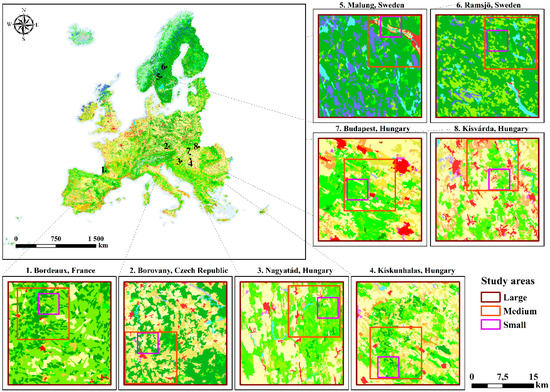
Figure 1.
Location of the analyzed landscapes, in the context of the complete CLC2012 data with a maximum of 44 categories. The locations are assigned with numbers to locate the study areas in the Pan-European Corine Land Cover (CLC) dataset. The smaller maps depict each study area by zoom level (large, medium and small) in the 8 landscapes.
We selected areas that had large sizes of changes during at least one of the time intervals of the analysis to test the model in various cases. Further conditions for selection were that the extents must have 20 categories as a maximum at each date and must have the same categories in at least the first two dates (2000 and 2006). The CA-Markov model cannot handle cases where a category at the end of the calibration interval does not exist at the beginning of the calibration interval. To each of the eight extents, we applied three zoom levels large (L), medium (M) and small (S). The large zoom level is identical to the extent. The medium zoom level is a subset of the large zoom level.
The small zoom level is a subset of the medium zoom level. The 24 combinations of the extent and zoom level were clipped from CLC’s 100 m resolution raster layers. The 24 selected combinations had the following characteristics:
- the areas had the same pixel number by zoom level (Large = 62,500 pixels; Medium = 15,625 pixels; Small = 2500 pixels);
- the areas had the same pixel resolution for all levels (100 m);
- the areas had the same categories in 2000 and 2006;
- the areas experienced as much change as possible according to the CLC change layers.
Then, in each of the 24 combinations of the extent and zoom level, we performed four category aggregation procedures. In 8 extents, 3 zoom levels and 5 aggregation methods we could have examined 120 models, but in six cases the aggregation did not make sense due to not meeting the condition of performing threshold-based aggregation, so we examined 114 models altogether.
2.3. Aggregation Methods
2.3.1. CLC Standard Levels
CLC database has a standard hierarchical nomenclature with 3 standard levels. The most detailed standard level is Level 3, which consists of 44 categories. The CLC dataset classifies land into these 44 categories based on various remotely-sensed data over time, processed along with matching a technical guideline [27]. Newer releases applied new remotely-sensed techniques [28]. Some processing methods varied over time, but all years have a uniform minimal mapping unit of 25 hectares, a thematic accuracy over 85% and a uniform nomenclature [26].
We used all three hierarchical levels of CLC datasets. We clipped our eight extents from the Level 3 dataset to maintain the same categories in 2000 and 2006, with a maximum of 20 categories in all combinations of extent and zoom. The CLC Level 3 (L3) classification has no category aggregation (Figure 2 and Figure 3).

Figure 2.
An example of category aggregation of CLC Level 3 categories according to the category aggregation schemes used in this research, based on study extent Borovany, Zoom level L (CLC L3 = categories according to CLC Level 3; L2 = categories according to CLC Level 2; L1 = categories according to CLC Level 1; BB = categories according to behavior-based category aggregation; TB = categories according to threshold-based category aggregation).
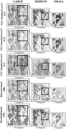
Figure 3.
Categories of a study area shown by zoom level in columns and aggregation methods in rows, assigned with the actual category numbers evolved as the result of aggregation. Shades of grey are not assigned to actual categories, but help to distinguish patches.
CLC Standard Level 2 consists of 15 categories as a maximum, where the 44 categories of Level 3 are aggregated into superior Level 2 categories. We aggregated the categories based on the CLC hierarchical nomenclature. We refer to this type of aggregation as CLC Level 2 (L2) aggregation (Figure 2 and Figure 3).
2.3.2. Behavior-Based Category Aggregation
The behavior-based category aggregation method originates from a research published by Aldwaik et al. (2015) [29], in which the authors presented a Microsoft Excel Visual Basic for Applications macro for a special type of category aggregation. This method aggregates categories based on the contingency table of the change between two dates. The behavior-based aggregation maintains net change, which is the change attributable to quantity differences of the categories between the two dates. The authors produced a free computer program that performs the aggregation for any transition matrix [29]. We used this computer program for executing the aggregation for the 24 combinations of extents and zoom levels. The program aggregates classes step by step, two categories in each step, while monitoring the total and net changes in each step. The user can follow if the total and net change starts to shrink in any of the steps. We aggregated the classes dictated by the behavior-based aggregation method in a manner that we stopped aggregating classes just before the total change started to decrease. In this way, the total change in the aggregated data equals the total change in the unaggregated data. We applied the algorithm for the calibration interval, then applied the same aggregation to the categories during the validation interval. We refer to this type of aggregation as behavior-based (BB) aggregation (Figure 2 and Figure 3).
2.3.3. Aggregation Based on Changes Observed in the Reference Intervals
The categories were aggregated based on the size of the change during the calibration and validation intervals. Based on a common threshold, we aggregated the categories that showed a total change of less than 0.1% of the actual extent in any of the calibration or validation intervals. This aggregation procedure was applied to the CLC Level 3 data, thus the unaggregated categories are identical to the CLC Level 3 categories. The categories not meeting the threshold were aggregated into a new category called Other. If there was no category meeting the threshold, then we did not perform any aggregation. That is why there are six cases of combination of the extent and zoom level where no aggregation was performed by this method. We refer to this type of aggregation as threshold-based (TB) aggregation (Figure 2 and Figure 3).
Figure 2 shows how detailed categories are aggregated to fewer broader categories for a specific combination of extent and zoom, according to the rules of each aggregation method. CLC Standard Level 3 consists of the 13 categories that occurred in Borovany extent, Zoom Level L according to Level 3 categories. The CLC Standard system is a hierarchical category scheme, so the categories of the more detailed CLC Standard Level 3 are aggregated into broader Standard 2 (L2) categories and broader Standard 2 (L2) categories.
The BB category aggregation method resulted in two of the original classes and three aggregated classes. The BB method considers the change characteristics during the calibration interval in the combination of study extent and zoom. BB may aggregate categories that are thematically diverse. For example, Figure 2 shows Discontinuous urban fabric aggregated with Transitional woodland-scrub. The BB algorithm maintains change by aggregating categories that do not transition with each other.
TB aggregation also resulted in six original categories and one category called Other. This Other category is the aggregation of seven thematically diverse categories. These categories account for extremely small changes. Consequently, the land change model focuses on the categories that provide relatively larger changes in the landscape.
2.4. CA-Markov Model
For the 114 cases (Table 1), we applied a Cellular Automata–Markov (CA-Markov) model in Idrisi Selva software [30]. This model is based on two components. First, a Markov matrix characterizes the categorical transitions from 2000 to 2006, then extrapolates the number of pixels of each transition from 2006 to 2012. The Markov matrix determines the number of pixels that transition from each category to every other category during the extrapolated time interval [31,32]. Second, the CA-algorithm influences the spatial allocation of extrapolated change from 2006 to 2012 based on the default settings in Idrisi’s algorithm concerning neighboring pixels [33,34].

Table 1.
A matrix of extents and aggregation methods concerning how we ran our models. Aggregation methods are named according to Section 2.3. L, M and S letters are abbreviations for Large, Medium and Small zoom levels, referring to their area size. Positive (+) signs denote that model was run in the relevant extent, zoom level and aggregation method according to their positions in the matrix. Negative (–) signs denote that model was not run for that specific case.
In our models, along with CLC database contents, 2000, 2006 and 2012 land cover maps determined reference time 1, reference time 2 and reference time 3, respectively. The changes between 2000 and 2006 are the calibration interval changes. The changes between 2006 and 2012 are the validation interval changes, based on which the model was validated. The CA-Markov model simulated land cover changes from 2006 to 2012. Then we compared the reference changes to the simulation changes during 2006–2012. All the models were run with an iteration number of 6 and a 5 × 5 contiguity filter. By using the same parameters, we ensured that the various model parameters did not influence the investigation of the factors playing an important role in model validation or performance.
2.5. Metrics Concerning Calibration and Validation Intervals
All the model runs derived from the 8 extents, 3 zoom levels and 5 aggregation methods. Before running the models, we measured the following:
- the changing areas in the calibration interval as a percentage of the actual combination of the extent and zoom level;
- the changing areas in the validation interval as a percentage of the actual combination of the extent and zoom level;
- the number of categories in reference time 1, reference time 2 and reference time 3 maps.
The figure of merit (FOM) is a measurement especially used for simulation models, describing the match of predicted and observed change [17,35,36]. If the FOM is 0%, then there is no intersection of predicted and observed change. If the FOM is 100%, then there is a complete overlap between predicted and observed change. The FOM components provide a deeper insight into the similarity of changes [37]. The FOM components show all types of incorrectly and correctly predicted change as a percentage of the size of the combination of the extent and zoom level, as follows:
Misses = area of observed change predicted as persistence (incorrect);
Hits = area of observed change predicted as change to the correct category (correct);
Wrong Hits = area of observed change predicted as change to the wrong category (incorrect);
False Alarms = area of observed persistence predicted as change (incorrect) [17].
We calculated for all the 114 model runs the FOM and its components: Misses, Hits, Wrong Hits, and False Alarms. These metrics were calculated in R software [38] with the ‘lulcc’ package [39].
2.6. Statistical Analysis
According to the Shapiro-Wilk test, the distribution of the metrics did not follow the normal distribution, therefore, we applied robust Two-Way factorial ANOVA to reveal the effects of aggregation and the study sites in the specific measures of calibration, validation and simulation changes, FOM and its components. We applied bootstrapping with 599 repetitions and the median as the estimator. Our Null Hypothesis was that (i) the medians of the four aggregation methods and the original data were equal, (ii) the medians of eight study sites were equal and (iii) there was no statistical interaction between these factors (i.e., the effects of aggregation do not depend on the study sites) [40,41]. When robust ANOVA test statistics were not available with the bootstrap design, we reported only the p-values. Results of post hoc analysis were plotted in boxplot diagrams focusing on the aggregation methods, significant differences (p < 0.05) were signed with different letters in the upper section of the diagrams, i.e., groups that are significantly different from each other had different letters, while the groups with indistinguishable medians had an identical letter above the boxplots [42].
Statistical analysis was conducted in R software [38] using ‘ggplot2′ [43], WRS2 [44]. We also used the jamovi 1.2. software [45].
3. Results
The number of categories was different by the aggregation methods: L1 aggregation method had the fewest number of categories, BB and L2 aggregation methods had fewer categories relative to L3 and TB in general.
L1, L2 and L3 groups had a theoretical maximum of 5, 15 and 44 categories, respectively because those are the number of categories at each level in the Corine data. Our data had a maximum of 5, 12 and 18 categories, respectively. The cases aggregated by BB and TB aggregation methods had a theoretical maximum of 44 categories, as they derived from L3 data, but the BB and TB aggregations were based on the sizes and types of change. BB and TB aggregation methods had a maximum of 9 and 13 categories, respectively (Figure 4).
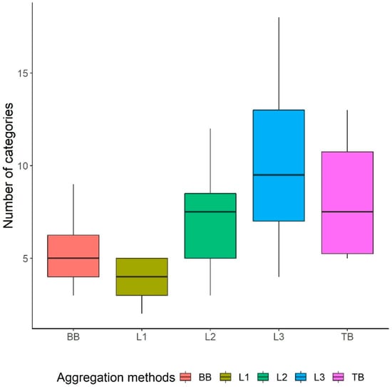
Figure 4.
Number of categories in the calibration interval in the whole dataset by aggregation method (BB = Behavior-based aggregation; L1 = Corine Standard Level 1 aggregation; L2 = Corine Standard Level 2 aggregation; L3 = Corine Standard Level 3 aggregation; TB = Threshold-based aggregation). BB, L1, L2, L3 and TB groups include 24,24,24,24 and 18 model runs, respectively. The vertical middle line shows the median, the box boundaries show the first and third quartiles of the method, the lower and upper end of whiskers show the minimum and maximum values of the method.
We analyzed the changes as a percent of the study area for the calibration (2000 reference–2006 reference), validation (2006 reference–2012 reference) and simulation (2006 reference–2012 simulation) intervals grouped by aggregation methods. The differences among medians of the groups were significant (Table 2), meaning we reject the hypothesis that all medians are identical. According to the post hoc analysis, the median change in the L1 group was significantly less than the median of the other aggregation methods in either calibration, validation or simulation intervals (Figure 5).
Table 2.
Factorial ANOVA results of the percent of changes in the calibration, validation and simulation intervals by aggregation methods (H0: medians of calibration intervals, validation intervals and simulation intervals are equal).
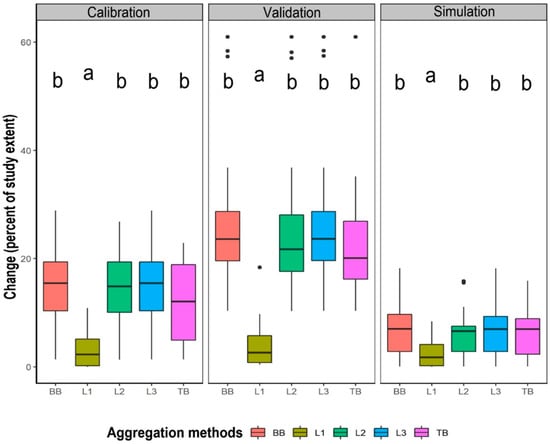
Figure 5.
Changes in the study areas expressed as a percent of the study extent, grouped by aggregation method (A) reference change during 2000–2006 (B) reference change during 2006–2012 and (C) simulated change during 2006–2012. The groups for which the medians are not significantly different are assigned a common letter. (BB = Behavior-based aggregation; L1 = Corine Standard Level 1 aggregation; L2 = Corine Standard Level 2 aggregation; L3 = Corine Standard Level 3 aggregation). BB, L1, L2, L3 and TB groups include 24,24,24,24 and 18 model runs, respectively. The vertical middle line shows the median, the box boundaries show the first and third quartiles of the group, the lower and upper end of whiskers show the minimum and maximum values that are not outliers, while the points show the outliers.
Figure 6 shows that the aggregation methods had an insignificant effect on the FOM median. L1 had a slightly wider range of FOM values, TB had a slightly tighter range of FOM values related to groups of BB, L2 and L3 groups. However, Figure 6 showed that the median of L1 was less than the median of other aggregation methods. However, effect sizes indicated a larger effect regarding the magnitude of differences between L1 and other aggregation techniques (L1-BB: 0.30, L1-L2: 0.29, L1-L3: 0.31, L1-TB: 0.30). In comparison, the largest difference of other aggregation techniques was between L2 and L3, the effect size was 0.002, indicating smaller effect.
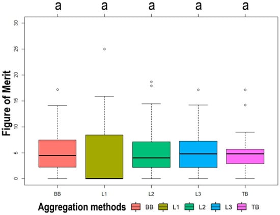
Figure 6.
Figure of Merit (FOM) values grouped by the aggregation method. No groups are significantly different, therefore the single letter a at the top applies to all groups. (BB = Behavior-based aggregation; L1 = Corine Standard Level 1 aggregation; L2 = Corine Standard Level 2 aggregation; L3 = Corine Standard Level 3 aggregation). BB, L1, L2, L3 and TB groups include 24,24,24,24 and 18 model runs, respectively. The vertical middle line shows the median, the box boundaries show the first and third quartiles of the group, whiskers show the minimum and maximum values that are not outliers, while points show the outliers.
Components of Figure of Merit (FOM)—Wrong Hits, False Alarms, Misses and Hits—by aggregation methods had significant differences on the medians (Table 3). Wrong Hits, False Alarms and Misses showed different types of disagreement between reference and simulated changes (Figure 7). All of these components were lower for L1 relative to the other aggregation methods. Hits are the agreement between reference and simulated changes. Hits were also lower for L1 relative to the other aggregation methods. Hits and Wrong Hits in the L1 group were significantly different from L2, L3 and BB groups. False alarms in the L1 group were significantly different from L3 and BB groups. Misses in the L1 group were significantly different from groups of all the other aggregation methods.
Table 3.
Result of the Kruskal-Wallis test of the Figure of Merit components by aggregation methods (H0: medians of FOM components are equal).
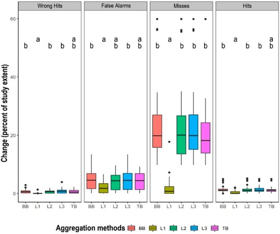
Figure 7.
Figure of Merit (FOM) components expressed as a percent of the study area, grouped by aggregation method, where Wrong Hits = area of observed change predicted as change to the wrong category, False Alarms = area of observed persistence predicted as change, Misses = area of observed change predicted as persistence, Hits = area of observed change predicted as change to the correct category. The groups that are not significantly different are assigned a common letter. BB, L1, L2, L3 and TB groups include 24,24,24,24 and 18 model runs, respectively. The vertical middle line shows the median, the box boundaries show the first and third quartiles of the group, the lower and upper end of whiskers show the group’s minimum and maximum values that are not outliers, while the points show the outliers.
4. Discussion
4.1. Effects of Changes in the Study Area
Based on the results of calibration, validation and simulation interval changes, the L1 group showed a lower ratio of changes in the study area, according to other groups, as Figure 4 depicts. The range of the ratio of changes in all other aggregation methods, excluding L1, was similar and they were not significantly different from each other. It means that L1 aggregation eliminates more change relative to the other aggregation methods, and all the other aggregation methods show a similar ratio of changes in the study areas. L1 aggregation results in a lower amount of changes in the study area, which makes sense because L1 has fewer categories. L1 aggregation rules are based on Corine’s thematic hierarchy [46].
Corine’s hierarchical structure dictates the L1 and L2 aggregations, regardless of the empirical patterns during any time interval. The LULC changes during the calibration interval guide the BB and TB aggregations. When detailed categories are aggregated, the model cannot simulate changes among those detailed categories during the validation interval, even when those detailed categories account for change during the validation interval.
4.2. Effects of FOM and FOM Components
Pontius Jr et al. 2008 [47] found that FOM tended to return larger values where reference maps had larger amounts of observed net change. In our case, the median FOM for the L1 group was not statistically significantly different from the other aggregation methods. However, the L1 group’s minimum FOM was equal to its median FOM, which was equal to 0. This highlights the limitations of hypothesis testing, which can be misleading, as several authors have concluded [48,49,50,51]. Here, differences among L1 and other aggregation methods were not significant, but half of L1′s FOM values were less than the lower quartiles for all other aggregations.
L1 values were generally lower in terms of Wrong Hits, False Alarms, Misses and Hits. All the other aggregation methods were similar in terms of Wrong Hits, False Alarms, Misses and Hits. The L1 group was significantly different from L2, L3 and BB groups in terms of Hits and Wrong Hits. The L1 group was significantly different from L3 and BB groups in terms of False Alarms. The L1 group was significantly different from groups of all the other aggregation methods in terms of Misses. These components are calculated based on changing areas by definition [17] and they are given as a percent of the study area. Due to this fact, while eliminating changes in the study area, the possibility of showing a higher value of any of the FOM components related to other aggregation methods becomes less possible in the case of L1. While L1 had fewer changing areas, it had lower values in terms of all FOM components related to other aggregation methods, in a statistically significant way or based on visual interpretation. Hits values mean the correctly simulated changes in the simulation map and the other three components determine the erroneously simulated changes. Since all examined components are lower in the case of the L1 group, it means a lower ratio of erroneously predicted areas, but means a lower ratio of correctly simulated changes simultaneously. It refers to the fact that the simulation model in the case of the L1 group explains less change. While the FOM is not enough to qualify model performance, as stated in Varga et al. 2019 [37], four FOM components—Wrong Hits, False Alarms, Misses and Hits—return lower values in L1 group, where lower ratios of observed changing areas were also present in either calibration or validation intervals. However, we do not know about any papers focusing on the statistical relationship between FOM components and observed changes.
4.3. Effects of Category Numbers
Although the aggregation methods, excluding L1, had similar characteristics concerning FOM components and ratios of change in the study areas, it is important to pay attention to the number of categories as well. Aldwaik et al. (2015) [29] stated that if maps have a larger number of categories, it may cause difficulties in the interpretation of the analysis. The behavior-based algorithm decreases the number of categories while maintaining change. BB, L2 and L3 were not significantly different in terms of Hits values, but the BB group had generally lower numbers of categories. It refers to the fact that while BB aggregation decreases the number of categories, it does not have lower Hits values related to other aggregation methods with a generally larger number of categories. The decrease of category numbers may result in an easier interpretation and a lower demand for computing resources when running a simulation model. Besides the lower number of categories, BB aggregation has also an advantage that the category aggregation rules aim to maintain changes in the area. Although L1 aggregation also results in a low number of categories, L1 aggregation eliminates changes in the area as described above. TB aggregation method is also based on maintaining some of the changing categories, but with an arbitrary threshold of changes in the area. TB aggregation did not make it possible to maintain the most changes possible, because the changes not meeting the arbitrary threshold were eliminated. Moreover, TB aggregation did not reduce the number of categories as much as BB and L1 aggregations. Consequently, we recommend an aggregation method that maintains changes and correctly simulated changing areas in the study area along with reducing the number of categories as much as possible. Based on the results, we recommend BB aggregation of all the applied aggregation methods as a best practice, instead of applying CLC standard level aggregation. CLC standard level aggregation matches a hierarchical system while eliminating changes in the study area and resulting in lower ratios of correctly and incorrectly simulated changing areas, therefore a lower ratio of explained changes. If we know the effect of category aggregation on model performance, then we will be able to eliminate a factor that may result in a less informative insight into the model performance.
5. Conclusions
Our paper describes an analysis concerning 114 runs of a CA-Markov simulation model, which were based on LULC maps derived from Corine Land Cover data and were generated with four aggregation methods. We analyzed the effects of aggregation methods on changes in the study areas, the Figure of Merit (FOM) and FOM’s components: Wrong Hits, False Alarms, Misses, Hits. We have five main conclusions. First, L1 and BB aggregations produced the fewest categories. Second, BB aggregation maintained the largest sizes of changes. Third, L1 had generally lower sizes of changes in the calibration, validation and simulation intervals. Fourth, L1 medians of change were considerably lower, specifically, half of the medians were zero. Fifth, L1 had generally lower values in terms of all FOM components. Based on the results and the aggregation rules of various aggregation methods, we warn users that the Corine standard level aggregation rules can eliminate sizeable changes. We recommend users apply aggregation methods that reduce the number of categories while maintaining changes and not reducing the correctly simulated changes in the area. In our analysis, the behavior-based aggregation method met these goals. We also recommend that users calculate FOM and FOM’s components to gain important insights concerning the interaction of the simulation model performance and changes in the reference data.
Author Contributions
Conceptualization, O.G.V. and R.G.P.J.; methodology, O.G.V., R.G.P.J., S.S.; software, O.G.V., S.S.; validation, S.S.; formal analysis, O.G.V. and S.S.; investigation, O.G.V.; resources, O.G.V.; data curation, O.G.V.; writing—original draft preparation, O.G.V.; writing—review and editing, O.G.V., R.G.P.J., S.S.; visualization, O.G.V.; supervision, S.S.; project administration, Z.S.; funding acquisition, Z.S. and S.S. All authors have read and agreed to the published version of the manuscript.
Funding
On behalf of Szilárd Szabó, this research was funded by the NKFI, with grant number TNN 123457.
Acknowledgments
The research was financed by the Thematic Excellence Programme of the Ministry for Innovation and Technology in Hungary (ED_18-1-2019-0028), within the framework of the Space Sciences thematic programme of the University of Debrecen.
Conflicts of Interest
The authors declare no conflict of interest. The funders had no role in the design of the study; in the collection, analyses, or interpretation of data; in the writing of the manuscript, or in the decision to publish the results.
References
- Brown, D.G.; Verburg, P.H.; Pontius Jr, R.G.; Lange, M.D. Opportunities to Improve Impact, Integration, and Evaluation of Land Change Models. Curr. Opin. Environ. Sustain. 2013, 5, 452–457. [Google Scholar] [CrossRef]
- Paegelow, M.; Camacho Olmedo, M.T.; Mas, J.; Houet, T.; Pontius Jr, R.G. Land Change Modelling: Moving Beyond Projections. Inter. J. Geogr. Inf. Sci. 2013, 27, 1691–1695. [Google Scholar] [CrossRef]
- Lundberg, A. Recent Methods, Sources and Approaches in the Study of Temporal Landscape Change at Different Scales—A Review. Hung. Geogr. Bull. 2018, 67, 309–318. [Google Scholar] [CrossRef]
- Ruelland, D.; Dezetter, A.; Puech, C.; Ardoin-Bardin, S. Long-Term Monitoring of Land Cover Changes Based on Landsat Imagery to Improve Hydrological Modelling in West Africa. Inter. J. Remote Sens. 2008, 29, 3533–3551. [Google Scholar] [CrossRef]
- Viana, C.M.; Girão, I.; Rocha, J. Long-Term Satellite Image Time-Series for Land use/Land Cover Change Detection using Refined Open Source Data in a Rural Region. Remote Sens. 2019, 11, 1104. [Google Scholar] [CrossRef]
- Szostak, M.; Hawryło, P.; Piela, D. Using of Sentinel-2 Images for Automation of the Forest Succession Detection. Eur. J. Remote Sens. 2018, 51, 142–149. [Google Scholar] [CrossRef]
- Tavares, P.A.; Beltrão, N.E.S.; Guimarães, U.S.; Teodoro, A.C. Integration of Sentinel-1 and Sentinel-2 for Classification and LULC Mapping in the Urban Area of Belém, Eastern Brazilian Amazon. Sensors 2019, 19, 1140. [Google Scholar] [CrossRef]
- Li, X.; Yuan, Z.; Wang, Q. Unsupervised Deep Noise Modeling for Hyperspectral Image Change Detection. Remote Sens. 2019, 11, 258. [Google Scholar] [CrossRef]
- Burai, P.; Deák, B.; Valkó, O.; Tomor, T. Classification of Herbaceous Vegetation using Airborne Hyperspectral Imagery. Remote Sens. 2015, 7, 2046–2066. [Google Scholar] [CrossRef]
- Deng, L.; Wang, H.H.; Li, D.; Su, Q. Two-Stage Visual Attention Model Guided SAR Image Change Detection. In Proceedings of the International Conference on Smart Systems and Inventive Technology (ICSSIT), Tamil Nadu, India, 27–29 November 2019. [Google Scholar]
- Coca, M.; Anghel, A.; Datcu, M. Unbiased Seamless SAR Image Change Detection Based on Normalized Compression Distance. IEEE J. Sel. Top. Appl. Earth Obs. Remote Sens. 2019, 12, 2088–2095. [Google Scholar] [CrossRef]
- Cieślak, I.; Szuniewicz, K.; Pawlewicz, K.; Czyża, S. Land use Changes Monitoring with CORINE Land Cover Data. In Proceedings of the IOP Conference Series Materials Science and Engineering, Prague, Czech Republic, 12–16 June 2017; p. 245. [Google Scholar]
- Yilmaz, R. Monitoring Land use/Land Cover Changes using CORINE Land Cover Data: A Case Study of Silivri Coastal Zone in Metropolitan Istanbul. Environ. Monit. Assess. 2010, 165, 603. [Google Scholar] [CrossRef]
- Dzieszko, P. Land-Cover Modelling using Corine Land Cover Data and Multilayer-Perceptron. Quaest. Geogr. 2015, 33, 5–22. [Google Scholar] [CrossRef]
- Viana, C.M.; Rocha, J. Land use Land Cover Changes in Beja District Based on the Markov and Cellular Automata Models. In Proceedings of the 11th International Conference of the Hellenic Geographical Society; Innovative Geographies: Understanding and Connecting our World, Lavrion, Greece, 12–15 April 2018. [Google Scholar]
- Pontius Jr, R.G.; Malizia, N.R. Effect of Category Aggregation on Map Comparison. In Geographic Information Science. GIScience 2004. Lecture Notes in Computer Science; Springer: Berlin/Heidelberg, Germany, 2004; pp. 251–268. [Google Scholar]
- Pontius Jr, R.G.; Castella, J.; De Nijs, T.; Duan, Z.; Fotsing, E.; Goldstein, N.; Kok, K.; Koomen, E.; Lippitt, C.D.; McConnell, W.; et al. Lessons and Challenges in Land Change Modeling Derived from Synthesis of Cross-Case Comparisons. In Trends in Spatial Analysis and Modelling, Geotechnologies and the Environment 19 ed.; Behnisch, M., Meine, G., Eds.; Springer International Publishing: Cham, Germany, 2018; pp. 143–164. [Google Scholar]
- Anderson, J.R.; Hardy, E.E.; Roach, J.T.; Witmer, E. A Land use and Land Cover Classification System for use with Remote Sensor Data; Geological Survey Professional Paper 964; US Government Printing Office: Washington, DC, USA, 1976.
- Guttenberg, A. Multidimensional Land use Classification and how it Evolved: Reflections on a Methodological Innovation in Urban Planning. J. Plan. Hist. 2002, 1, 311–324. [Google Scholar] [CrossRef]
- Bach, P.M.; Staalesen, S.; McCarthy, D.T.; Deletic, A. Revisiting Land use Classification and Spatial Aggregation for Modelling Integrated Urban Water Systems. Landsc. Urban Plan. 2015, 143, 43–55. [Google Scholar] [CrossRef]
- Di Gregorio, A.; Jansen, L.J.M. Land Cover Classification System (LCCS): Classification Concepts and User Manual; FAO, 2000. Available online: http://www.fao.org/3/x0596e/x0596e00.htm (accessed on 22 October 2019).
- Food and Agriculture Organization of the United Nations (FAO). AFRICOVER Land Cover Classification; FAO: Rome, Italy, 1997. [Google Scholar]
- Fosberg, F.R. A Classification of Vegetation for General Purposes. Trop. Ecol. 1961, 2, 1–28. [Google Scholar]
- Eiten, G. Vegetation Forms. A Classification of Stands of Vegetation Based on Structure, Growth Form of the Components, and Vegetative Periodicity; Boletim do Instituto de Botanica: San Paulo, Brazil, 1968. [Google Scholar]
- UNESCO. International Classification and Mapping of Vegetation; UNESCO: Paris, France, 1973. [Google Scholar]
- Büttner, G. CORINE Land Cover and Land Cover Change Products. In Land use and Land Cover Mapping in Europe; Manakos, I., Braun, M., Eds.; Springer: Dordrecht, The Netherlands, 2014; pp. 55–74. [Google Scholar]
- Büttner, G.; Feranec, J.; Jaffrain, G.; Mari, L.; Maucha, G.; Soukup, T. The CORINE Land Cover 2000 Project. EARSeL eProceedings 2004, 3, 331–346. [Google Scholar]
- Büttner, G.; Kosztra, B. CLC2018 Technical Guidelines. 2017. Available online: https://land.copernicus.eu/user-corner/technical-library/clc2018technicalguidelines_final.pdf (accessed on 22 October 2019).
- Aldwaik, S.Z.; Onsted, J.A.; Pontius Jr, R.G. Behavior-Based Aggregation of Land Categories for Temporal Change Analysis. Inter. J. Appl. Earth Obs. Geoinf. 2015, 35, 229–238. [Google Scholar] [CrossRef]
- Eastman, J.R. Idrisi Selva Geospatial Monitoring and Modeling System; Clark University: Worcester, MA, USA, 2012.
- Bruzzone, L.; Serpico, S.B. An Iterative Technique for the Detection of Land-Cover Transitions in Multitemporal Remote-Sensing Images. IEEE Trans. Geosci. Remote Sens. 1997, 35, 858–867. [Google Scholar] [CrossRef]
- Schweitzer, P.J. Perturbation Theory and Finite Markov Chains. J. Appl. Probab. 1968, 5, 401–413. [Google Scholar] [CrossRef]
- Baker, W. A Review of Models of Landscape Change. Landsc. Ecol. 1989, 2, 111–133. [Google Scholar] [CrossRef]
- Sipper, M. Evolving uniform and non-uniform cellular automata networks. In Annual Reviews of Computational Physics, 5th ed.; Stauffer, D., Ed.; World Scientific: Singapore, 1997; pp. 243–285. [Google Scholar]
- Klug, W.; Graziani, G.; Grippa, G.; Pierce, D.; Tassone, C. Evaluation of Long Range Atmospheric Transport Models using Environmental Radioactivity Data from the Chernobyl Accident: The ATMES Report; Springer Netherlands: Dordrecht, Netherlands, 1992. [Google Scholar]
- Perica, S.; Foufoula-Georgiou, E. Model for Multiscale Disaggregation of Spatial Rainfall Based on Coupling Meteorological and Scaling Descriptions. J. Geophys. Res.: Atmos. 1996, 101, 26347–26361. [Google Scholar] [CrossRef]
- Varga, O.G.; Pontius Jr, R.G.; Singh, S.K.; Szabó, S. Intensity Analysis and the Figure of Merit’s Components for Assessment of a Cellular Automata—Markov Simulation Model. Ecol. Indic. 2019, 101, 933–942. [Google Scholar] [CrossRef]
- R Core Team. A Language and Environment for Statistical Computing. 2019. Available online: https://www.eea.europa.eu/data-and-maps/indicators/oxygen-consuming-substances-in-rivers/r-development-core-team-2006 (accessed on 22 October 2019).
- Moulds, S.; Buytaert, W.; Mijic, A. An Open and Extensible Framework for Spatially Explicit Land use Change Modelling: The Lulcc R Package. Geosci. Model Dev. 2015, 8, 3215–3229. [Google Scholar] [CrossRef]
- Field, A. Discovering Statistics using IBM SPSS Statistics, 3rd ed.; SAGE Publications Ltd.: Los Angeles, CA, USA, 2013. [Google Scholar]
- McDonald, J.H. Handbook of Biological Statistics, 3rd ed.; Sparky House Publishing: Baltimore, MD, USA, 2014. [Google Scholar]
- Piepho, H. An Algorithm for a Letter-Based Representation of all-Pairwise Comparisons. J. Compu. Gr. Stat. 2004, 13, 456–466. [Google Scholar] [CrossRef]
- Wickham, H. Ggplot2: Elegant Graphics for Data Analysis; Springer-Verlag: New York, NY, USA, 2016. [Google Scholar]
- Mair, P.; Wilcox, R. Robust Statistical Methods in R using the WRS2 Package. Behav. Res. Methods 2019, 52, 464–488. [Google Scholar] [CrossRef]
- The Jamovi Project—Jamovi Version 1.2. 2020. Available online: https://www.jamovi.org (accessed on 22 January 2020).
- Kosztra, B.; Büttner, G.; Hazeu, G.; Arnold, S. Updated CLC Illustrated Nomenclature Guidelines; European Topic Centre on Urban, Land and Soil Systems, 2019. Available online: https://land.copernicus.eu/user-corner/technical-library/corine-land-cover-nomenclature-guidelines/docs/pdf/CLC2018_Nomenclature_illustrated_guide_20190510.pdf (accessed on 22 October 2019).
- Pontius Jr, R.G.; Boersma, W.; Castella, J.; Clarke, K.; de Nijs, T.; Dietzel, C.; Duan, Z.; Fotsing, E.; Goldstein, N.; Kok, K.; et al. Comparing the Input, Output, and Validation Maps for several Models of Land Change. Ann. Reg. Sci. 2008, 42, 11–37. [Google Scholar] [CrossRef]
- Baker, M. Statisticians Issue Warning Over Misuse of P Values. Nature 2016, 531, 151. [Google Scholar] [CrossRef]
- Szabó, S.; Bertalan, L.; Kerekes, Á.; Novák, T.J. Possibilities of Land use Change Analysis in a Mountainous Rural Area: A Methodological Approach. Inter. J. Geogr. Inf. Sci. 2016, 30, 708–726. [Google Scholar]
- Szucs, D.; Ioannidis, J.P.A. When Null Hypothesis Significance Testing is Unsuitable for Research: A Reassessment. Front. Hum. Neurosci. 2017, 11, 390. [Google Scholar] [CrossRef]
- Kim, J.; Bang, H. Three Common Misuses of P Values. Dent Hypotheses 2016, 7, 73–80. [Google Scholar] [CrossRef]
© 2020 by the authors. Licensee MDPI, Basel, Switzerland. This article is an open access article distributed under the terms and conditions of the Creative Commons Attribution (CC BY) license (http://creativecommons.org/licenses/by/4.0/).