Exploring the Dunes: The Correlations between Vegetation Cover Pattern and Morphology for Sediment Retention Assessment Using Airborne Multisensor Acquisition


 ,
, 
 and
and
Abstract
1. Introduction
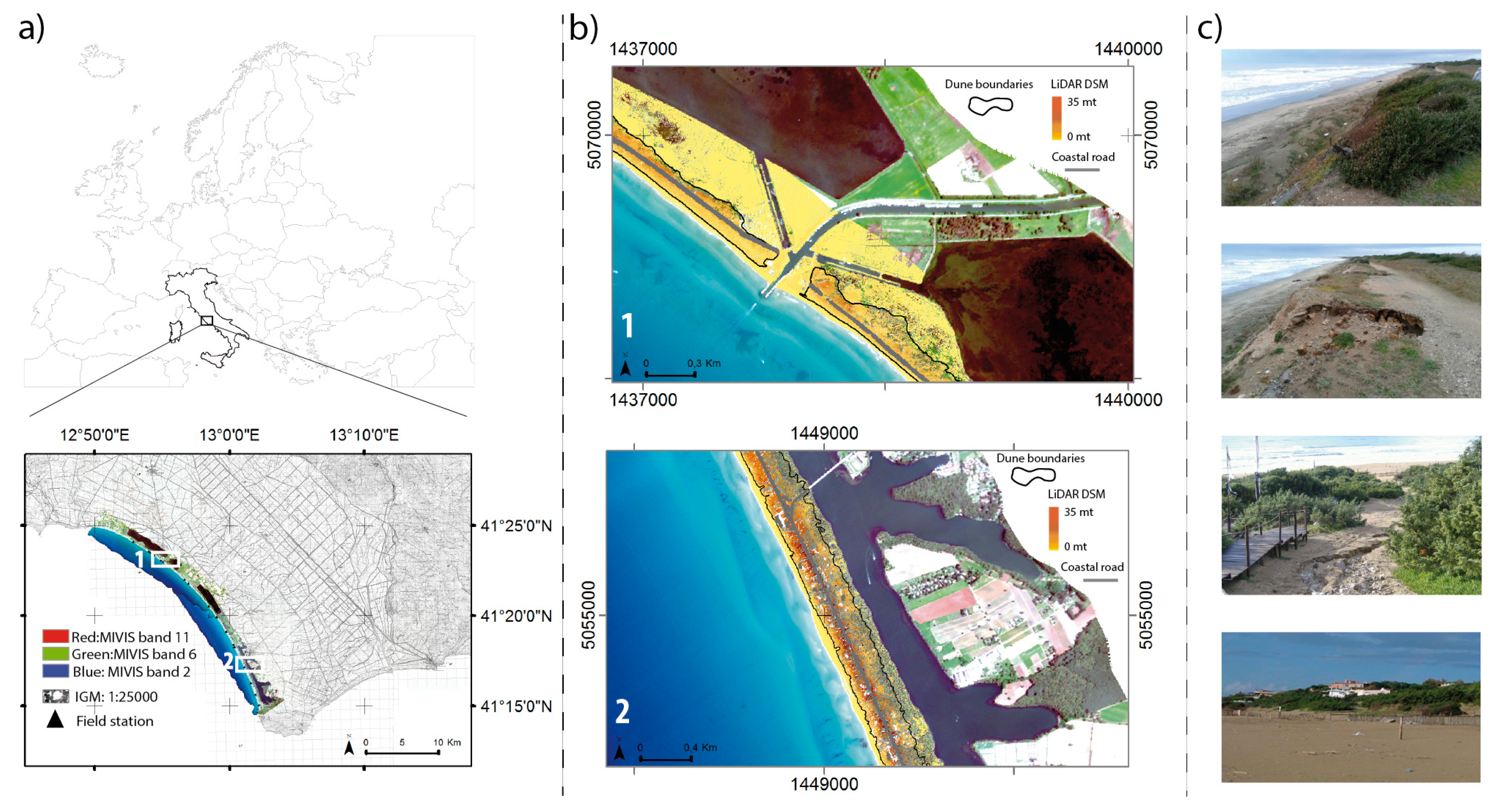
2. Study Area
3. Materials and Methods
3.1. Materials
3.1.1. Airborne LIDAR Altimeter
3.1.2. Hyperspectral Airborne Imagery
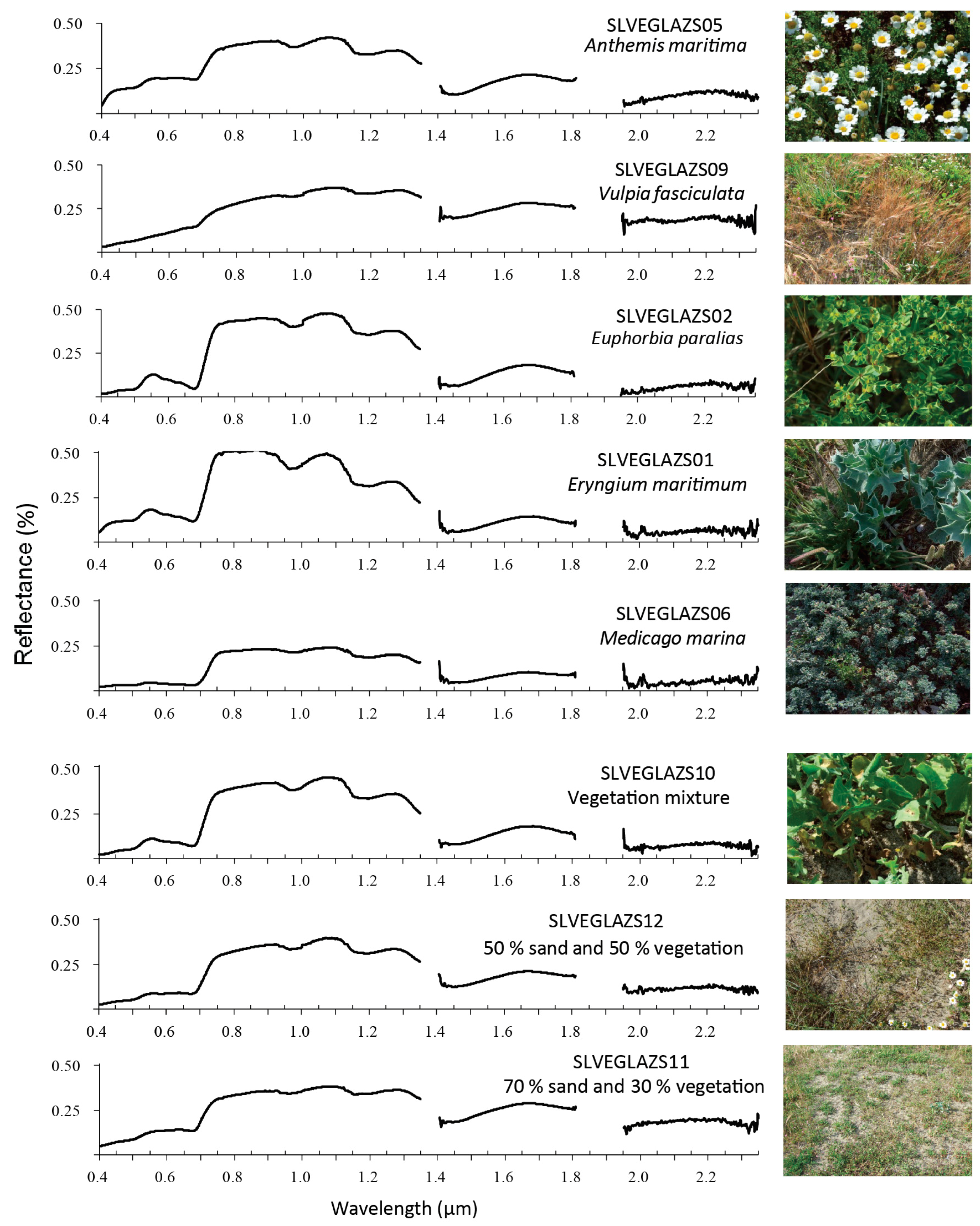
3.1.3. Field Measurements
3.2. Methodology
- -
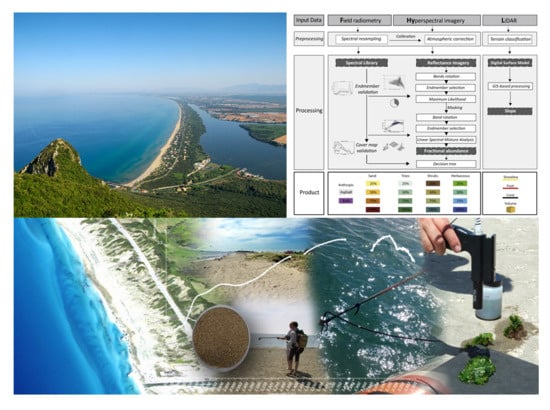
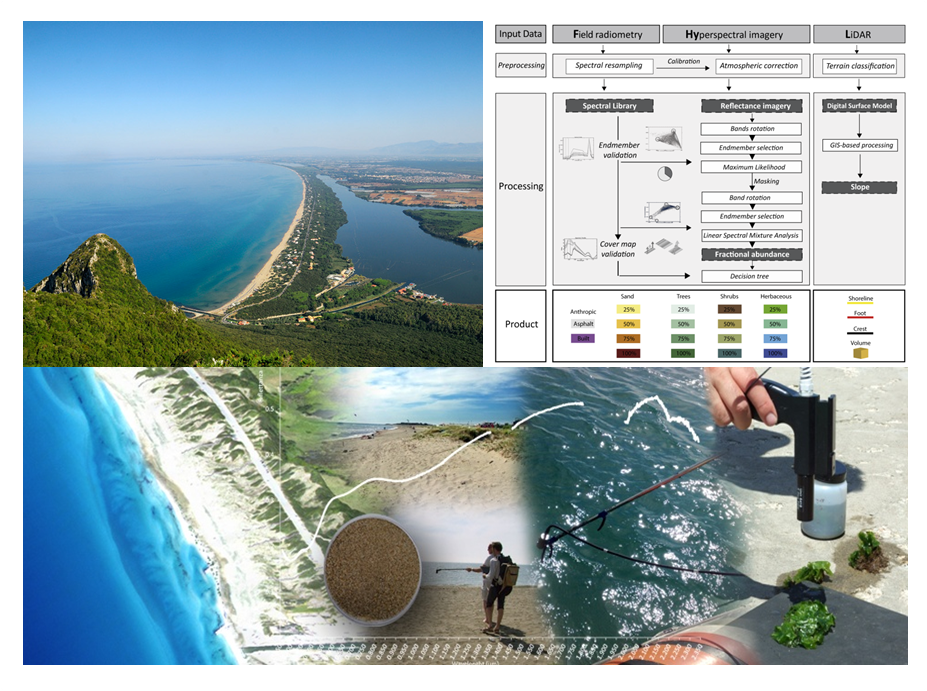
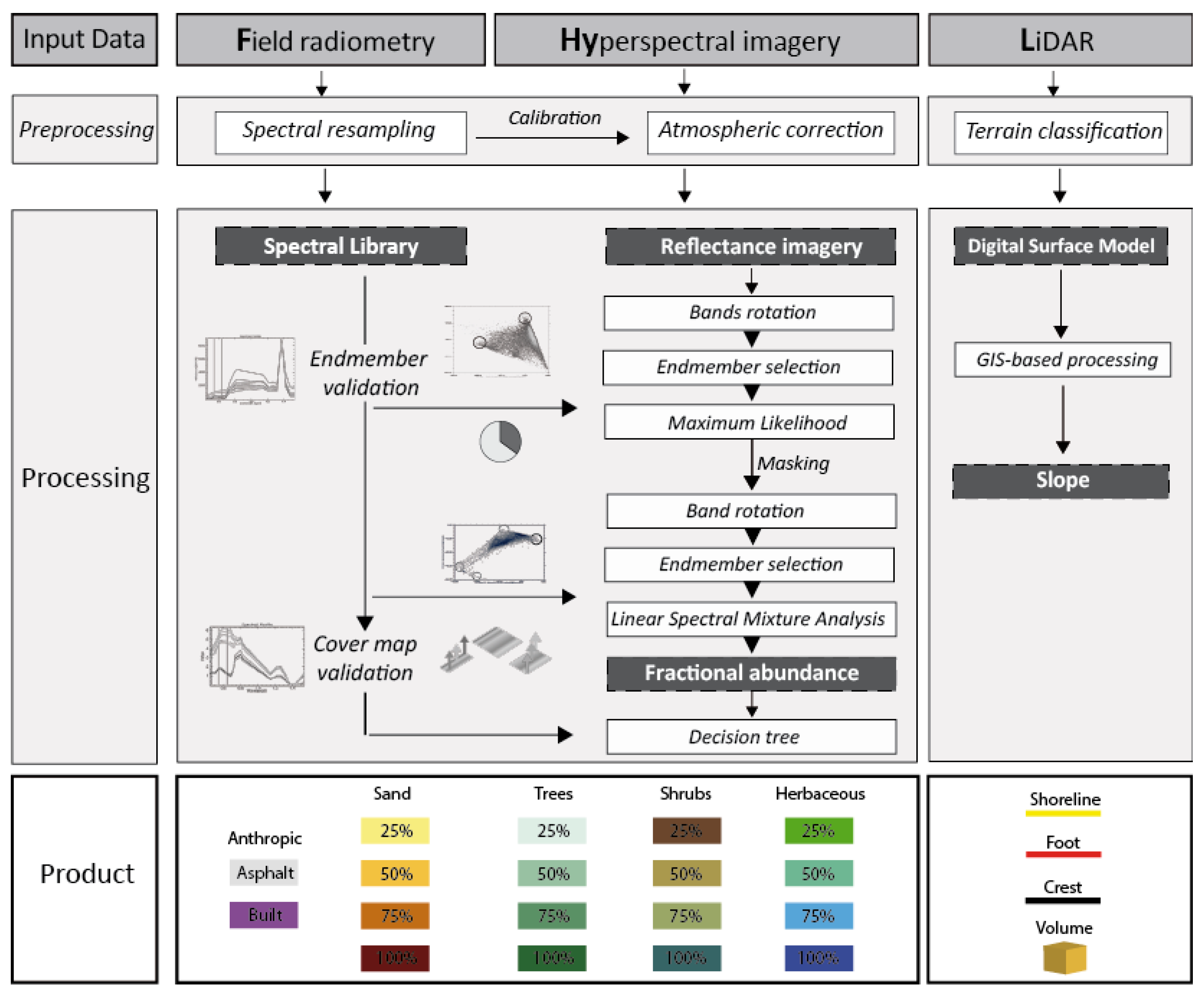
- step 1, a discrete pixel-based analysis to explore the whole system metrics and behavior. The processing is based on the algorithm named ‘FHyL (Field spectral libraries, airborne Hyperspectral images and LiDAR altimetry) module 3’, an algorithm comprising four main modules and two pre-processing steps: Each module differs according to the analyzed coastal sphere, i.e., the terrestrial or the aquatic, and according to the sensors’ data integration sequence [31,45];
- -
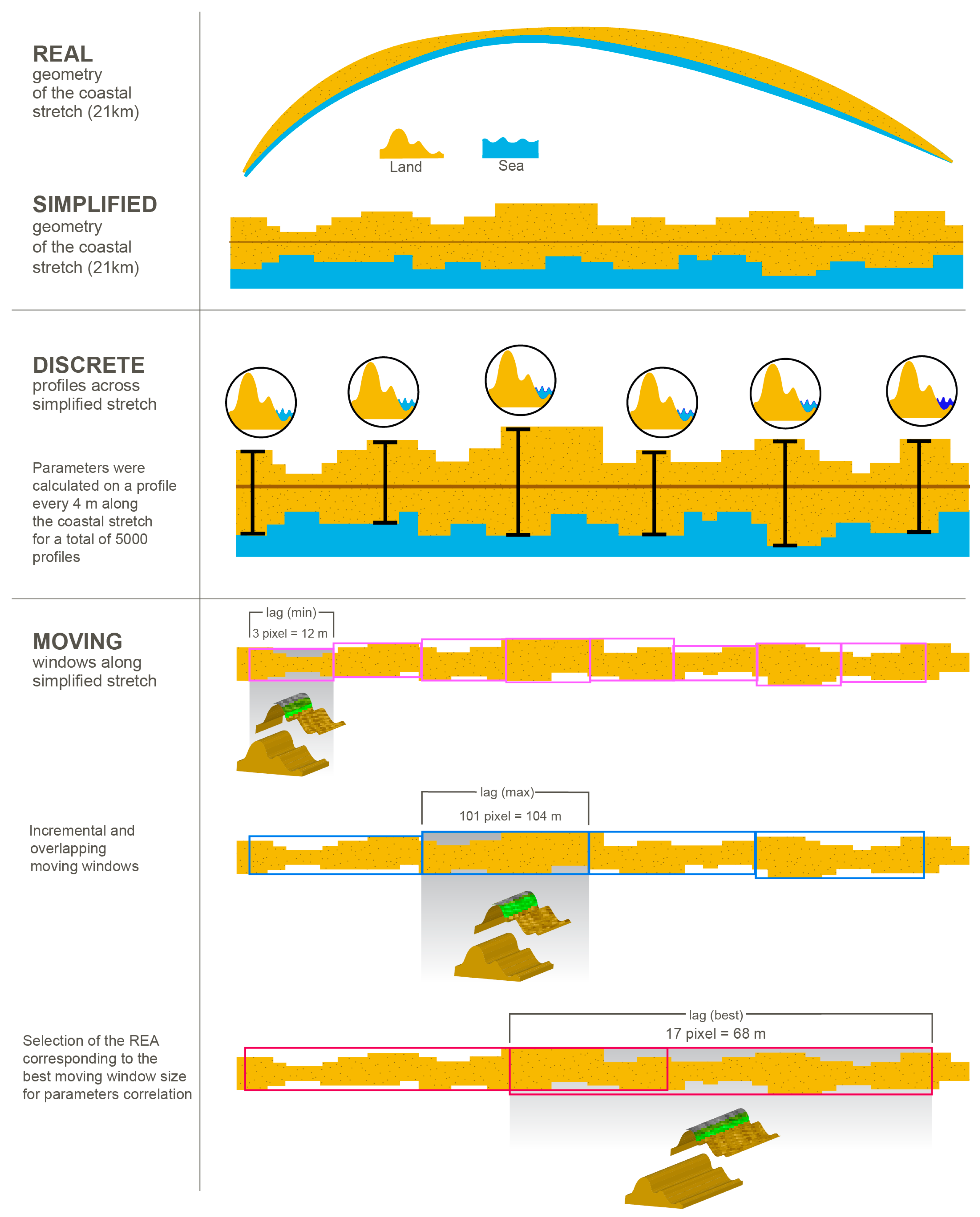
- step 2, a continuous lag-based analysis to explore the relationships between landscape cover and geomorphology;
- -
- step 3, a correlation analysis.
3.2.1. Step 1: Discrete Pixel-based Analysis
3.2.2. Step 2: Continuous Lag-Based Analysis
3.2.3. Step 3: Correlation Analysis between Landform and Landscape Metrics
4. Results
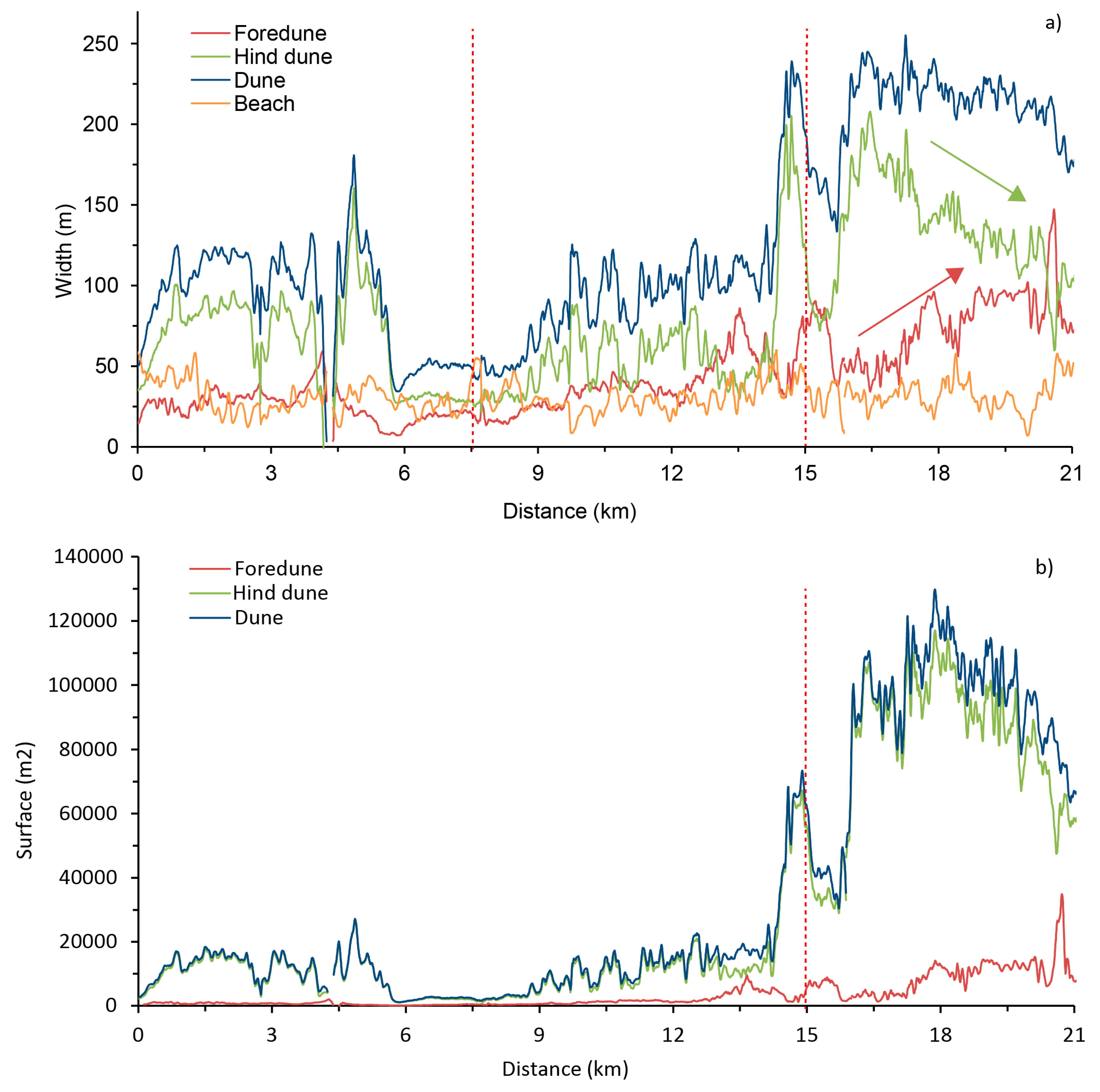
4.1. Step 1 and Step 2: Dune Morphology
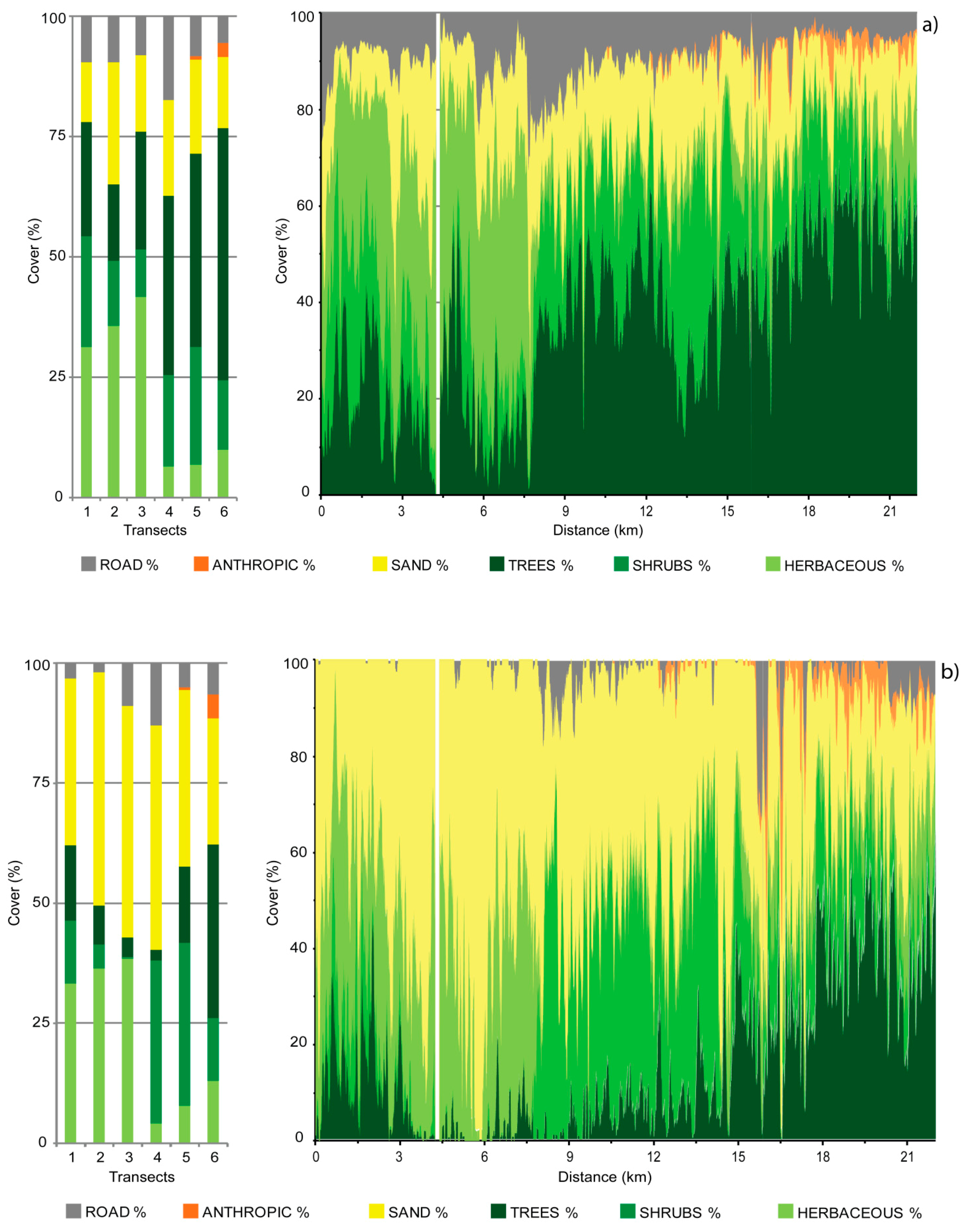
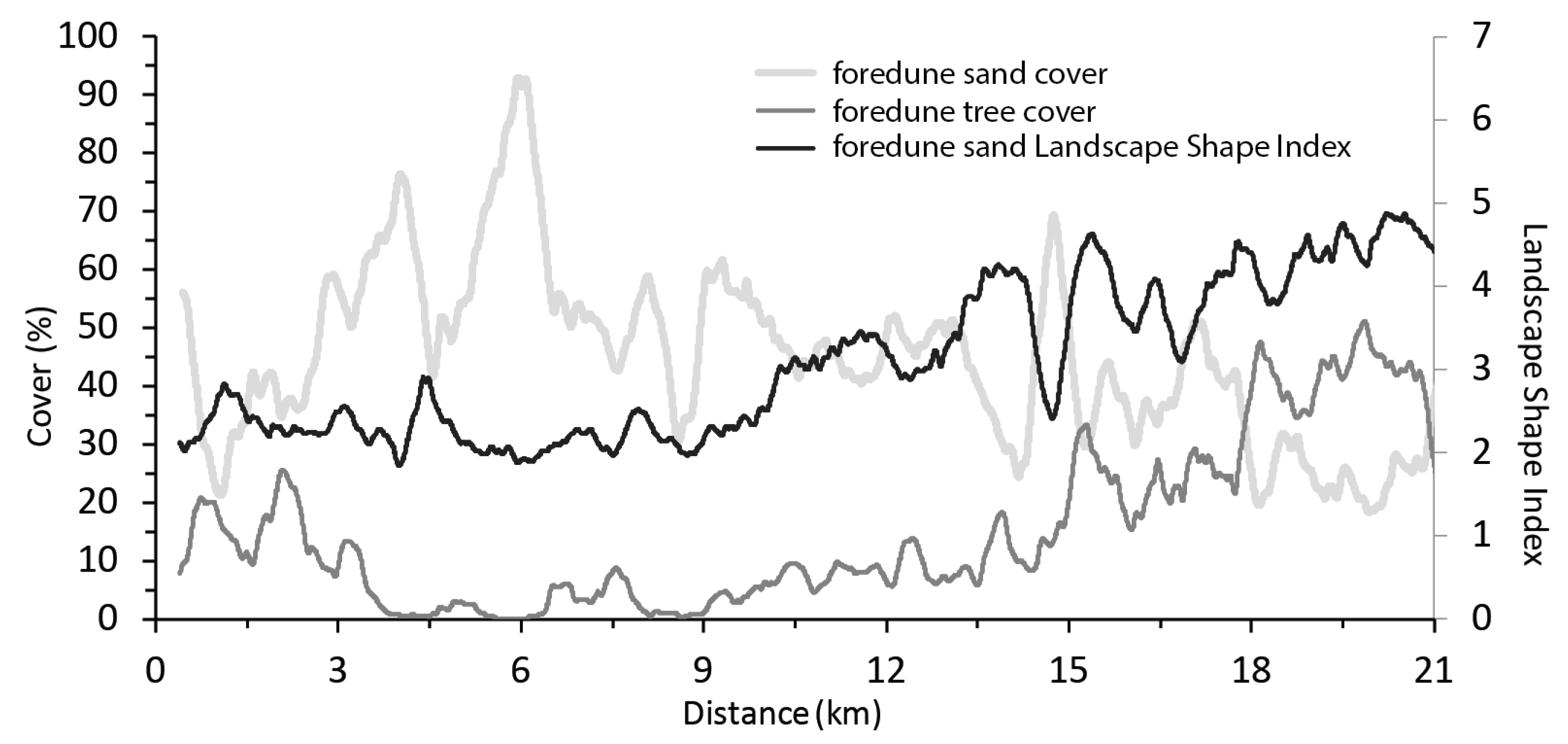
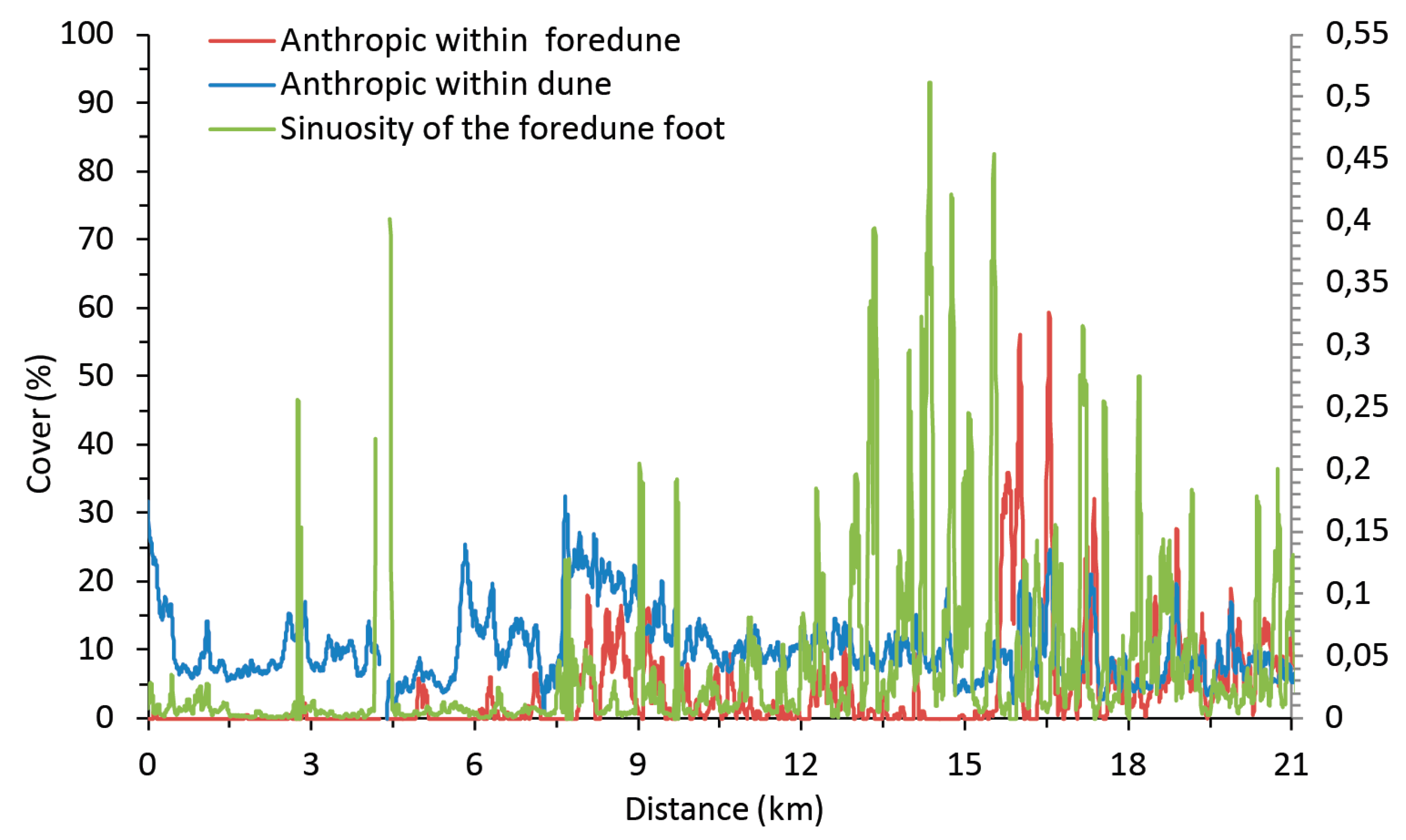
4.2. Step 1 and Step 2: Dune Cover Patterns
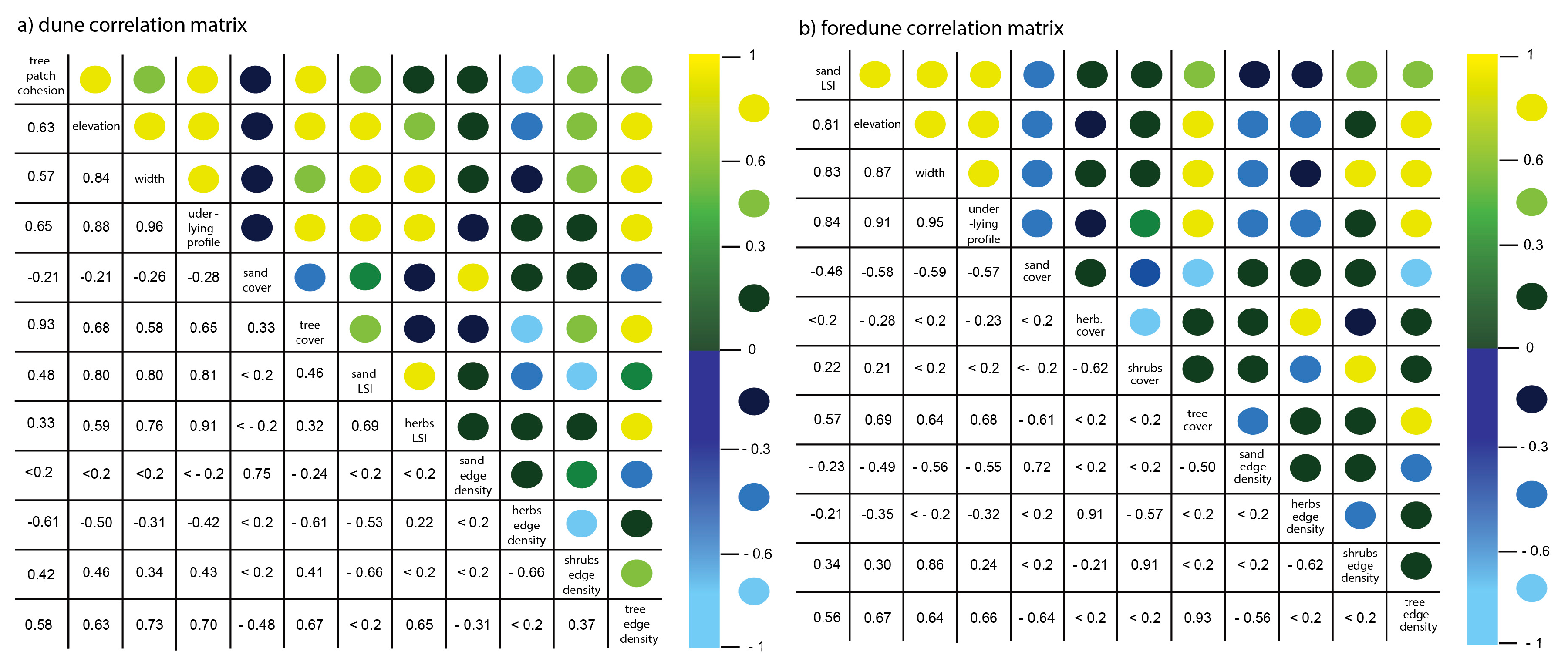
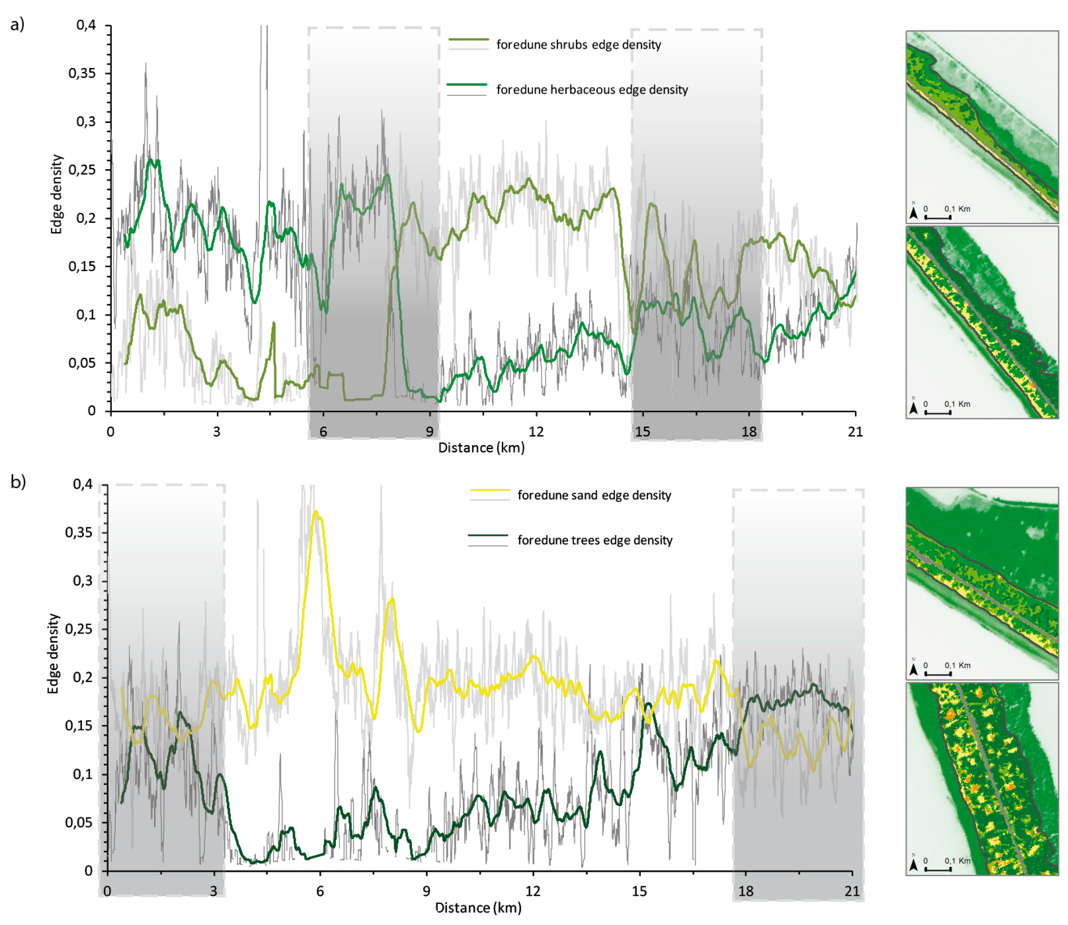
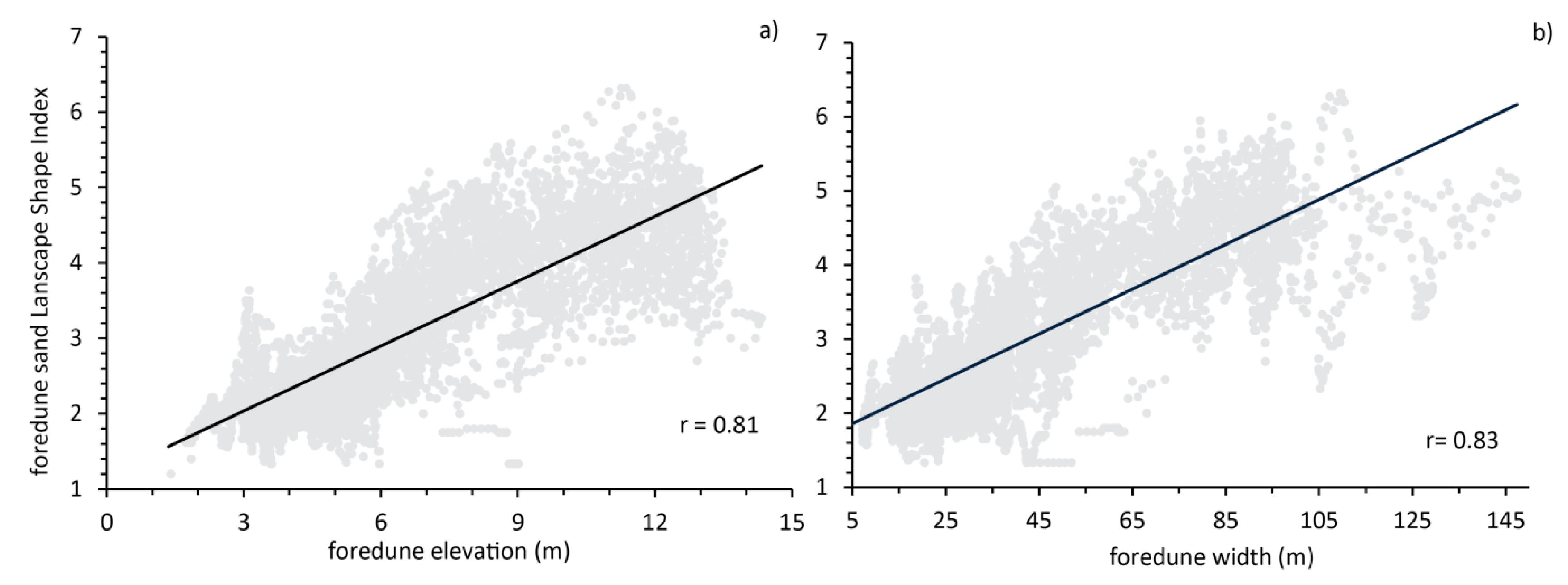
4.3. Step 3: Dune Landforms and Landscape Correlations
5. Discussion
6. Conclusions
Supplementary Materials
Author Contributions
Funding
Acknowledgments
Conflicts of Interest
References
- Baas, A.C.W.; Nield, J.M. Modelling vegetated dune landscapes. Geophys. Res. Lett. 2007, 34. [Google Scholar] [CrossRef]
- Barchyn, T.E.; Hugenholtz, C.H. Predicting vegetation-stabilized dune field morphology. Geophys. Res. Lett. 2013, 39. [Google Scholar] [CrossRef]
- Barchyn, T.E.; Hugenholtz, C.H. Reactivation of supply-limited dune fields from blowouts: A conceptual framework for state characterization. Geomorphology 2013, 201, 172–182. [Google Scholar] [CrossRef]
- Baas, A.C.W. Chaos, fractals and self-organization in coastal geomorphology: Simulating dune landscapes in vegetated environments. Geomorphology 2002, 48, 309–328. [Google Scholar] [CrossRef]
- Baas, A.C.W. Complex systems in aeolian geomorphology. Geomorphology 2007, 91, 311–331. [Google Scholar] [CrossRef]
- Kocurek, G.; Ewing, R.C. Aeolian dune field self-organization–implications for the formation of simple versus complex dune-field patterns. Geomorphology 2005, 72, 94–105. [Google Scholar] [CrossRef]
- Martínez, M.L.; Psuty, N.P.; Lubke, R.A. A Perspective on Coastal Dunes. In Coastal Dunes; Springer: Berlin/Heidelberg, Germany, 2008; pp. 3–10. [Google Scholar] [CrossRef]
- Ciccarelli, D.; Pinna, M.S.; Alquini, F.; Cogoni, D.; Ruocco, M.; Bacchetta, G.; Sarti, G.; Fenu, G. Development of a coastal dune vulnerability index for Mediterranean ecosystem: A useful tool for coastal managers? Estuar. Coast. Shelf Sci. 2017, 187, 84–95. [Google Scholar] [CrossRef]
- Corbau, C.; Simeoni, U.; Melchiorre, M.; Rodella, I.; Utizi, K. Regional variability of coastal dunes observed along the Emilia Romagna littoral Italy. Aeolian Res. 2015, 18, 169–183. [Google Scholar] [CrossRef]
- Hesp, P.A. A review of biological and geomorphological processes involved in the initiation and development of incipient foredunes. Proc. R. Soc. Edinb. 1989, 96, 181–201. [Google Scholar] [CrossRef]
- Hesp, P.A. Ecological processes and plant adaptations on coastal dunes. J. Arid Environ. 1991, 21, 165–191. [Google Scholar] [CrossRef]
- McAuliffe, J.R.; Hamerlynck, E.P.; Eppes, M.C. Landscape dynamics fostering the development and persistence of long-lived creosotebush (Larrea tridentata) clones in the Mojave desert. J. Arid Environ. 2007, 69, 96–126. [Google Scholar] [CrossRef]
- Keijsers, J.G.S.; De Groot, A.V.; Riksen, M.J.P.M. Vegetation and sedimentation on coastal foredunes. Geomorphology 2015, 228, 723–734. [Google Scholar] [CrossRef]
- Duran, O.; Moore, L.J. Vegetation controls on the maximum size of coastal dunes. Proc. Natl. Acad. Sci. USA 2013, 110, 17217–17222. [Google Scholar] [CrossRef] [PubMed]
- Zhang, L.; Baas, A.C. Mapping functional vegetation abundance in a coastal dune environment using a combination of LSMA and MLC: A case study at Kenfig NNR, Wales. Int. J. Remote Sens. 2012, 33, 5043–5071. [Google Scholar] [CrossRef]
- Lancaster, N.; Baas, A. Influence of vegetation cover on sand transport by wind: Field studies at Owens Lake, California. Earth Surf. Proc. Land. 1998, 23, 69–82. [Google Scholar] [CrossRef]
- Leenders, J.K.; Sterk, G.; Van Boxel, J.H. Modelling wind-blown sediment transport around single vegetation elements. Earth Surf. Proc. Land. 2011, 36, 1218–1229. [Google Scholar] [CrossRef]
- Pelletier, J.D.; Mitasova, H.; Harmon, R.S.; Overton, M. The effects of interdune vegetation changes on eolian dune field evolution: A numerical modeling case study at Jockey’s ridge, North Carolina, USA. Earth Surf. Proc. Land. 2009, 34, 1245–1254. [Google Scholar] [CrossRef]
- Nickling, W.G.; Neuman, C.M. Aeolian sediment transport. In Geomorphology of Desert Environments; Springer: Dordrecht, The Netherlands, 2009; pp. 517–555. [Google Scholar]
- Acosta, A.; Carranza, M.L.; Izzi, C.F. Combining land cover mapping of coastal dunes with vegetation analysis. Appl. Veg. Sci. 2005, 8, 133–138. [Google Scholar] [CrossRef]
- Acosta, A.; Ercole, S.; Stanisci, A.; Pillar, V.D.P.; Blasi, C. Coastal vegetation zonation and dune morphology in some Mediterranean ecosystems. J. Coast. Res. 2007, 1518–1524. [Google Scholar] [CrossRef]
- Mason, D.C.; Scott, T.R.; Dance, S.L. Remote sensing of intertidal morphological change in Morecambe Bay, U.K., between 1991 and 2007. Estuar. Coast. Shelf Sci. 2010, 87, 487–496. [Google Scholar] [CrossRef]
- Jones, T.G.; Coops, N.C.; Sharma, T. Assessing the utility of airborne hyperspectral and LiDAR data for species distribution mapping in the coastal Pacific Northwest, Canada. Remote Sens. Environ. 2010, 114, 2841–2852. [Google Scholar] [CrossRef]
- Zalasiewicz, J.; Waters, C.N.; Head, M.J.; Poirier, C.; Summerhayes, C.P.; Leinfelder, R.; Grinevald, J.; Steffen, W.; Syvitski, J.P.M.; Haff, P.; et al. A formal Anthropocene is compatible with but distinct from its diachronous anthropogenic counterparts: A response to W.F. Ruddiman’s ‘three-flaws in defining a formal Anthropocene’. Prog. Phys. Geog. 2019, 43, 319–333. [Google Scholar] [CrossRef]
- Cappucci, S.; Scarcella, D.; Rossi, L.; Taramelli, A. Integrated Coastal Zone Management at Marina di Carrara Harbor: Sediment management and policymaking. Ocean Coast. Manag. 2011, 54, 277–289. [Google Scholar] [CrossRef]
- Pelletier, J.D.; Brad Murray, A.; Pierce, J.L.; Bierman, P.R.; Breshears, D.D.; Crosby, B.T.; Ellis, M.; Foufoula-Georgiou, E.; Heimsath, A.M.; Houser, C.; et al. Forecasting the response of Earth’s surface to future climatic and land use changes: A review of methods and research needs. Earth’s Future 2015, 3, 220–251. [Google Scholar] [CrossRef]
- Yousefi Lalimi, F.; Silvestri, S.; Moore, L.J.; Marani, M. Coupled topographic and vegetation patterns in coastal dunes: Remote sensing observations and ecomorphodynamic implications. J. Geophys. Res. Biogeosci. 2017, 122, 119–130. [Google Scholar] [CrossRef]
- Ibrahim, E.; Monbaliu, J. Suitability of spaceborne multispectral data for inter-tidal sediment characterization: A case study. Estuar. Coast. Shelf Sci. 2011, 92, 437–445. [Google Scholar] [CrossRef]
- Jin, H.X.; Eklundh, L. A physically based vegetation index for improved monitoring of plant phenology. Remote Sens. Environ. 2014, 152, 512–525. [Google Scholar] [CrossRef]
- Mancini, F.; Dubbini, M.; Gattelli, M.; Stecchi, F.; Fabbri, S.; Gabbianelli, G. Using un- manned aerial vehicles (UAV) for high-resolution reconstruction of topography: The structure from motion approach on coastal environments. Remote Sens. 2013, 5, 6880–6898. [Google Scholar] [CrossRef]
- Valentini, E.; Taramelli, A.; Filipponi, F.; Giulio, S. An effective procedure for EUNIS and Natura 2000 habitat type mapping in estuarine ecosystems integrating ecological knowledge and remote sensing analysis. Ocean Coast. Manag. 2015, 108, 52–64. [Google Scholar] [CrossRef]
- Taramelli, A.; Valentini, E.; Cornacchia, L.; Bozzeda, F. A hybrid power law approach for spatial and temporal pattern analysis of salt marsh evolution. J. Coast. Res. 2017, 77, 62–72. [Google Scholar] [CrossRef]
- Cracknell, A. Remote sensing techniques in estuaries and coastal zones an update. Int. J. Remote Sens. 1999, 20, 485–496. [Google Scholar] [CrossRef]
- Mumby, P.J.; Edwards, A.J. Mapping marine environments with IKONOS imagery-Enhanced spatial resolution can deliver greater thematic accuracy. Remote Sens. Environ. 2002, 82, 248–257. [Google Scholar] [CrossRef]
- Taramelli, A.; Valentini, E.; Cornacchia, L.; Monbaliu, J.; Sabbe, K. Self-organized processes between salt marsh vegetation patterns and channel network in a tidal landscape. J. Geophys. Res.-Earth 2018, 123, 2714–2731. [Google Scholar] [CrossRef]
- Manzo, C.; Valentini, E.; Taramelli, A.; Filipponi, F.; Disperati, L. Spectral characterization of coastal sediments using Field Spectral Libraries, Airborne Hyperspectral Images and Topographic LiDAR Data (FHyL). Int. J. Appl. Earth Obs. 2015, 36, 54–68. [Google Scholar] [CrossRef]
- Cappucci, S.; Valentini, E.; Del Monte, M.; Paci, M.; Filipponi, F.; Taramelli, A. Detection of natural and anthropic features on small islands. J. Coast. Res. 2017, 77, 74–88. [Google Scholar] [CrossRef]
- Zhang, X.; Liao, C.; Li, J.; Sun, Q. Fractional vegetation cover estimation in arid and semi-arid environments using HJ-1 satellite hyperspectral data. Int. J. Appl. Earth Obs. 2013, 21, 506–512. [Google Scholar] [CrossRef]
- Rainey, M.P.; Tyler, A.N.; Gilvear, D.J.; Bryant, R.G.; McDonald, P. Mapping intertidal estuarine sediment grain size distributions through airborne remote sensing. Remote Sens. Environ. 2003, 86, 480–490. [Google Scholar] [CrossRef]
- Small, C.; Steckler, M.; Seeber, L.; Akhter, S.H.; Goodbred, S., Jr.; Mia, B.; Imam, B. Spectroscopy of sediments in the Ganges-Brahmaputra delta: Spectral effects of moisture, grain size and lithology. Remote Sens. Environ. 2009, 113, 342–361. [Google Scholar] [CrossRef]
- Bazzichetto, M.; Malavasi, M.; Acosta, A.T.R.; Carranza, M.L. How does dune morphology shape coastal EC habitats occurrence? A remote sensing approach using airborne LiDAR on the Mediterranean coast. Ecol. Indic. 2016, 71, 618–626. [Google Scholar] [CrossRef]
- Brock, J.C.; Purkis, S.J. The emerging role of lidar remote sensing in coastal research and resource management. J. Coast. Res. 2009, 1–5. [Google Scholar] [CrossRef]
- Sallenger, A.H., Jr.; Krabill, W.B.; Swift, R.N.; Brock, J.; List Mark Hansen, J.; Holman, R.A.; Manizade, S.; Sontag, J.; Meredith, A.; Morgan, K.; et al. Evaluation of airborne topographic Lidar for quantifying beach changes. J. Coast. Res. 2003, 19, 125–133. [Google Scholar]
- Chust, G.; Galparsoro, I.; Borja, A.; Franco, J.; Uriarte, A. Coastal and estuarine habitat mapping, using LIDAR height and intensity and multi-spectral imagery. Estuar. Coast. Shelf Sci. 2008, 78, 633–643. [Google Scholar] [CrossRef]
- Taramelli, A.; Valentini, E.; Innocenti, C.; Cappucci, S. FHyL: Field spectral libraries, airborne hyperspectral images and topographic and bathymetric LiDAR data for complex coastal mapping. Geoscience and Remote Sensing Symposium (IGARSS). In Proceedings of the 2013 IEEE International Geoscience and Remote Sensing Symposium-IGARSS, Melbourne, Australia, 21–26 July 2013; pp. 2270–2273. [Google Scholar] [CrossRef]
- Pascucci, V.; De Falco, G.; Del Vais, C.; Melis, R.; Sanna, I.; Andreucci, S. Climate Changes And Human Impact on The Mistras Coastal Barrier System (W Sardinia, Italy). Mar. Geol. 2018, 395, 271–284. [Google Scholar] [CrossRef]
- Pascucci, V.; Frulio, G.; Andreucci, S. New estimation of the post Little Ice Age Relative Sea Level Rise. Geosciences 2019, 9, 348. [Google Scholar] [CrossRef]
- Campo, V.; La Monica, G.B. Le dune costiere oloceniche prossimali lungo il litorale del Lazio. Studi Costieri 2006, 11, 31–42. [Google Scholar]
- Carboni, M.; Santoro, R.; Acosta, A.T.R. Are some communities of the coastal dune zonation more susceptible to alien plant invasion? J. Plant. Ecol. 2010, 3, 139–147. [Google Scholar] [CrossRef]
- Pascucci, V.; Cappucci, S.; Andreucci, S.; Donda, F. Sedimentary features of the offshore part of the la Pelosa Beach (Sardinia, Italy). Rend. Line Soc. Geol. Ital. 2008, 2, 1–3. [Google Scholar]
- Pallottini, E.; Cappucci, S. Beach—Dune system interaction and evolution. Rend. Soc. Geo. Ital. 2009, 8, 87–97. [Google Scholar]
- Conti, M.; Cappucci, S.; La Monica, G.B. Sediment dynamic of nourished sandy beaches. Rend. Line Soc. Geol. Ital. 2009, 8, 31–38. [Google Scholar]
- Quadros, N.D.; Collier, P.A.; Fraser, C.S. Integration of bathymetric and topographic LiDAR: A preliminary investigation. ISPRS J. Photogramm. Remote Sens. 2008, 37, 1299–1304. [Google Scholar]
- Allegrini, A.; Anselmi, S.; Cavalli, R.M.; Manes, F.; Pignatti, S. Multiscale integration of satellite, airborne and field data for Mediterranean vegetation studies in the natural area of the Castelporziano Estate (Rome). Ann. Geophys. 2005, 49, 167–175. [Google Scholar]
- Innocenti, C.; Filipponi, F.; Valentini, E.; Taramelli, A. Multisensory data fusion methods for the estimation of beach sediment features: Mineralogical, grain size and moisture, Geoscience and Remote Sensing Symposium (IGARSS). In Proceedings of the 2013 IEEE International Geoscience and Remote Sensing Symposium-IGARSS, Melbourne, Australia, 21–26 July 2013; pp. 3064–3067. [Google Scholar] [CrossRef]
- Sorichetta, A.; Seeber, L.; Taramelli, A.; McHugh, C.M.G.; Cormier, M.H. Geomorphic evidence for tilting at a continental transform: The Karamusel basin along the North Anatolian Fault, Turkey. Geomorphology 2010, 119, 221–231. [Google Scholar] [CrossRef]
- Sousa, D.; Small, C. Global cross-calibration of Landsat spectral mixture models. Remote Sens. Environ. 2017, 192, 139–149. [Google Scholar] [CrossRef]
- Small, C. The Landsat ETM+ spectral mixing space. Remote Sens. Environ. 2004, 93, 1–17. [Google Scholar] [CrossRef]
- Combe, J.P.; Launeau, P.; Carrère, V.; Despan, D.; Méléder, V.; Barillé, L.; Sotin, C. Mapping microphytobenthos biomass by non-linear inversion of visible-infrared hyperspectral images. Remote Sens. Environ. 2005, 98, 371–387. [Google Scholar] [CrossRef]
- Roberts, D.; Green, R.; Adams, J. Temporal and spatial patterns in vegetation and atmospheric properties from AVIRIS. Remote Sens. Environ. 1997, 62, 223–240. [Google Scholar] [CrossRef]
- Metternicht, G.; Fermont, A. Estimating erosion surface features by linear mixture modeling. Remote Sens. Environ. 1998, 64, 254–265. [Google Scholar] [CrossRef]
- McGarigal, K.; Cushman, S.A.; Ene, E. FRAGSTATS v4: Spatial Pattern Analysis Program for Categorical and Continuous Maps. University of Massachusetts, Amherst. Computer Software Program Produced by the Authors at the Uni-versity of Massachusetts. 2012. Available online: https://www.umass.edu/landeco/research/fragstats/fragstats.html (accessed on 8 April 2020).
- Pallottini, E.; Cappucci, S.; Taramelli, A.; Innocenti, C.; Screpanti, A. Variazioni morfologiche stagionali del sistema spiaggia-duna del Parco Nazionale del Circeo. Studi Costieri 2010, 17, 105–124. [Google Scholar]
- Baas, A.C.; Nield, J.M. Ecogeomorphic state variables and phase-space construction for quantifying the evolution of vegetated aeolian landscapes. Earth Surf. Proc. Land. 2010, 35, 717–773. [Google Scholar] [CrossRef]
- Finkl, C.W. Coastal classification: Systematic approaches to consider in the development of a comprehensive scheme. J. Coast. Res. 2003, 20, 166–213. [Google Scholar] [CrossRef]
- Taramelli, A.; Cappucci, S.; Valentini, E.; Rossi, L.; Lisi, I. Nearshore Sandbar Classification of Sabaudia (Italy) with LiDAR Data: The FHyL Approach. Remote Sens. 2020, 12, 1053. [Google Scholar] [CrossRef]
- Nield, J.M.; Baas, A.C.W. The influence of different environmental and climatic conditions on vegetated aeolian dune landscape development and response. Glob. Planet. Change 2008, 64, 76–92. [Google Scholar] [CrossRef]
- Williams, M.; Zalasiewicz, J.; Waters, N.C.; Leinfelder, R. The palaeontological record of the Anthropocene. Geol. Today 2018, 34, 188–193. [Google Scholar] [CrossRef]
- Lewis, S.L.; Maslin, M.A. Defining the Anthropocene. Nature 2015, 519, 171–180. [Google Scholar] [CrossRef] [PubMed]


| LiDAR HawkEye II | |
|---|---|
| Topographic Frequency | 64,000 Hz |
| Altitude | From 250 to 500 m |
| Swath | From 100 to 330 m |
| Topographic point density | From 1 to 4 points for m2 |
| Accuracy of Topographic survey | Horizontal: ±0.5 m (Vertical: ±0.15 m |
| MIVIS – Multispectral Infrared Visible Imaging Spectrometer | ||
|---|---|---|
| Wavelength (μm) | Spectral resolution (μm) | |
| Spectrometer I, VIS | 0.4–0.8 | 0.2 in 20 bands |
| Spectrometer II, NIR | 1.2–1.5 | 0.5 in 8 bands |
| Spectrometer III, MIR | 2.0–2.5 | 0.09 in 64 bands |
| Spectrometer IV, TIR | 8.2–12.7 | 3.4–5.4 in 10 bands |
| scan/s 25 (1500 m flight altitude) | 3 × 3 m spatial resolution | |
| Digital accuracy | 12 bit × pixel, ±1 bit | |
| Primary Parameter (units) | How to Calculate |
|---|---|
| Slope (deg) | Maximum change in elevation over the distance between the cell and its eight neighbors |
| Crest (m) | Maximum of dune ridge elevation |
| Foot (m) | Foot results from defining a threshold on the slope |
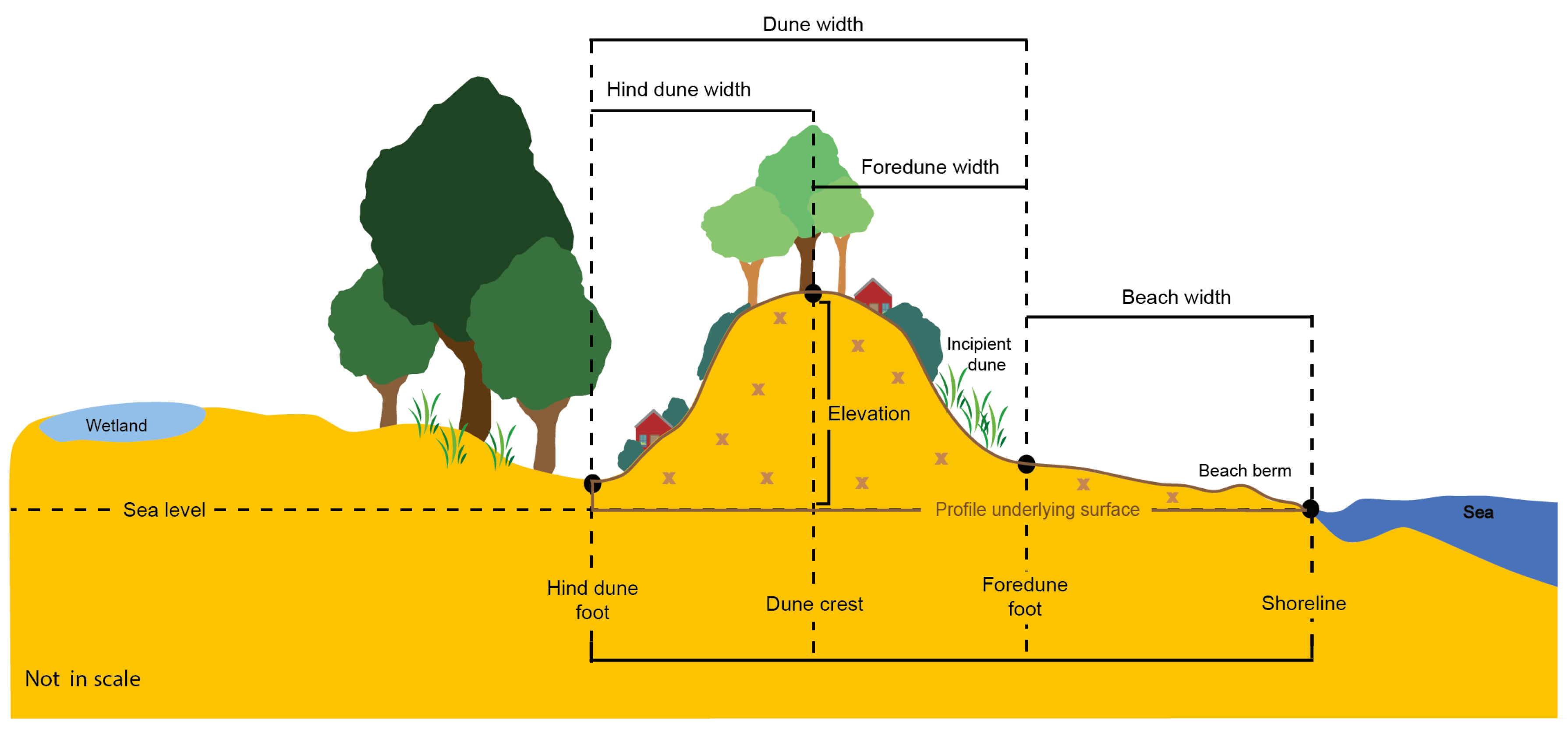
| Width (m) | By using the horizontal plane referred to mean sea level for the following distances: from the shoreline to the foredune foot (beach) from the foredune foot to the crest (foredune) from the crest to the hind dune foot (hind dune) from the foredune foot to the hind dune foot (dune) |
| Profile underlying the surface (m2) | The signed area, bounded by the elevation profile of each transect, corresponds to the integral of the elevation profile. Each profile has been separately calculated along the transect for the beach, foredune, and hind dune |
| Fractional Abundances (%) | Combining a maximum likelihood classification (MLL) and a linear spectral mixing analysis (LSMA) |
| Detailed cover map (classified map) | Using a decision tree to apply a threshold on fractional abundances (fraction > 60%) |
| Primary Parameter (unit) | How to Calculate (in the Moving Window) |
|---|---|
| Elevation (m) | As average value |
| Sinuosity | As average value of the crest and foot lines |
| Width (m2) | As average value |
| Profile underlying surface | As average value of the elevation profiles’ integrals |
| Cover percentage (%) | Cover percentage referred to the window extent |
| Edge Density (ED) | Edge density of the cover patches. It standardizes the edge to a per-unit-area basis that facilitates comparisons among landscapes of varying size. |
| Landscape Shape Index (LSI) | Measure of the perimeter-to-area ratio for the whole landscape. The minimum value of LSI is always equal to 1 when the landscape consists of a single patch. |
| Mean fractal dimension | Fractal dimension of each patch |
| Aggregation index | The ratio of the observed number of like adjacencies to the maximum possible number of like adjacencies given the proportion of the landscape comprising each patch type, given as a percentage. |
| Effective mesh size | Mesh size refers to the cumulative patch area distribution and is the size of the patches when the corresponding patch type is subdivided into S patches, where S is the value of the splitting index. |
| Patch Cohesion Index (PCI) | Measures of the connectivity of patch typologies. It takes into account the number of patches, the surface, and its perimeter |
| Distance along Stretch (km) | Foredune Width (m) | Hind dune Width (m) | Beach Width (m) | Profile Underlying the Surface (m2) | Elevation (m) |
|---|---|---|---|---|---|
| 1.5 | 25.4 | 100 | 29.7 | 581.6 | 4.1 |
| 4.5 | 36.0 | 89.5 | 12.7 | 868.0 | 4.2 |
| 7.5 | 21.2 | 28 | 42.4 | 410.5 | 5.0 |
| 10.5 | 41.5 | 70.6 | 23.1 | 1313.1 | 4.9 |
| 13.5 | 86.7 | 27.5 | 26.8 | 9143.5 | 7.7 |
| 16.5 | 36.0 | 203.7 | 26.1 | 1111.5 | 5.3 |
| 19.5 | 98.5 | 124.6 | 30.7 | 12,492.4 | 11.4 |
© 2020 by the authors. Licensee MDPI, Basel, Switzerland. This article is an open access article distributed under the terms and conditions of the Creative Commons Attribution (CC BY) license (http://creativecommons.org/licenses/by/4.0/).
Share and Cite
Valentini, E.; Taramelli, A.; Cappucci, S.; Filipponi, F.; Nguyen Xuan, A. Exploring the Dunes: The Correlations between Vegetation Cover Pattern and Morphology for Sediment Retention Assessment Using Airborne Multisensor Acquisition. Remote Sens. 2020, 12, 1229. https://doi.org/10.3390/rs12081229
Valentini E, Taramelli A, Cappucci S, Filipponi F, Nguyen Xuan A. Exploring the Dunes: The Correlations between Vegetation Cover Pattern and Morphology for Sediment Retention Assessment Using Airborne Multisensor Acquisition. Remote Sensing. 2020; 12(8):1229. https://doi.org/10.3390/rs12081229
Chicago/Turabian StyleValentini, Emiliana, Andrea Taramelli, Sergio Cappucci, Federico Filipponi, and Alessandra Nguyen Xuan. 2020. "Exploring the Dunes: The Correlations between Vegetation Cover Pattern and Morphology for Sediment Retention Assessment Using Airborne Multisensor Acquisition" Remote Sensing 12, no. 8: 1229. https://doi.org/10.3390/rs12081229
APA StyleValentini, E., Taramelli, A., Cappucci, S., Filipponi, F., & Nguyen Xuan, A. (2020). Exploring the Dunes: The Correlations between Vegetation Cover Pattern and Morphology for Sediment Retention Assessment Using Airborne Multisensor Acquisition. Remote Sensing, 12(8), 1229. https://doi.org/10.3390/rs12081229