Flexible Hierarchical Gaussian Mixture Model for High-Resolution Remote Sensing Image Segmentation

Abstract
1. Introduction
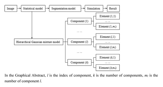
2. The Proposed Algorithm
2.1. Image Model
2.2. Segmentation Model
2.3. Optimal Segmentation
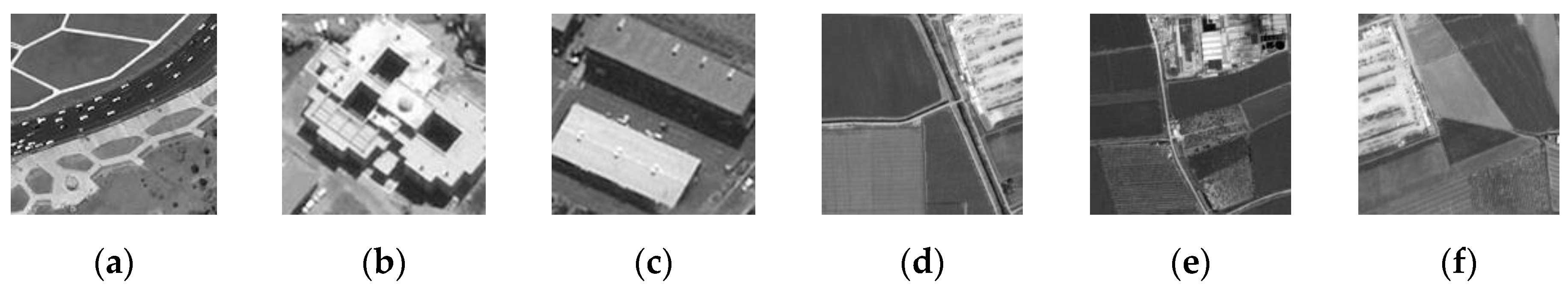
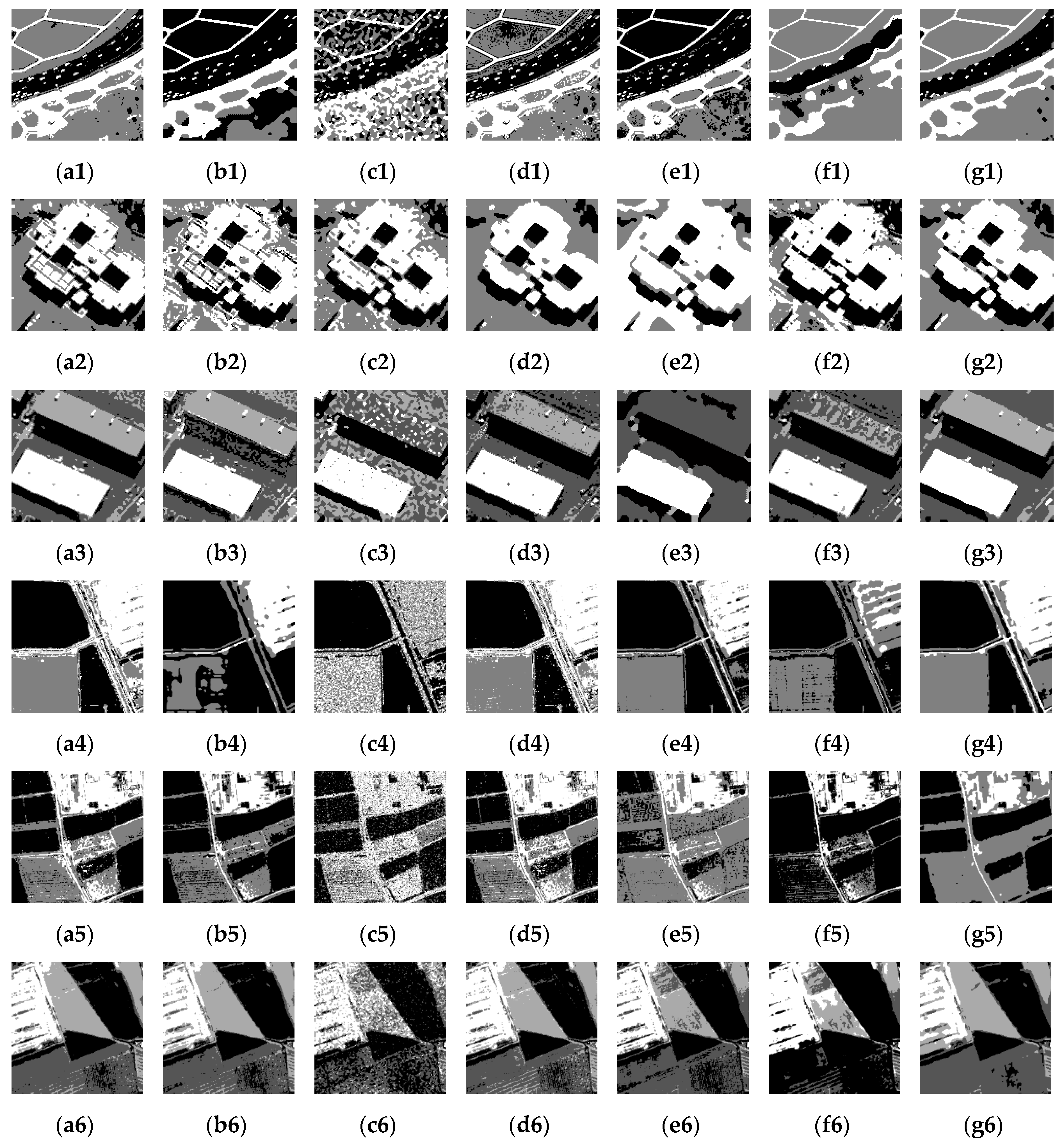
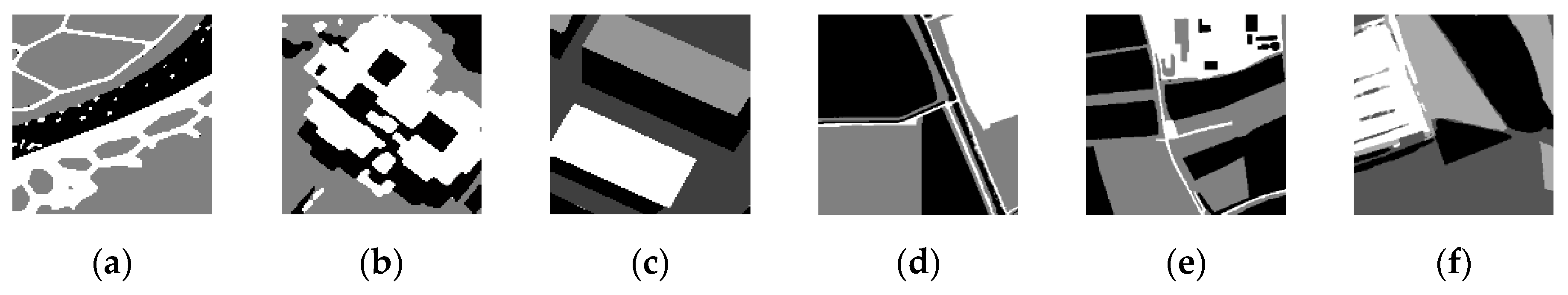
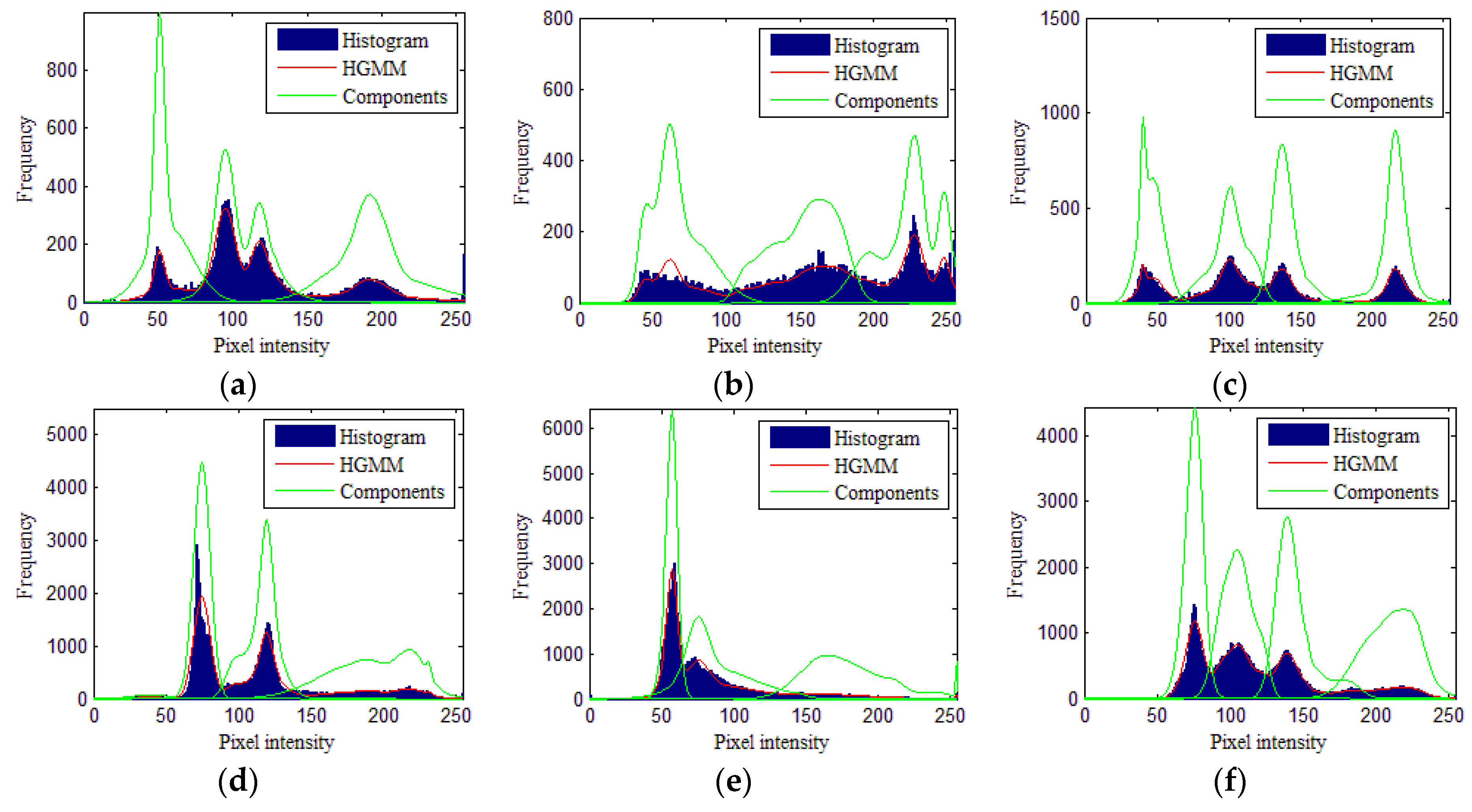
3. Results
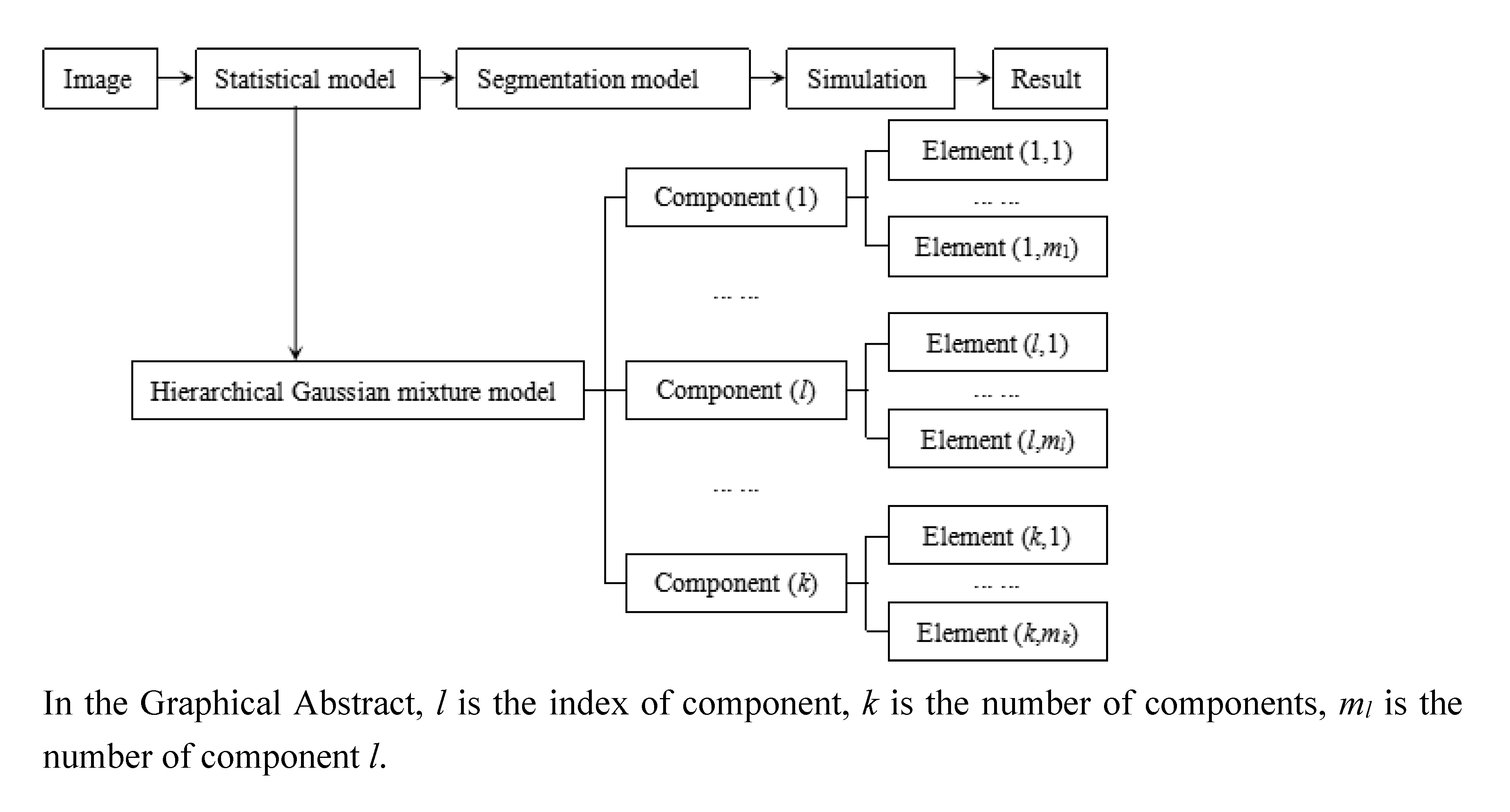
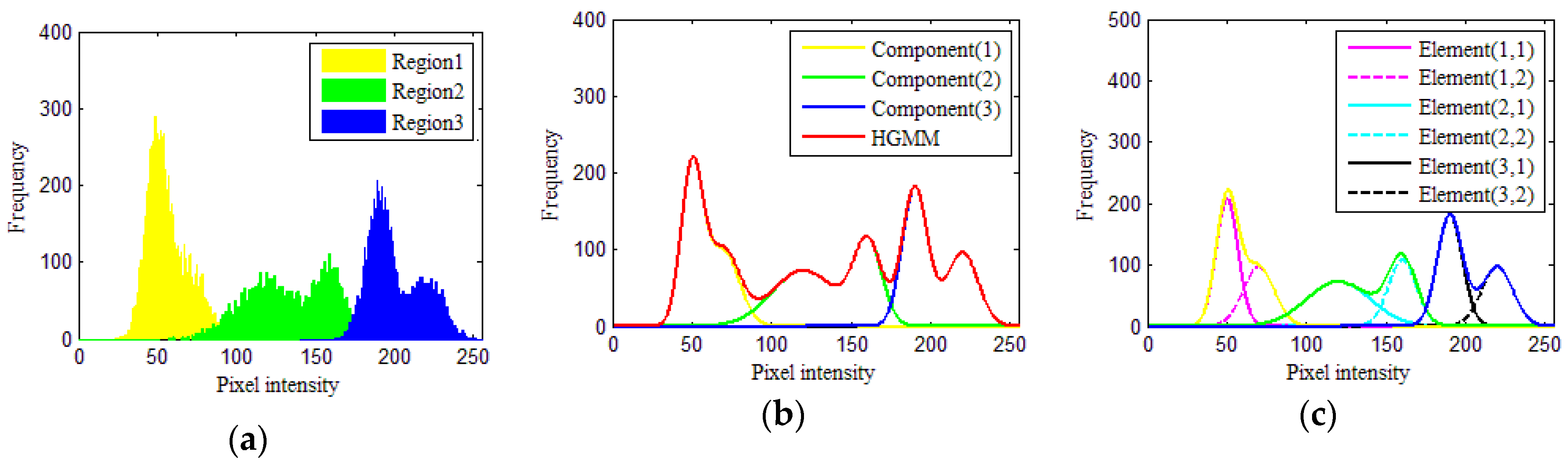
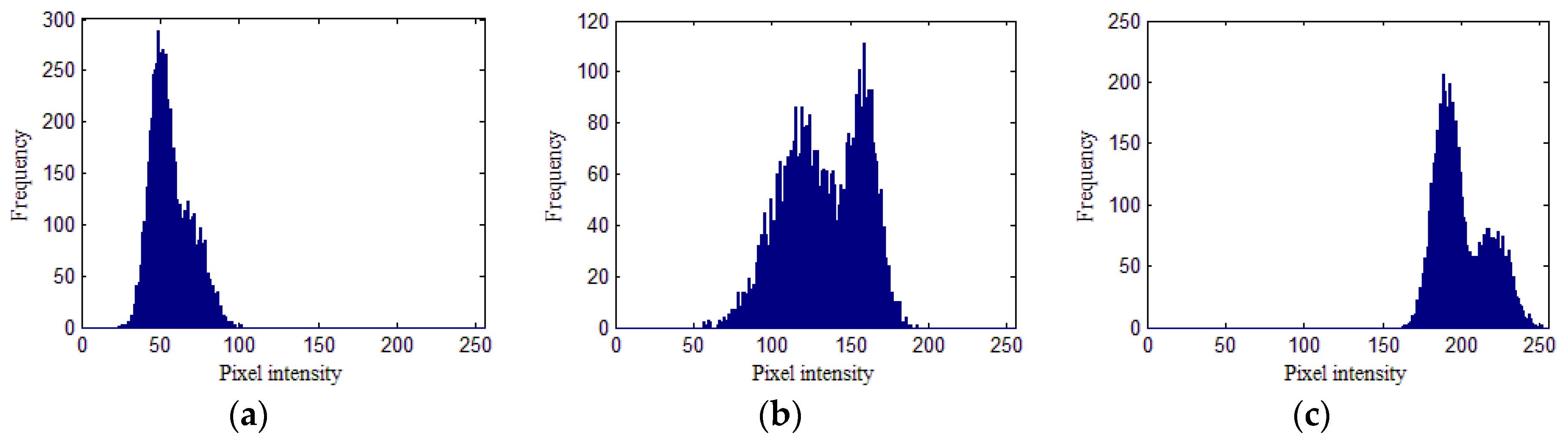
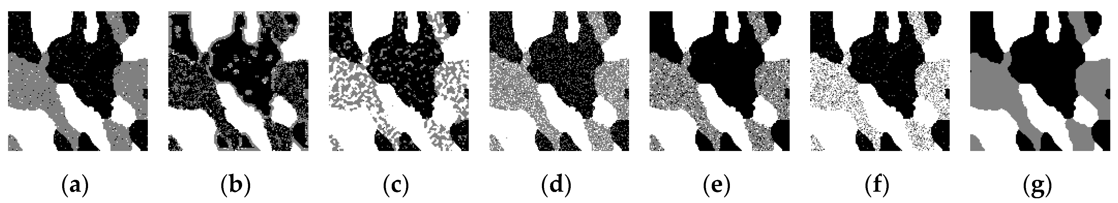
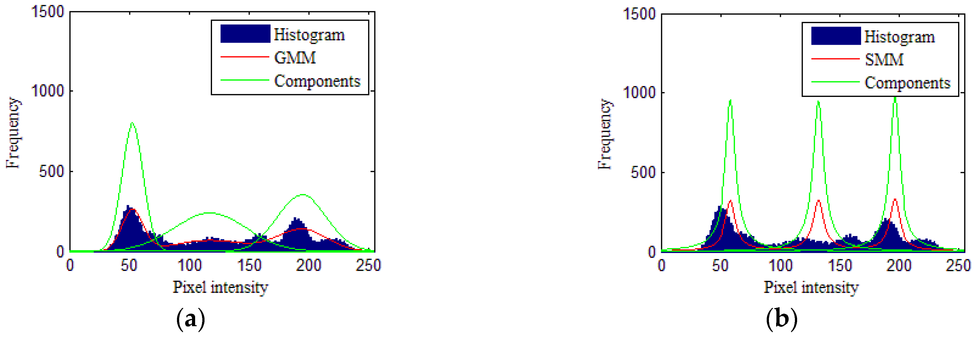
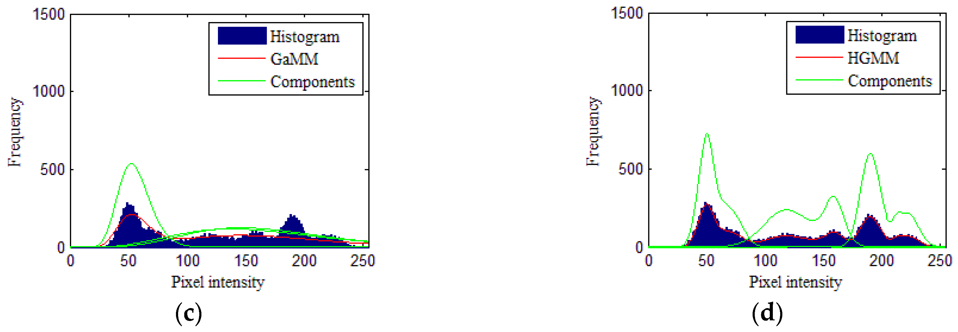
3.1. Simulated Image
3.2. High-Resolution Remote Sensing Image
4. Discussion
5. Conclusions
Author Contributions
Funding
Acknowledgments
Conflicts of Interest
References
- Lillesand, T.; Kiefer, R.W.; Chipman, J. Remote Sensing and Image Interpretation; John Wiley & Sons: Hoboken, NJ, USA, 2000. [Google Scholar]
- Zhang, X.L.; Xiao, P.F.; Feng, X.Z.; Wang, J.G.; Wang, Z. Hybrid region merging method for segmentation of high-resolution remote sensing images. ISPRS-J. Photogramm. Remote Sens. 2014, 98, 19–28. [Google Scholar] [CrossRef]
- Su, T.F.; Zhang, S.W. Local and global evaluation for remote sensing image segmentation. ISPRS-J. Photogramm. Remote Sens. 2017, 130, 256–276. [Google Scholar] [CrossRef]
- Grinias, I.; Panagiotakis, C.; Tziritas, G. MRF-based segmentation and unsupervised classification for building and road detection in peri-urban areas of high-resolution satellite images. ISPRS-J. Photogramm. Remote Sens. 2016, 122, 145–166. [Google Scholar] [CrossRef]
- Sang, Q.; Lin, Z.L.; Acton, S.T. Learning automata for image segmentation. Pattern Recognit. Lett. 2016, 74, 46–52. [Google Scholar] [CrossRef]
- Su, T.F. A novel region-merging approach guided by priority for high resolution image segmentation. Remote Sens. Lett. 2017, 8, 771–780. [Google Scholar] [CrossRef]
- Lei, T.; Xue, D.H.; Lv, Z.Y.; Li, S.Y.; Zhang, Y.N.; Asoke, K.N. Unsupervised change detection using fast fuzzy clustering for landslide mapping from very high-resolution images. Remote Sens. 2018, 10, 1381. [Google Scholar] [CrossRef]
- Nguyen, T.M.; Wu, Q.M.J. Fast and robust spatially constrained Gaussian mixture model for image segmentation. IEEE Trans. Circuits Syst. Video Technol. 2013, 23, 621–635. [Google Scholar] [CrossRef]
- Li, S.Z. Markov Random Field Modeling in Image Analysis; Springer Science & Business Media: New York, NY, USA, 2009. [Google Scholar]
- Mignotte, M. A label field fusion Bayesian model and its penalized maximum rand estimator for image segmentation. IEEE Trans. Image Process. 2010, 19, 1610–1624. [Google Scholar] [CrossRef]
- Song, S.; Si, B.; Herrmann, J.M.; Feng, X.S. Local autoencoding for parameter estimation in a hidden Potts-Markov random field. IEEE Trans. Image Process. 2016, 25, 324–2336. [Google Scholar] [CrossRef]
- Bouveyron, C.; Brunet-Saumard, C. Model-based clustering of high-dimensional data: A review. Comput. Stat. Data Anal. 2014, 71, 52–78. [Google Scholar] [CrossRef]
- Gómez-Chova, L.; Tuia, D.; Moser, G.; Camps-Valls, G. Multimodal classification of remote sensing images: A review and future directions. Proc. IEEE 2015, 103, 1–25. [Google Scholar] [CrossRef]
- Titterington, D.M.; Smith, A.F.M.; Markov, U.E. Statistical Analysis of Finite Mixture Distributions; Wiley: Hoboken, NJ, USA, 1985. [Google Scholar]
- Wang, Y.; Li, Y.; Zhao, Q.H. Segmentation of high-resolution SAR image with unknown number of classes based on regular tessellation and RJMCMC algorithm. Int. J. Remote Sens. 2015, 36, 1290–1306. [Google Scholar] [CrossRef]
- Mclachlan, G.J.; Peel, D. Finite Mixture Models; John Wiley & Sons: New York, NY, USA, 2000. [Google Scholar]
- Permuter, H.; Francos, J.; Jermyn, I. A study of Gaussian mixture models of color and texture features for image classification and segmentation. Pattern Recognit. 2006, 39, 695–706. [Google Scholar] [CrossRef]
- Nikou, C.; Galatsanos, N.P.; Likas, A.C. A class-adaptive spatially variant mixture model for image segmentation. IEEE Trans. Image Process. 2007, 16, 1121–1130. [Google Scholar] [CrossRef] [PubMed]
- Zhang, Y.; Brady, M.; Smith, S. Segmentation of brain MR images through a hidden Markov random field model and the expectation-maximization algorithm. IEEE Trans. Med. Imag. 2001, 20, 45–57. [Google Scholar] [CrossRef] [PubMed]
- Ji, Z.; Huang, Y.; Yong, X.; Zheng, Y. A robust modified Gaussian mixture model with rough set for image segmentation. Neurocomputing 2017, 266, 550–565. [Google Scholar] [CrossRef]
- Ban, Z.; Liu, J.; Li, C. Superpixel segmentation using Gaussian mixture model. IEEE Trans. Image Process. 2018, 27, 4105–4117. [Google Scholar] [CrossRef]
- Nguyen, T.M.; Wu, Q.M.J. Robust Student’ s-t mixture model with spatial constraints and its application in medical image segmentation. IEEE Trans. Med. Imag. 2012, 31, 103–116. [Google Scholar] [CrossRef]
- Gao, G.; Wen, C.; Wang, H. Fast and robust image segmentation with active contours and Student’s-t mixture model. Pattern Recognit. 2017, 63, 71–86. [Google Scholar] [CrossRef]
- Ziou, D.; Bouguila, N.; Allili, M.S.; El-Zaart, A. Finite gamma mixture modelling using minimum message length inference: Application to SAR image analysis. Int. J. Remote Sens. 2009, 30, 771–792. [Google Scholar] [CrossRef]
- Zhao, Q.H.; Li, X.L.; Li, Y. Multilook SAR image segmentation with an unknown number of clusters using a Gamma mixture model and hierarchical clustering. Sensors 2017, 17, 1114. [Google Scholar] [CrossRef] [PubMed]
- Nguyen, T.M.; Wu, Q.M.J.; Mukherjee, D.; Zhang, H. Bounded asymmetric mixture model for medical image segmentation. In Proceedings of the IEEE International Conference on Acoustics, Speech and Signal Processing, Vancouver, BC, Canada, 26–31 May 2013; IEEE: New Jersey, NJ, USA, 2013. [Google Scholar]
- Nguyen, T.M.; Wu, Q.M.J.; Zhang, H. Asymmetric mixture model with simultaneous feature selection and model detection. IEEE Trans. Neural Netw. Learn. Syst. 2015, 26, 400–408. [Google Scholar] [CrossRef] [PubMed]
- Ji, Z.; Huang, Y.; Sun, Q.; Cao, G.; Zheng, Y. A rough set bounded spatially constrained asymmetric Gaussian mixture model for image segmentation. PLoS ONE 2017, 12, 697–708. [Google Scholar] [CrossRef] [PubMed]
- Comer, M.L.; Delp, E.J. The EM/MPM algorithm for segmentation of textured images: Analysis and further experimental results. IEEE Trans. Image Process. 2000, 9, 1731–1744. [Google Scholar] [CrossRef]
- Congdon, P. Bayesian Statistical Modelling. Biometrics 2007, 63, 976–977. [Google Scholar]
- Nguyen, T.M.; Wu, Q.M.J. Dirichlet Gaussian mixture model: Application to image segmentation. Image Vis. Comput. 2011, 29, 818–828. [Google Scholar] [CrossRef]
- Stephens, M. Bayesian analysis of mixture models with an unknown number of components-an alternative to reversible jump methods. Ann. Stat. 2000, 28, 40–74. [Google Scholar] [CrossRef]
- Chatzis, S.P.; Varvarigou, T.A. A fuzzy clustering approach toward hidden Markov random field models for enhanced spatially constrained image segmentation. IEEE Trans. Fuzzy Syst. 2008, 16, 1351–1361. [Google Scholar] [CrossRef]


| Input: total iteration T, error e, k, δ, εμ, εσ, λ, μμ, σμ, μσ, σσ and β |
| Output: ci |
| Initialize Ψ(t), and t = 0 |
| While |log p(z|Ψ(t+1)) − log p(z|Ψ(t))| > e and t < T |
| Select α*, calculate a(α, α*) using Equation (15) |
| If a(α, α*) = 1 |
| α(t+1) = α* |
| Else |
| α(t+1) = α(t) |
| End if |
| Select w*, calculate a(w, w*) using Equation (17) |
| If a(w, w*) = 1 |
| w(t+1) = w* |
| Else |
| w(t+1) = w(t) |
| End if |
| Select θ*, calculate a(θ, θ*) using Equation (18) |
| If a(θ, θ*) = 1 |
| θ(t+1) = θ* |
| Else |
| θ(t+1) = θ(t) |
| End if |
| Generate r∈(0, 1) |
| If r > 0.5 |
| ml* = ml + 1 |
| Calculate R using Equation (20) |
| Calculate a(m, m*) = min(1, R) |
| Else |
| ml* = ml − 1 |
| Calculate R using Equation (20) |
| Calculate a(m, m*) = min(1, 1/R) |
| End if |
| If a(m, m*) = 1 |
| m(t+1) = m* |
| Else |
| m(t+1) = m(t) |
| End if |
| Calculate p(z|Ψ(t+1)) using Equation (6) |
| Calculate ci using Equation (22) |
| t = t + 1; |
| End while |
| T | e | δ | εμ | εσ | β | λ | μμ | σμ | μσ | σσ |
|---|---|---|---|---|---|---|---|---|---|---|
| 300,000 | 0.001 | 10 | 0.5 | 0.5 | 0.8 | 3 | 128 | 64 | 32 | 16 |
| Element | Region 1 (l = 1) | Region 2 (l = 2) | Region 3 (l = 3) | |||
|---|---|---|---|---|---|---|
| j = 1 | j = 2 | j = 1 | j = 2 | j = 1 | j = 2 | |
| wlj | 0.4 | 0.6 | 0.4 | 0.6 | 0.4 | 0.6 |
| μlj | 50 | 70 | 120 | 160 | 190 | 220 |
| σlj | 7 | 10 | 20 | 9 | 8 | 10 |
| Algorithm | Accuracy | Region 1 | Region 2 | Region 3 |
|---|---|---|---|---|
| HMRF algorithm | Users | 97.41 | 96.62 | 99.97 |
| Product | 98.87 | 96.67 | 98.21 | |
| Overall | 98.00 | |||
| Kappa | 0.97 | |||
| FCM algorithm | Users | 68.57 | 28.48 | 99.64 |
| Product | 55.81 | 43.11 | 95.34 | |
| Overall | 66.61 | |||
| Kappa | 0.56 | |||
| Gamma distribution-based algorithm | Users | 88.37 | 51.13 | 99.83 |
| Product | 99.72 | 77.92 | 68.72 | |
| Overall | 80.95 | |||
| Kappa | 0.73 | |||
| GMM algorithm | Users | 84.44 | 76.50 | 99.95 |
| Product | 99.34 | 79.41 | 82.56 | |
| Overall | 87.07 | |||
| Kappa | 0.81 | |||
| SMM algorithm | Users | 99.91 | 76.50 | 99.97 |
| Product | 93.29 | 99.81 | 88.25 | |
| Overall | 92.94 | |||
| Kappa | 0.89 | |||
| GaMM algorithm | Users | 98.02 | 32.91 | 100 |
| Product | 97.96 | 92.89 | 62.59 | |
| Overall | 79.23 | |||
| Kappa | 0.71 | |||
| HGMM algorithm | Users | 99.78 | 99.52 | 99.63 |
| Product | 99.78 | 99.54 | 99.60 | |
| Overall | 99.64 | |||
| Kappa | 0.99 | |||
| Algorithm | Overall Accuracy (%) | |||||
|---|---|---|---|---|---|---|
| Image 1 | Image 2 | Image 3 | Image 4 | Image 5 | Image 6 | |
| HMRF | 92.23 | 86.10 | 86.40 | 86.60 | 85.72 | 88.19 |
| FCM | 53.61 | 74.16 | 75.34 | 76.05 | 85.67 | 86.08 |
| Gamma | 62.82 | 87.30 | 59.61 | 64.57 | 66.88 | 62.84 |
| GMM | 82.04 | 88.49 | 85.49 | 84.92 | 82.56 | 85.59 |
| SMM | 75.89 | 66.06 | 69.81 | 88.28 | 68.43 | 78.56 |
| GaMM | 82.22 | 82.86 | 81.14 | 71.83 | 69.23 | 57.51 |
| HGMM | 95.43 | 96.28 | 90.44 | 93.48 | 88.90 | 88.94 |
| Algorithm | Times (Seconds) | |||||
|---|---|---|---|---|---|---|
| Image 1 | Image 2 | Image 3 | Image 4 | Image 5 | Image 6 | |
| HMRF | 74 | 76 | 86 | 85 | 98 | 96 |
| FCM | 63 | 71 | 89 | 99 | 108 | 124 |
| Gamma | 721 | 745 | 770 | 3012 | 29976 | 3060 |
| GMM | 134 | 116 | 148 | 364 | 463 | 494 |
| SMM | 238 | 275 | 388 | 895 | 1218 | 1523 |
| GaMM | 867 | 843 | 916 | 3286 | 3472 | 3646 |
| HGMM | 634 | 658 | 738 | 2245 | 2192 | 2375 |
© 2020 by the authors. Licensee MDPI, Basel, Switzerland. This article is an open access article distributed under the terms and conditions of the Creative Commons Attribution (CC BY) license (http://creativecommons.org/licenses/by/4.0/).
Share and Cite
Shi, X.; Li, Y.; Zhao, Q. Flexible Hierarchical Gaussian Mixture Model for High-Resolution Remote Sensing Image Segmentation. Remote Sens. 2020, 12, 1219. https://doi.org/10.3390/rs12071219
Shi X, Li Y, Zhao Q. Flexible Hierarchical Gaussian Mixture Model for High-Resolution Remote Sensing Image Segmentation. Remote Sensing. 2020; 12(7):1219. https://doi.org/10.3390/rs12071219
Chicago/Turabian StyleShi, Xue, Yu Li, and Quanhua Zhao. 2020. "Flexible Hierarchical Gaussian Mixture Model for High-Resolution Remote Sensing Image Segmentation" Remote Sensing 12, no. 7: 1219. https://doi.org/10.3390/rs12071219
APA StyleShi, X., Li, Y., & Zhao, Q. (2020). Flexible Hierarchical Gaussian Mixture Model for High-Resolution Remote Sensing Image Segmentation. Remote Sensing, 12(7), 1219. https://doi.org/10.3390/rs12071219