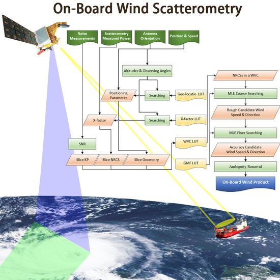
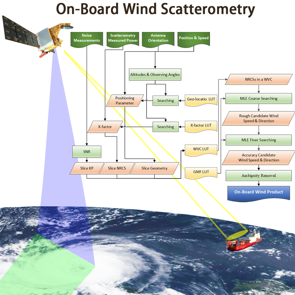
On-Board Wind Scatterometry


Abstract
1. Introduction
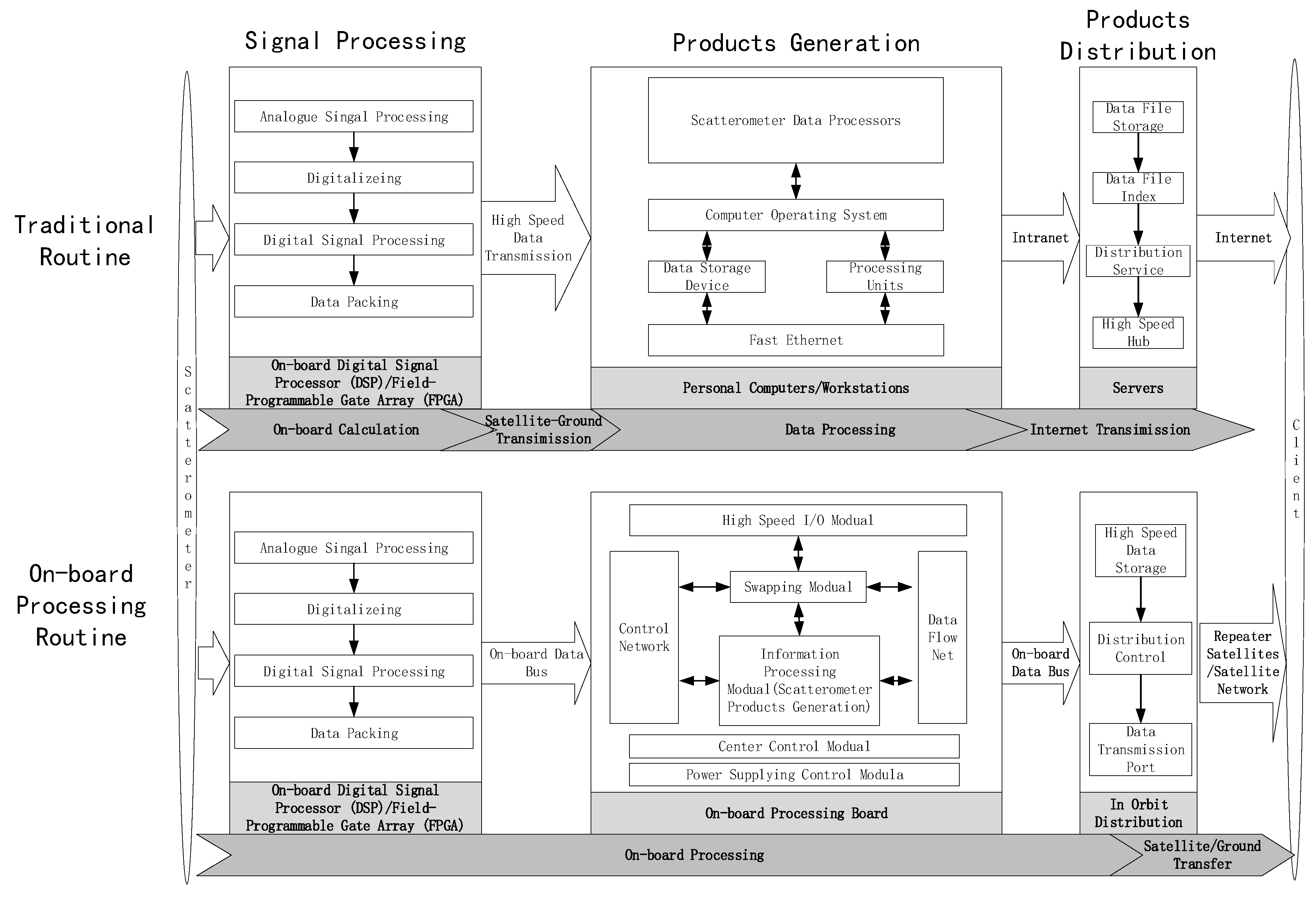
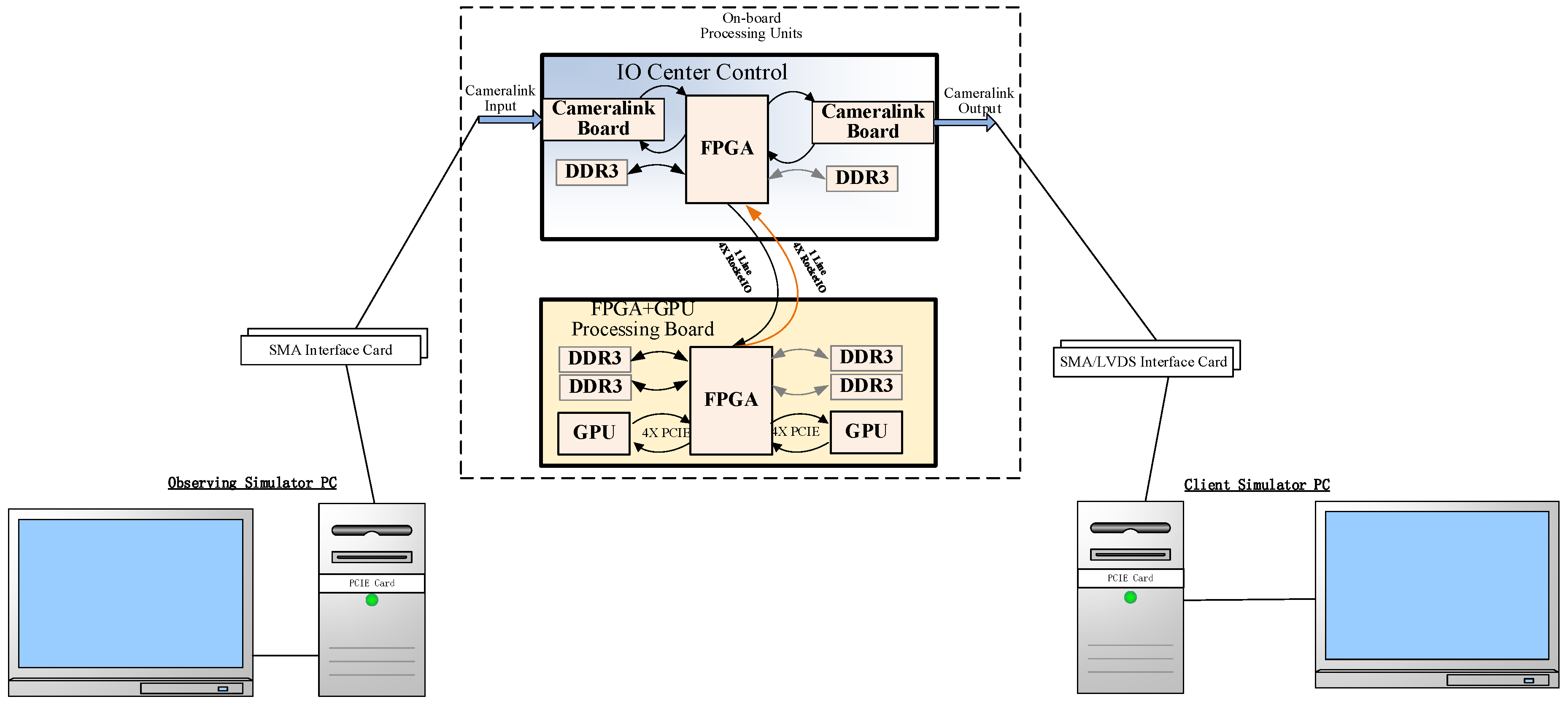
2. The On-Board Processing Environment and System
3. Wind Scatterometery Processing Chain and On-Board Processing Modifications
3.1. Modifications for On-Board Products
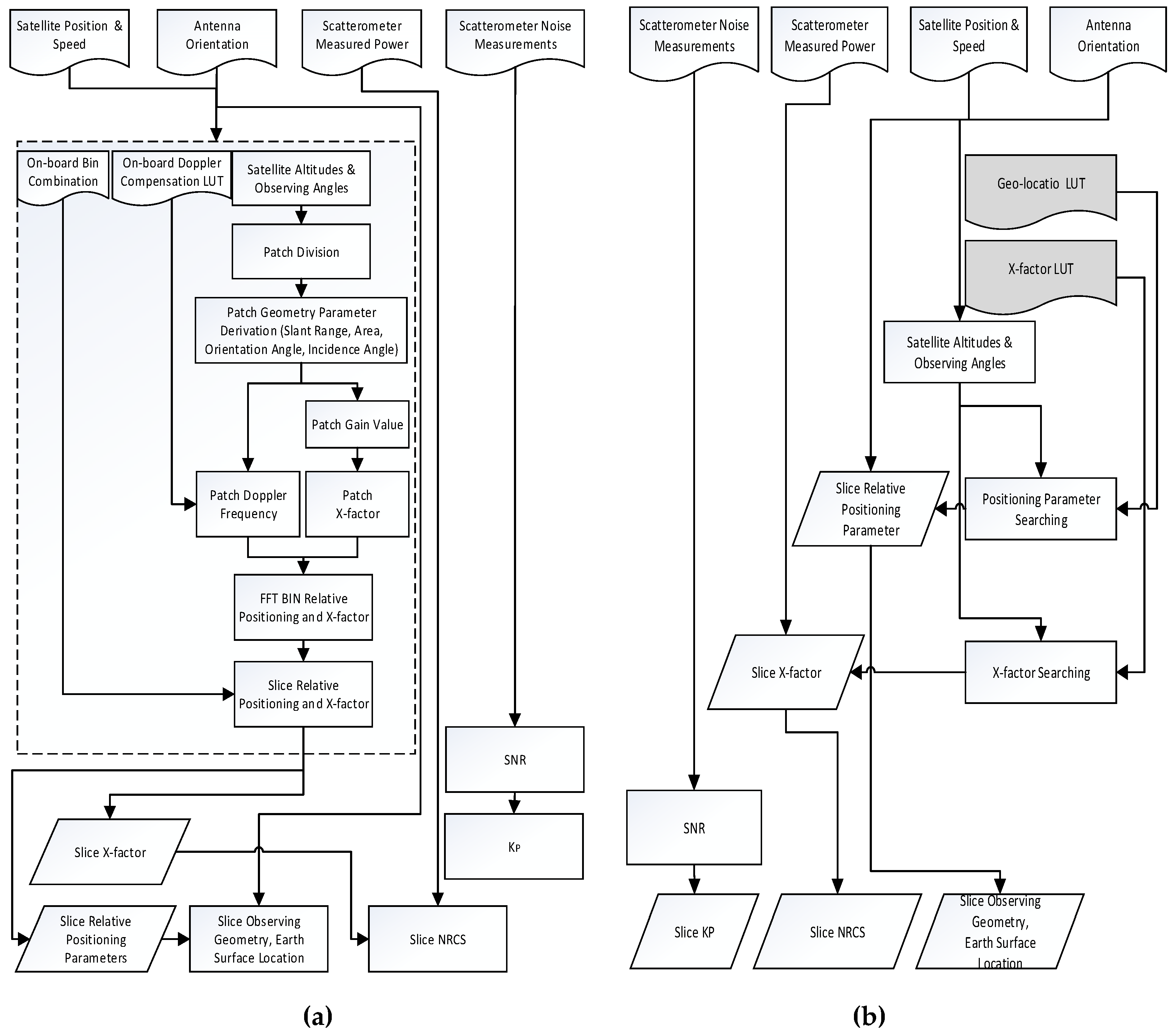
3.2. The On-Board Pre-Processing
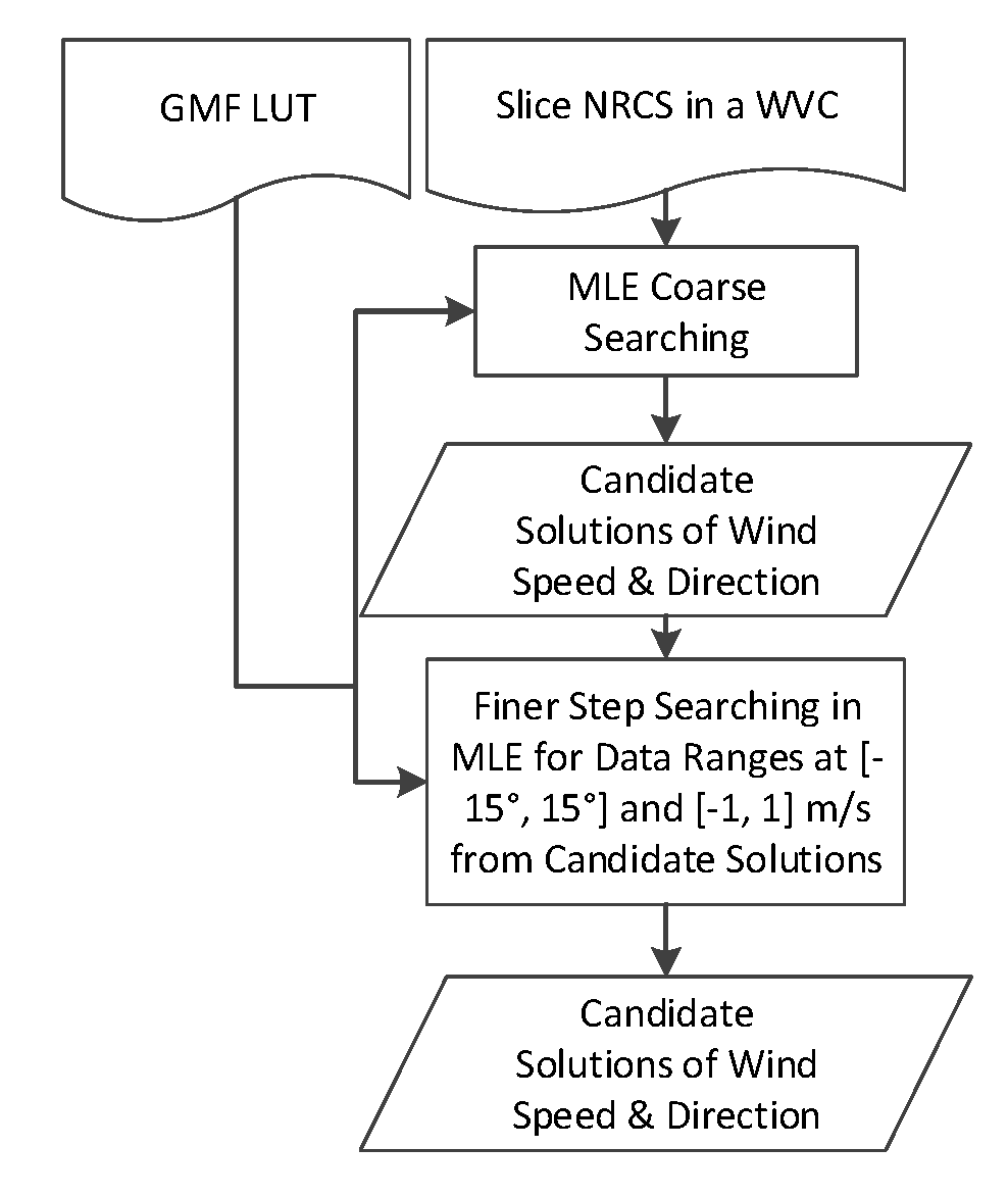
3.3. On-Board Wind Inversion
4. Experiment and Results
4.1. Data Description
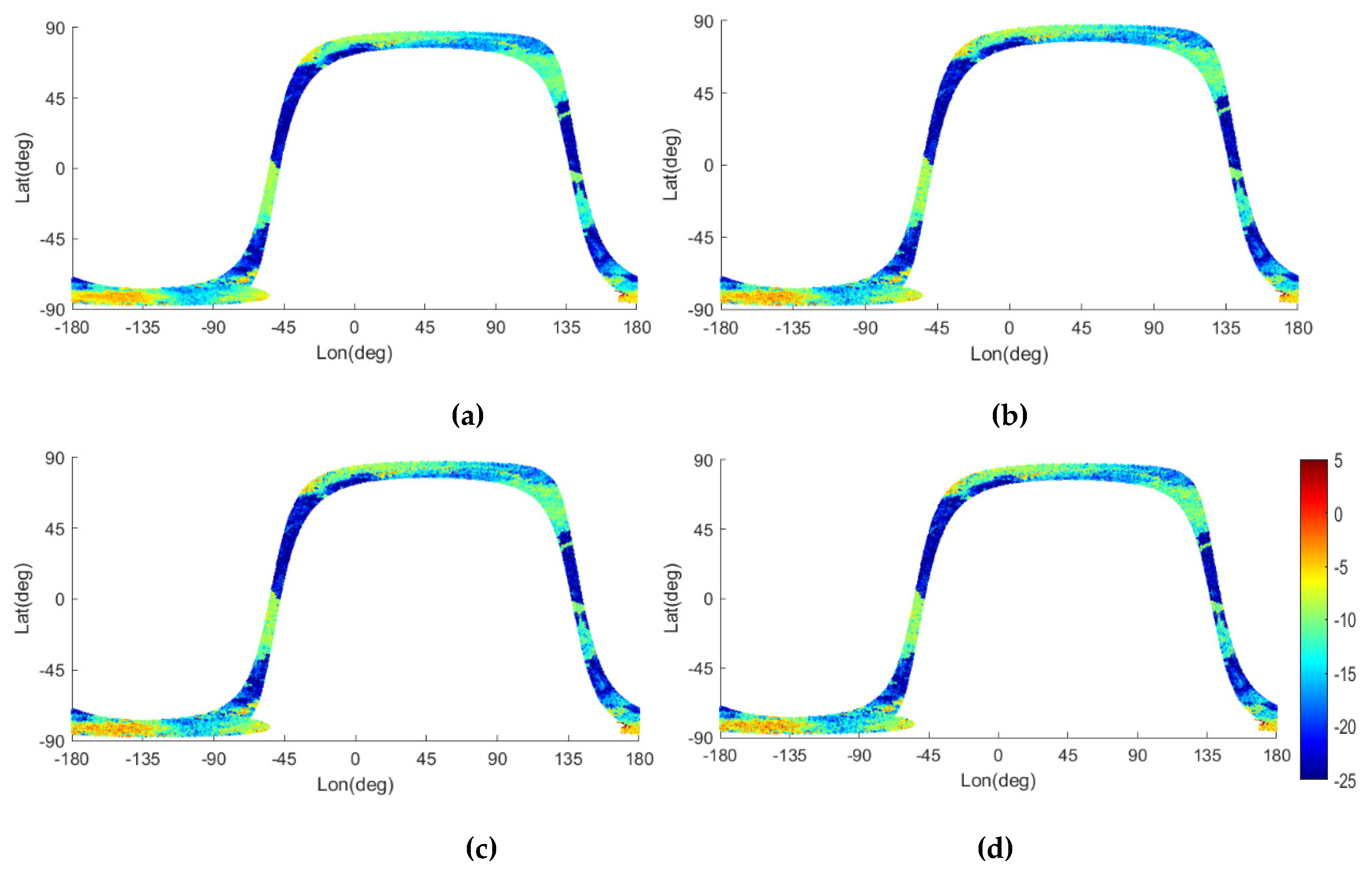
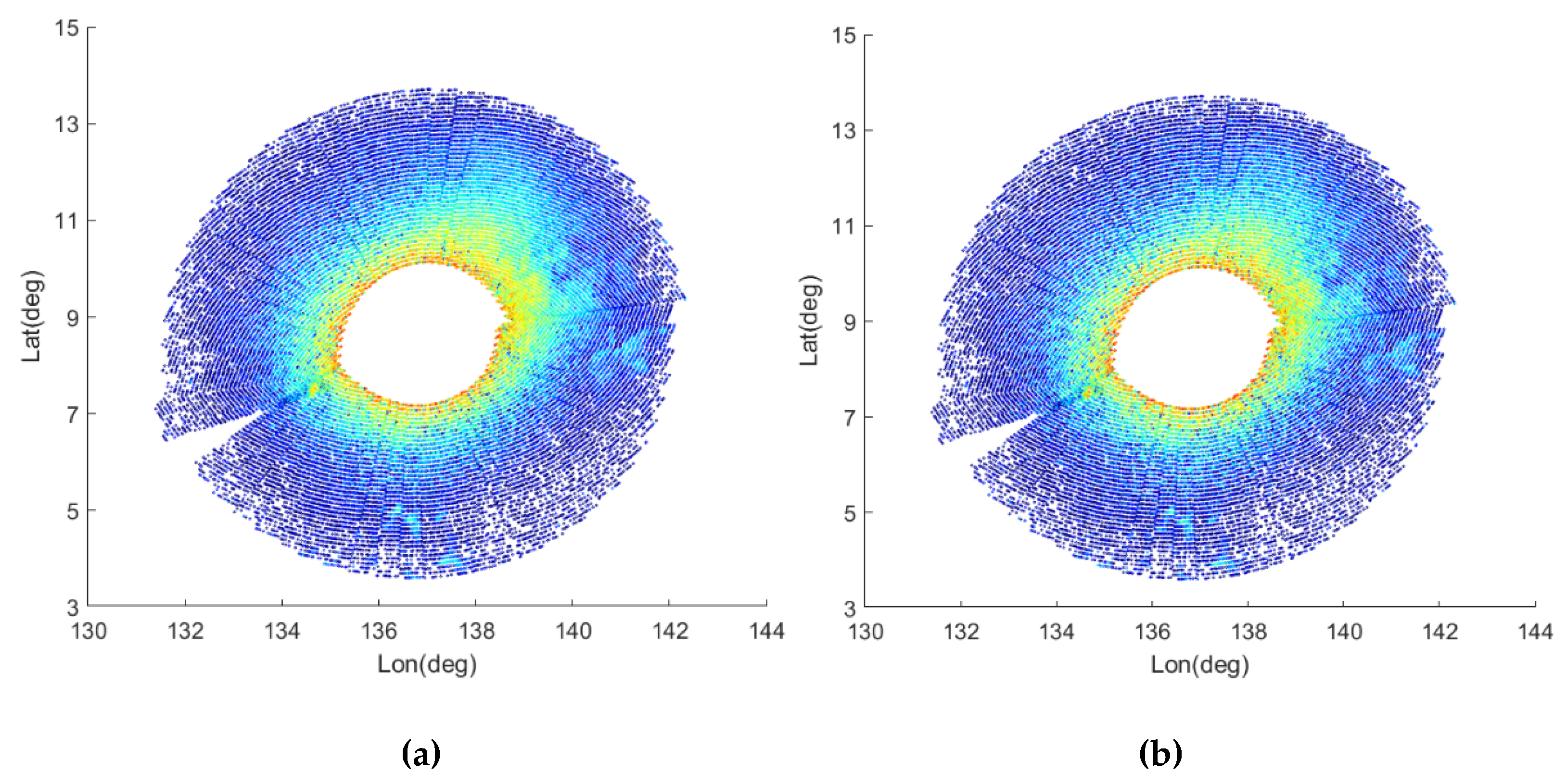
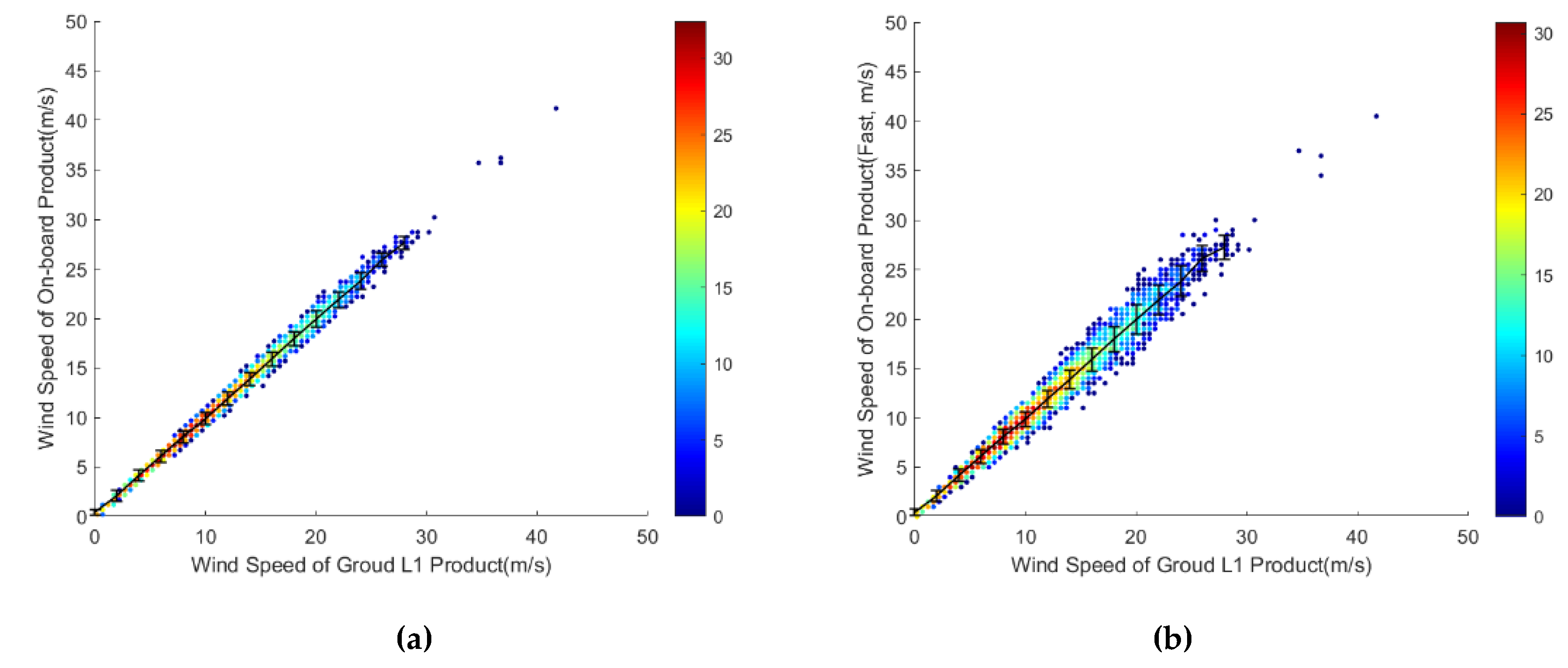
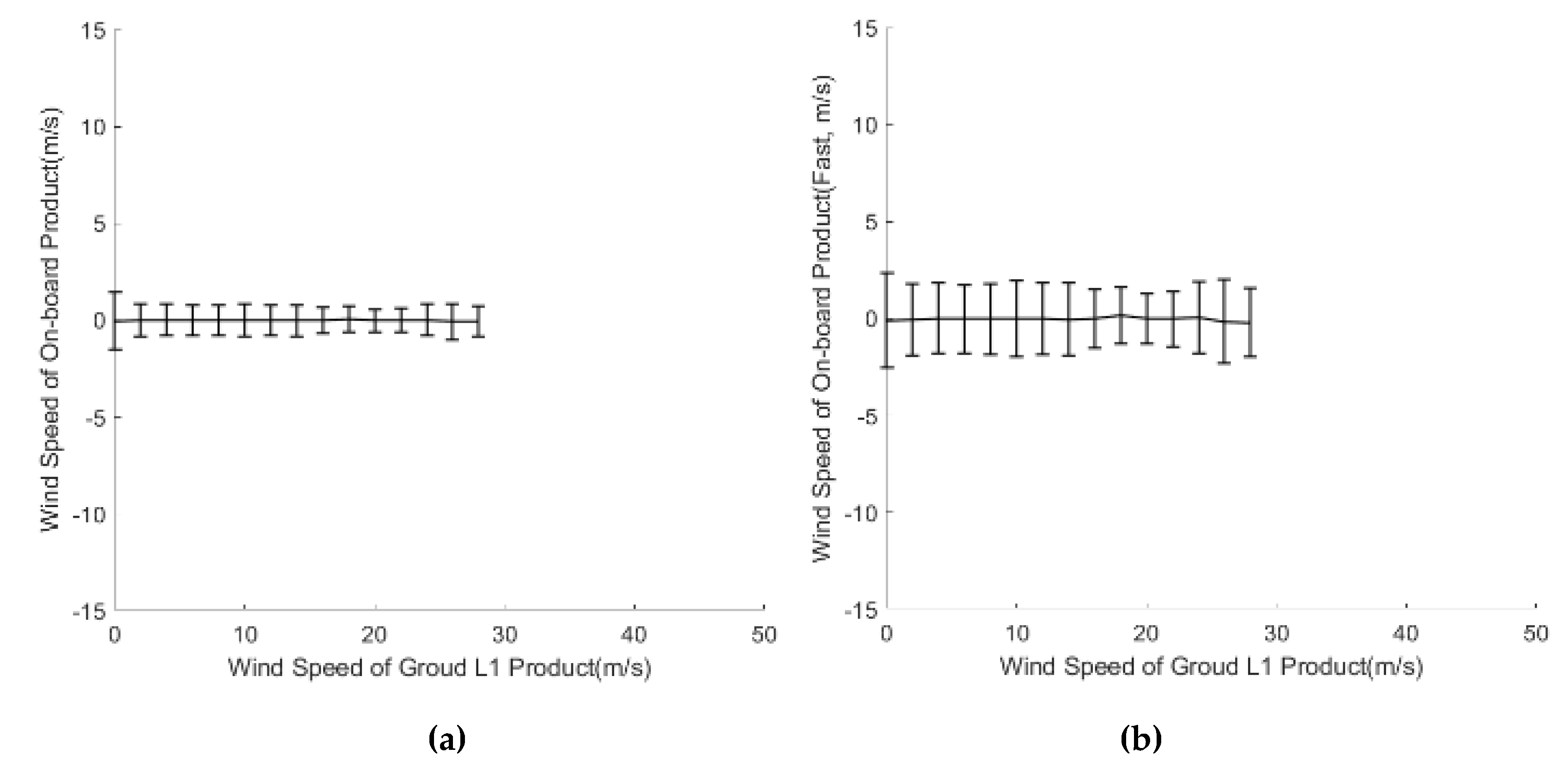
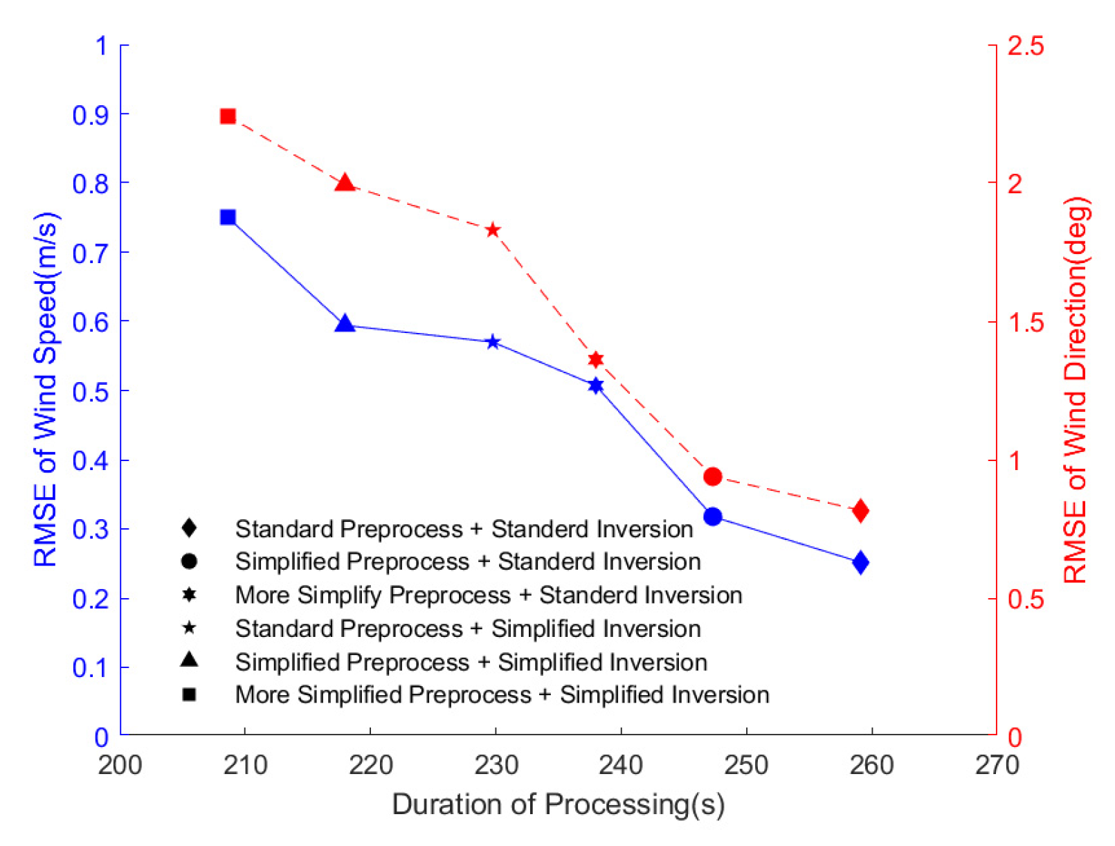
4.2. Results and Analysis
5. Summary and Discussion
Author Contributions
Funding
Acknowledgments
Conflicts of Interest
References
- Chang, P.S.; Jelenak, Z.; Sienkiewicz, J.; Knabb, R.; Brennan, M.; Long, D.G.; Freeberg, M. Operational Use and Impact of Satellite Remotely Sensed Ocean Surface Vector Winds in the Marine Warning and Forecasting Environment. Oceanography 2009, 22, 194–207. [Google Scholar] [CrossRef][Green Version]
- Stoffelen, A.; Kumar, R.; Zou, J.; Karaev, V.; Chang, P.S.; Rodriguez, E. Ocean Surface Vector Wind Observations. In Remote Sensing of the Asian Seas; Barale, V., Gade, M., Eds.; Springer: Cham, Switzerland, 2019; pp. 429–447. [Google Scholar]
- Benassai, G.; Migliaccio, M.; Montuori, A.; Ricchi, A. Wave Simulations Through Sar Cosmo-Skymed Wind Retrieval And Verification With Buoy Data. In Proceedings of the ISOPE-I-12-426, Rhodes, Greece, 17–22 June 2012; International Society of Offshore and Polar Engineers: Mountain View, CA, USA; p. 8.
- Montuori, A.; Ricchi, A.; Benassai, G.; Migliaccio, M. Sea Wave Numerical Simulations and Verification in Tyrrhenian Coastal Area with X-Band Cosmo-Skymed SAR Data; European Space Agency, (Special Publication) ESA SP: Paris, France, 2011; Volume 703, p. 17. [Google Scholar]
- Lin, C.-C.; Betto, M.; Rivas, M.B.; Stoffelen, A.; De Kloe, J. EPS-SG Windscatterometer Concept Tradeoffs and Wind Retrieval Performance Assessment. IEEE Trans. Geosci. Remote Sens. 2012, 50, 2458–2472. [Google Scholar] [CrossRef]
- Stoffelen, A. Scatterometry. Ph.D. Thesis, Universiteit Utrecht, Utrecht, The Netherlands, 1996. [Google Scholar]
- Stoffelen, A.; Verspeek, J.A.; Vogelzang, J.; Verhoef, A. The CMOD7 Geophysical Model Function for ASCAT and ERS Wind Retrievals. IEEE J. Sel. Top. Appl. Earth Obs. Remote Sens. 2017, 10, 1–12. [Google Scholar] [CrossRef]
- OSI SAF. Algorithm Theoretical Basis Document for the OSI SAF wind products and NSCAT-4 Geophysical Model Function. Available online: http://projects.knmi.nl/scatterometer/nscat_gmf/ (accessed on 22 July 2019).
- Verhoef, A.; Vogelzang, J.; Stoffelen, A. ASCAT L2 Winds Data Record Validation Report; Ocean and Sea Ice Satellite Application Facility, Eumetsat-Allee 1: Darmstadt, Germany; KNMI: De Bilt, The Netherlands, 2016. [Google Scholar]
- Verhoef, A.; Stoffelen, A. ASCAT Wind Validation Report; Ocean and Sea Ice Satellite Application Facility; KNMI: De Bilt, The Netherlands, 2018. [Google Scholar]
- Stoffelen, A.; Marseille, G. High Resolution Data Assimilation Guide; EUMETSAT: Darmstadt, Germany, 2018; Available online: https://www.nwpsaf.eu/site/download/documentation/scatterometer/reports/High_Resolution_Data_Assimilation_Guide_1.2.pdf (accessed on 2 March 2020).
- EUMETSAT. ASCAT—EUMETSAT. Available online: https://www.eumetsat.int/website/home/Satellites/CurrentSatellites/Metop/MetopDesign/ASCAT/index.html/ (accessed on 2 March 2020).
- AVISO. China France CFOSAT satellite data available. Available online: https://www.aviso.altimetry.fr/no_cache/en/news/front-page-news/news-detail.html?tx_ttnews%5Btt_news%5D=2533/ (accessed on 2 March 2020).
- NSOAS. HY-2 Series: HY-2A & HY-2B. Available online: http://www.nsoas.org.cn/eng/column/146.html (accessed on 2 March 2020).
- eoPortal Directory. SCATSat-1—Satellite Missions. Available online: https://directory.eoportal.org/web/eoportal/satellite-missions/s/scatsat-1 (accessed on 2 March 2020).
- CEOS. Overview of Scatterometer Missions over Time (Years). Available online: http://ceos.org/ourwork/virtual-constellations/osvw/ (accessed on 2 March 2020).
- OSI SAF Winds Team. ScatSat-1 Wind Product User Manual Version 1.3; Ocean and Sea Ice Satellite Application Facility—Eumetsat-Allee 1: Darmstadt, Germany; KNMI: De Bilt, The Netherlands, 2018; Available online: http://projects.knmi.nl/scatterometer/publications/pdf/osisaf_cdop2_ss3_pum_scatsat1_winds.pdf. (accessed on 2 March 2020).
- Stiles, B.; Pollard, B.; Dunbar, R. Direction interval retrieval with thresholded nudging: A method for improving the accuracy of QuikSCAT winds. IEEE Trans. Geosci. Remote Sens. 2002, 40, 79–89. [Google Scholar] [CrossRef]
- Fore, A.; Stiles, B.W.; Chau, A.H.; Williams, B.A.; Dunbar, R.S.; Rodriguez, E. Point-Wise Wind Retrieval and Ambiguity Removal Improvements for the QuikSCAT Climatological Data Set. IEEE Trans. Geosci. Remote Sens. 2014, 52, 51–59. [Google Scholar] [CrossRef]
- TD 14—EUMETSAT Advanced Retransmission Service Technical Description; EUMETSAT: Darmstadt, Germany, Eumetsat-Allee 1; 2019; Available online: https://www.eumetsat.int/website/wcm/idc/idcplg?IdcService=GET_FILE&dDocName=PDF_DMT_112370&RevisionSelectionMethod=LatestReleased&Rendition=Web (accessed on 2 March 2020).
- King, G.P.; Portabella, M.; Lin, W.; Stoffelen, A. Correlating Extremes in Wind and Stress Divergence with Extremes in Rain over the Tropical Atlantic; Ocean and Sea Ice SAF Scientific Report; KNMI: De Bilt, The Netherlands, 2017. [Google Scholar]
- Gehrig, S.K.; Eberli, F.; Meyer, T. A Real-Time Low-Power Stereo Vision Engine Using Semi-Global Matching. In Computer Vision Systems; Academic Press: Cambridge, MA, USA, 2009; Volume 5815, pp. 134–143. [Google Scholar]
- Qi, B.; Shi, H.; Zhuang, Y.; Chen, H.; Chen, L. On-Board, Real-Time Preprocessing System for Optical Remote-Sensing Imagery. Sensors 2018, 18, 1328. [Google Scholar] [CrossRef] [PubMed]
- Wohlfeil, J.; Börner, A.; Buder, M.; Ernst, I.; Krutz, D.; Reulke, R. REAL TIME DATA PROCESSING FOR OPTICAL REMOTE SENSING PAYLOADS. In Proceedings of the XXII ISPRS Congress, Melbourne, Australia, 5 August–1 September 2012; Volume XXXIX-B5, pp. 64–68. [Google Scholar]
- Lim, S.; Xiaofang, C. High performance on-board processing and storage for satellite remote sensing applications. In Proceedings of the 2014 IEEE International Conference on Aerospace Electronics and Remote Sensing Technology, Yogyakarta, Indonesia, 13–14 November 2014; pp. 137–141. [Google Scholar]
- Yao, Y.; Jiang, Z.; Zhang, H.; Zhou, Y. On-Board Ship Detection in Micro-Nano Satellite Based on Deep Learning and COTS Component. Remote Sens. 2019, 11, 762. [Google Scholar] [CrossRef]
- Foust, J. SpaceX’s space-Internet woes: Despite technical glitches, the company plans to launch the first of nearly 12,000 satellites in 2019. IEEE Spectr. 2019, 56, 50–51. [Google Scholar] [CrossRef]
- Xu, J.; Zhang, G. Design and Transmission Performance Analysis of Satellite Constellation for Broadband LEO Constellation Satellite Communication System Based On High Elevation Angle. IOP Conf. Ser.: Mater. Sci. Eng. 2018, 452, 042092. [Google Scholar] [CrossRef]
- Zhou, G.; Baysal, O.; Kaye, J.; Habib, S.; Wang, C. Concept design of future intelligent Earth observing satellites. Int. J. Remote Sens. 2004, 25, 2667–2685. [Google Scholar] [CrossRef]
- Li, D.; Wang, M.; Dong, Z.; Shen, X.; Shi, L. Earth observation brain (EOB): An intelligent earth observation system. Geo-spatial Inf. Sci. 2017, 20, 134–140. [Google Scholar] [CrossRef]
- Sevellec, F.; Drijfhout, S.S. A novel probabilistic forecast system predicting anomalously warm 2018-2022 reinforcing the long-term global warming trend. Nat. Commun. 2018, 9, 3024. [Google Scholar] [CrossRef] [PubMed]
- Skolnik, M.I. Radar Handbook, 3rd ed.; McGraw-Hill Education: New York, NY, USA, 2008; pp. 18–53. [Google Scholar]
- Woodhouse, I.H. Introduction to Microwave Remote Sensing; CRC Press: Boca Raton, FL, USA, 2005; p. 166. [Google Scholar]
- Dunbar, S.; Stiles, B.; Huddleston, J.; Callahan, H.; Lungu, T.; Mears, C.; Wentz, F.; Smith, D. SeaWinds Science Data Product User’s Manual Overview & Geophysical Data Products version 2; JPL: Pasadena, CA, USA, 2006. Available online: https://podaac-tools.jpl.nasa.gov/drive/files/allData/seawinds/L2BE/docs/SWS_SDPUG_V2.0.pdf (accessed on 2 March 2020).
- Nvidia, JETSON TX2. Available online: https://www.nvidia.cn/autonomous-machines/embedded-systems/jetson-tx2 (accessed on 2 March 2020).
- George, A.D.; Wilson, C.M. Onboard Processing With Hybrid and Reconfigurable Computing on Small Satellites. Proc. IEEE 2018, 106, 458–470. [Google Scholar] [CrossRef]
- Su, Y.; Liu, Y.; Zhou, Y.; Yuan, J.; Cao, H.; Shi, J. Broadband LEO Satellite Communications: Architectures and Key Technologies. IEEE Wirel. Commun. 2019, 26, 55–61. [Google Scholar] [CrossRef]
- Driesenaar, T.; de Kloe, J.; Stoffelen, A.; Forneris, V. PRODUCT USER MANUAL For Wind- Global Ocean L3 Wind; KNMI: De Bilt, The Netherlands, 2016; Available online: https://cdn.knmi.nl/system/data_center_publications/files/000/070/016/original/cmemsosipum012002.pdf?1495622122 (accessed on 2 March 2020).
- Freilich, M.H. SeaWinds ALGORITHM THEORETICAL BASIS DOCUMENT; NASA: Washington, DC, USA, 2012. Available online: https://eospso.nasa.gov/sites/default/files/atbd/atbd-sws-01.pdf (accessed on 2 March 2020).
- Spencer, M.W.; Wu, C.; Long, D.G. Improved resolution backscatter measurements with the SeaWinds pencil-beam scatterometer. IEEE Trans. Geosci. Remote Sens. 2000, 38, 89–104. [Google Scholar] [CrossRef]
- Xu, X.; Dong, X.; Zhu, D.; Lin, W. Pre-processing algorithm and airborne campaign result analysis of a rotating fan-beam scatterometer. In Proceedings of the SPIE Asia-Pacific Remote Sensing, Beijing, China, 13–17 October 2014; SPIE: Bellingham, WA, USA; Volume 9264. [Google Scholar]
- Vogelzang, J. Two Dimensional Variational Ambiguity Removal (2DVAR); KNMI: De Bilt, The Netherlands, 2017; Available online: http://citeseerx.ist.psu.edu/viewdoc/download;jsessionid=88BBD01BAD28915EE1C4869F66E91F73?doi=10.1.1.627.1963&rep=rep1&type=pdf (accessed on 2 March 2020).
- Lin, W.; Dong, X.; Portabella, M.; Lang, S.; He, Y.; Yun, R.; Wang, Z.; Xu, X.; Zhu, D.; Liu, J. A Perspective on the Performance of the CFOSAT Rotating Fan-Beam Scatterometer. IEEE Trans. Geosci. Remote Sens. 2018, 57, 627–639. [Google Scholar] [CrossRef]
- NSOAS. NSOAS Data Distribution. Available online: https://osdds.nsoas.org.cn (accessed on 22 January 2020).


| Indexes | |
|---|---|
| Weight | 15 kg |
| Size | 425 × 254 × 240 mm |
| Power | 280 W |
| Temperature | 50 °C |
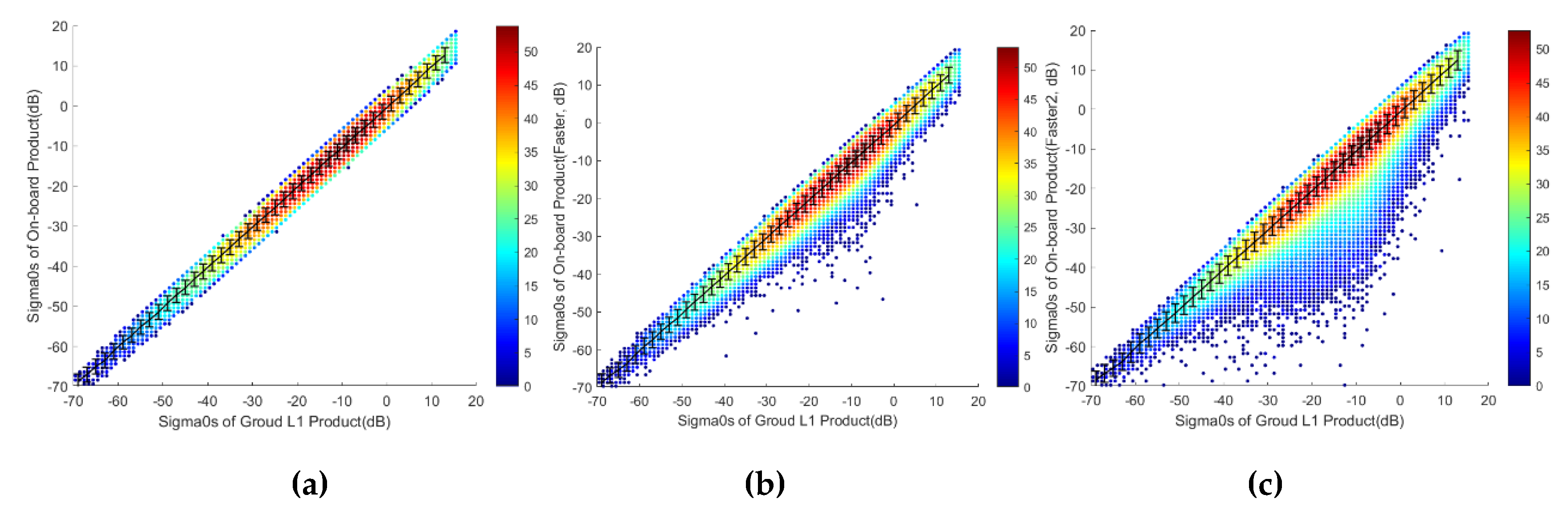
| Differences (dB) | Stdev.(dB) | |||||
|---|---|---|---|---|---|---|
| Mean | Maximum | Corresponding Normalized Radar Cross Section (NRCS) of Maximum | Mean | Maximum | Corresponding NRCS of Maximum | |
| Look-Up Tabls (LUTs) in original resolution | −0.28 | −0.53 | −63 | 1.83 | 1.94 | −61 |
| LUTs resampled in a half number | −0.41 | −0.72 | −63 | 2.06 | 2.3 | −61 |
| LUTs resampled in a quarter number | −0.52 | −0.82 | −63 | 2.2 | 2.57 | −61 |
© 2020 by the authors. Licensee MDPI, Basel, Switzerland. This article is an open access article distributed under the terms and conditions of the Creative Commons Attribution (CC BY) license (http://creativecommons.org/licenses/by/4.0/).
Share and Cite
Xu, X.; Dong, X.; Xie, Y. On-Board Wind Scatterometry. Remote Sens. 2020, 12, 1216. https://doi.org/10.3390/rs12071216
Xu X, Dong X, Xie Y. On-Board Wind Scatterometry. Remote Sensing. 2020; 12(7):1216. https://doi.org/10.3390/rs12071216
Chicago/Turabian StyleXu, Xingou, Xiaolong Dong, and Yu Xie. 2020. "On-Board Wind Scatterometry" Remote Sensing 12, no. 7: 1216. https://doi.org/10.3390/rs12071216
APA StyleXu, X., Dong, X., & Xie, Y. (2020). On-Board Wind Scatterometry. Remote Sensing, 12(7), 1216. https://doi.org/10.3390/rs12071216