Effects on the Double Bounce Detection in Urban Areas Based on SAR Polarimetric Characteristics

 and
and
Abstract
1. Introduction
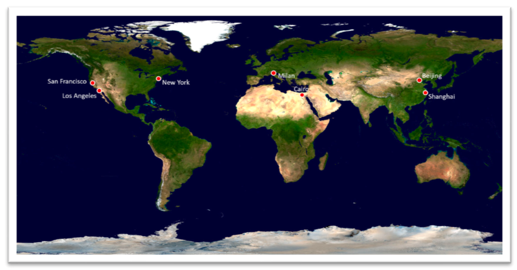
2. Study Areas
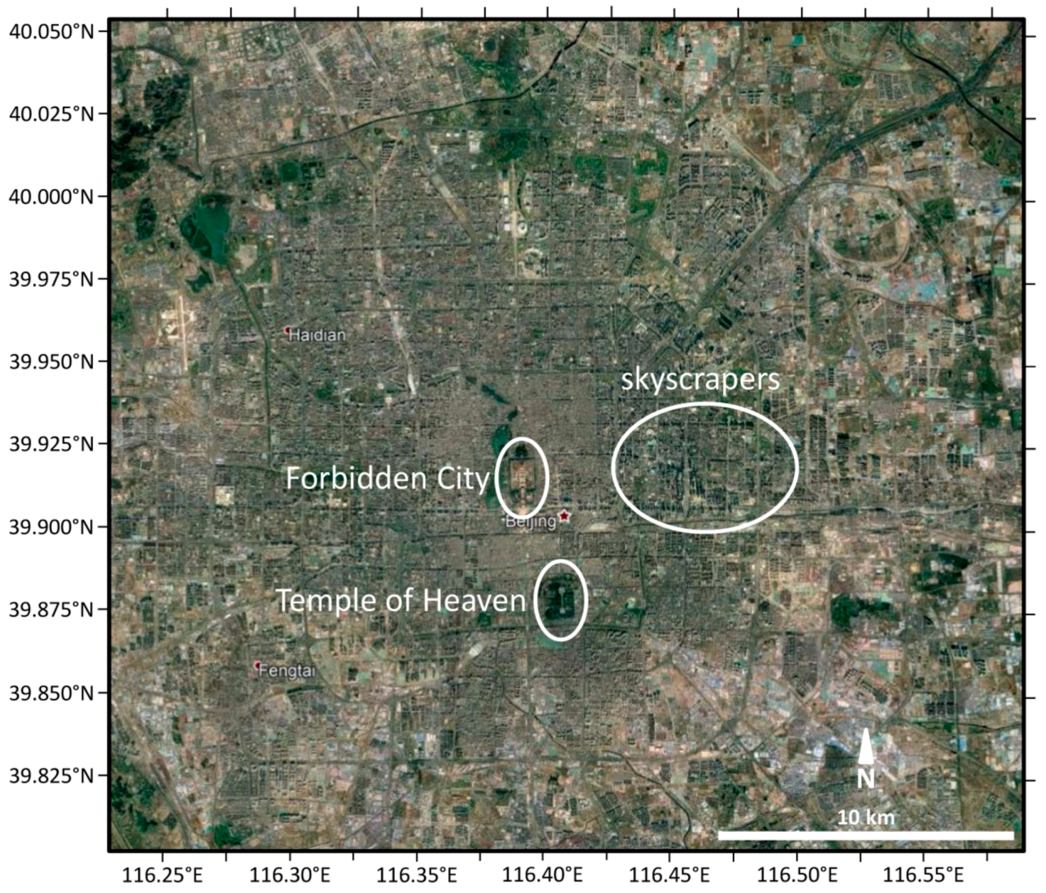
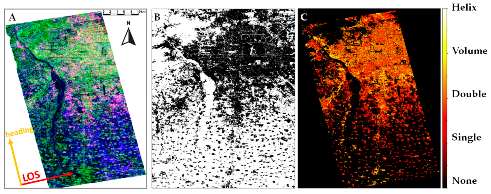
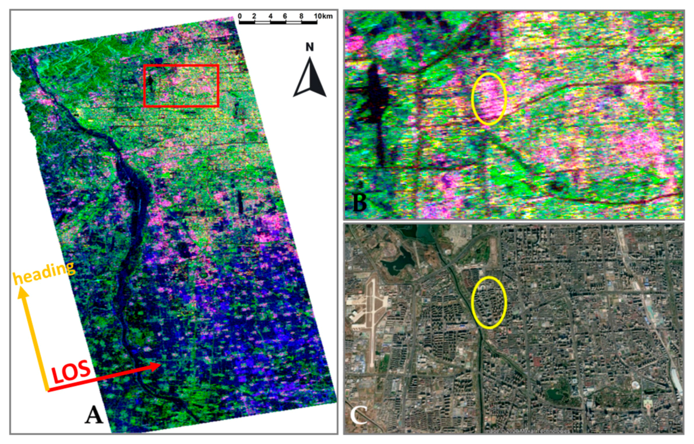
2.1. Beijing
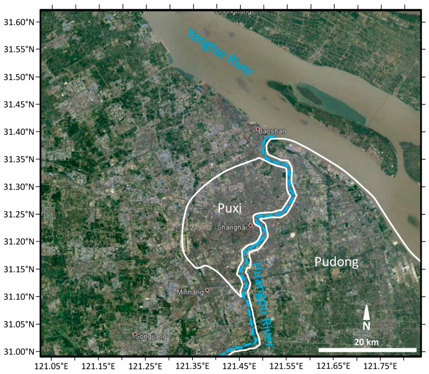
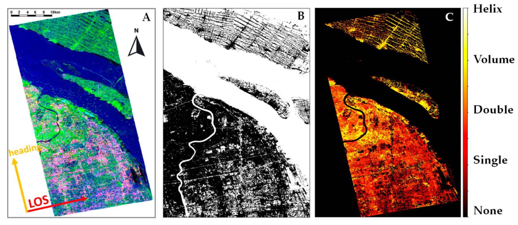
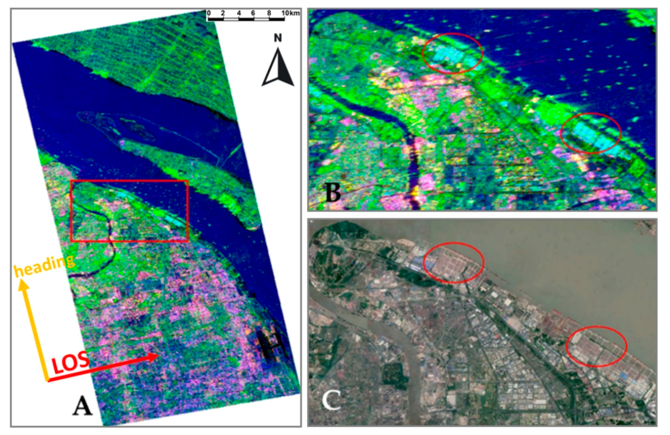
2.2. Shanghai
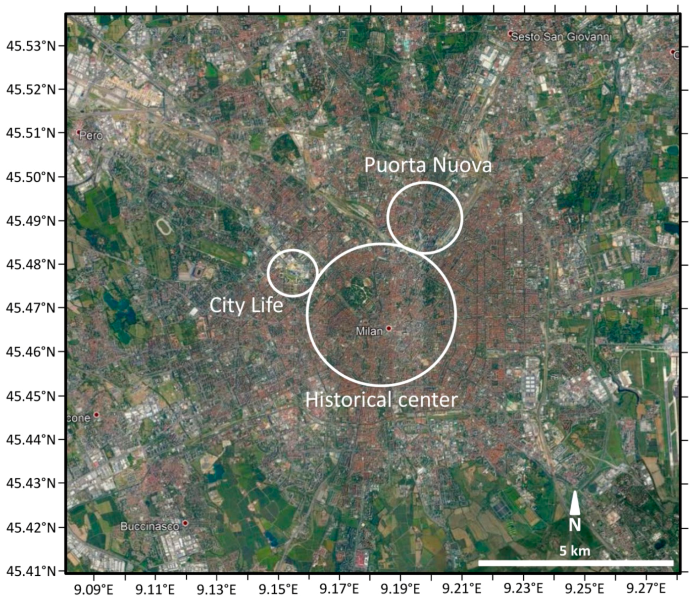
2.3. Milan
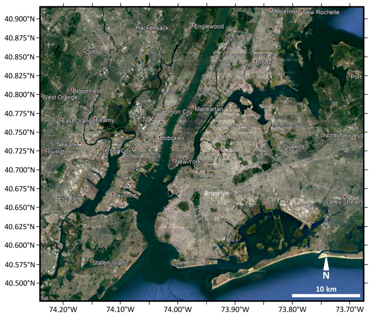
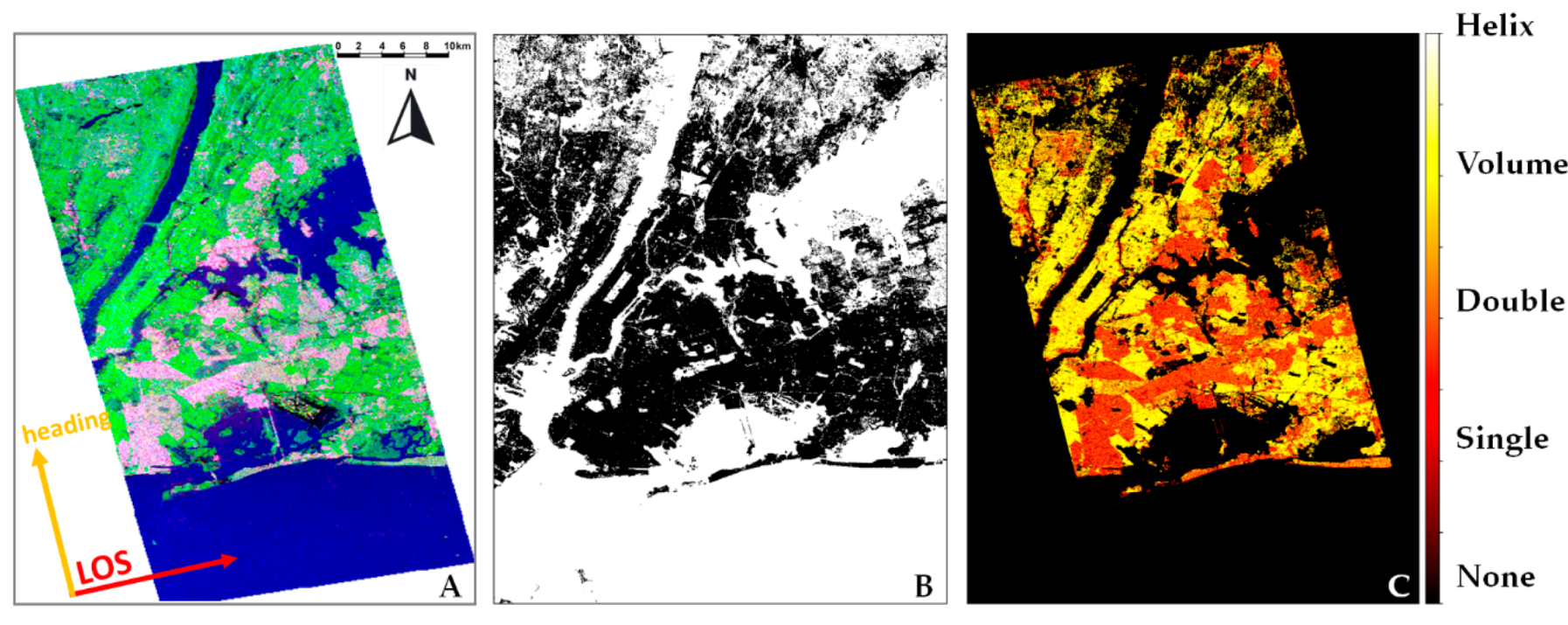
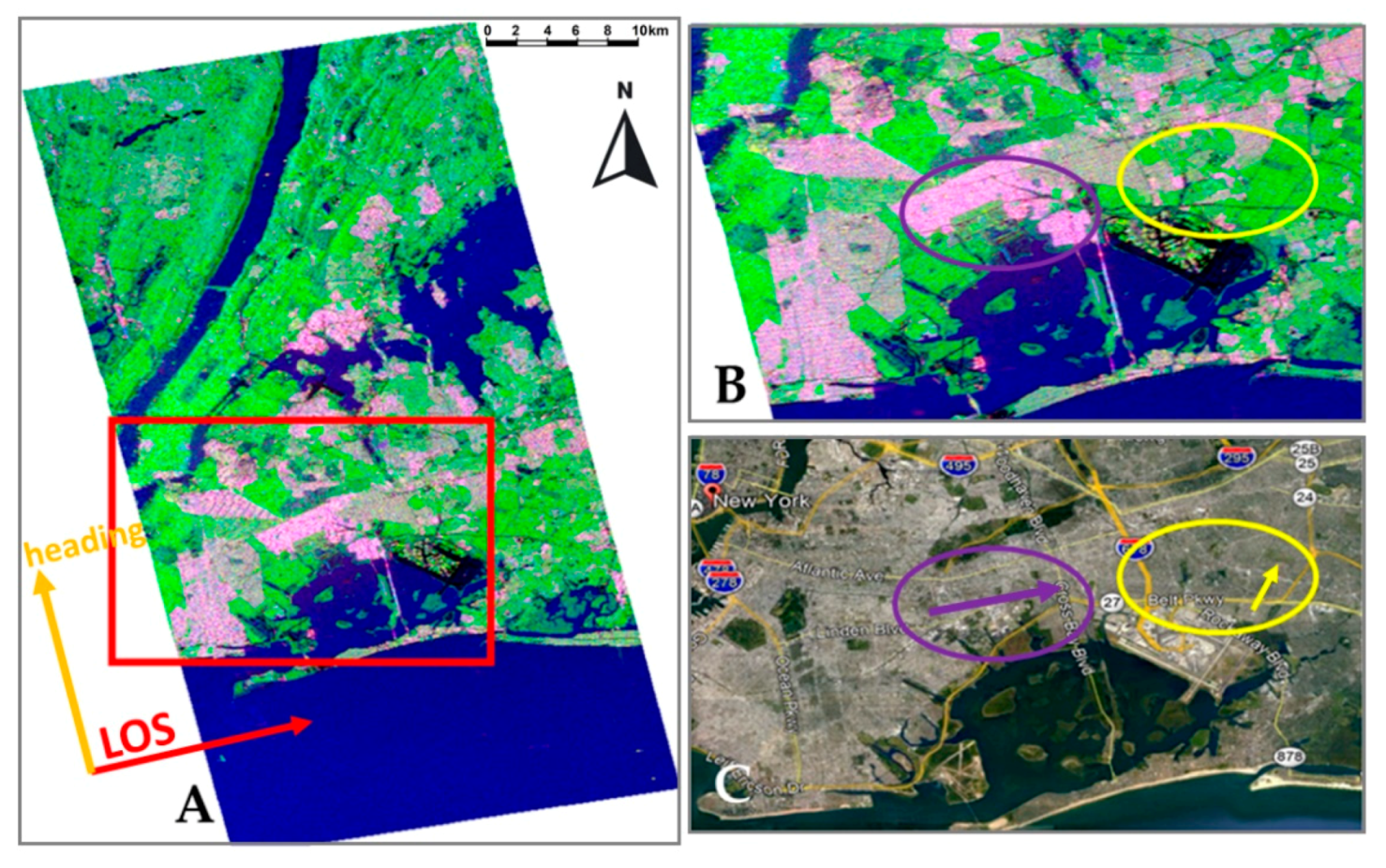
2.4. New York
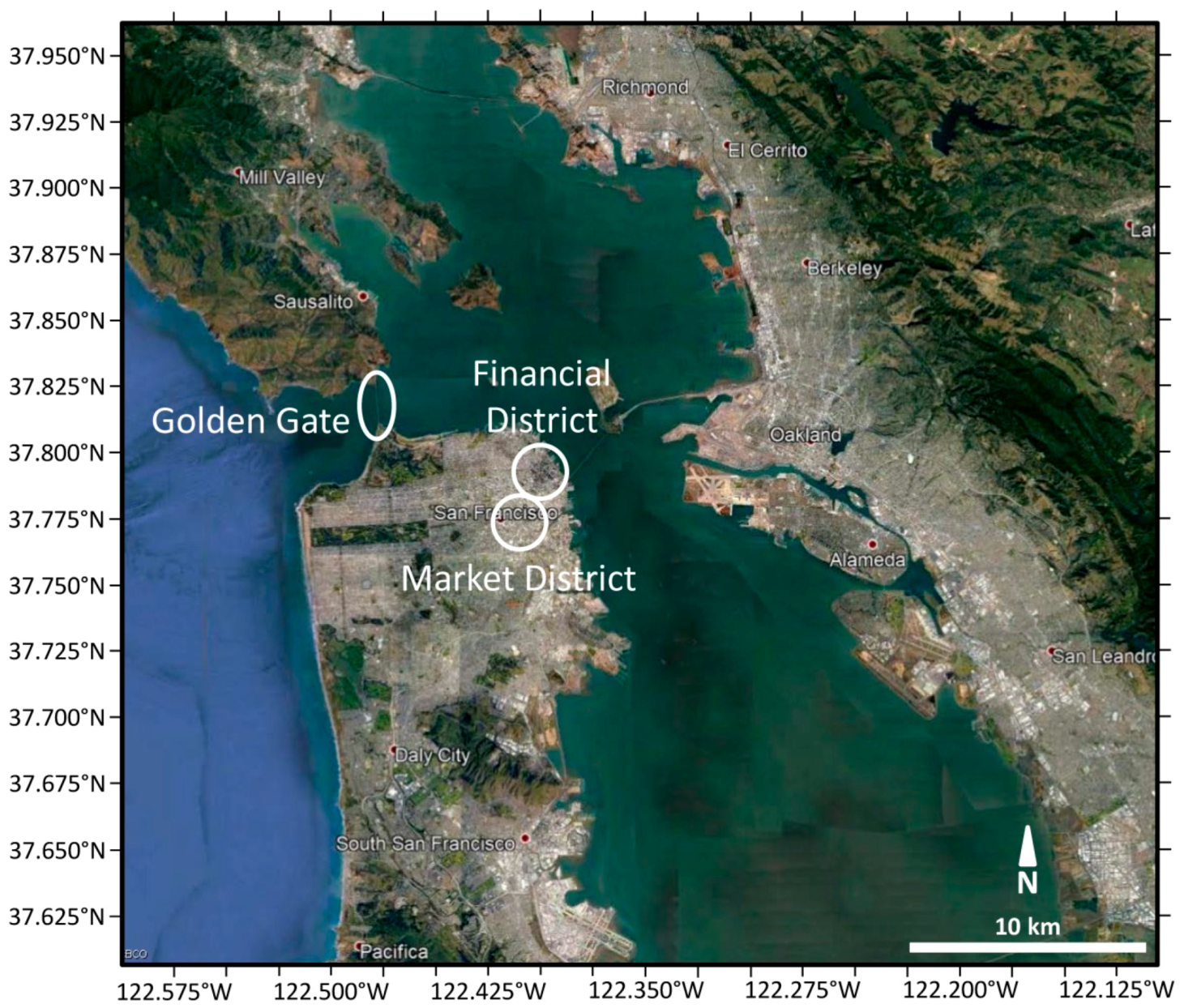
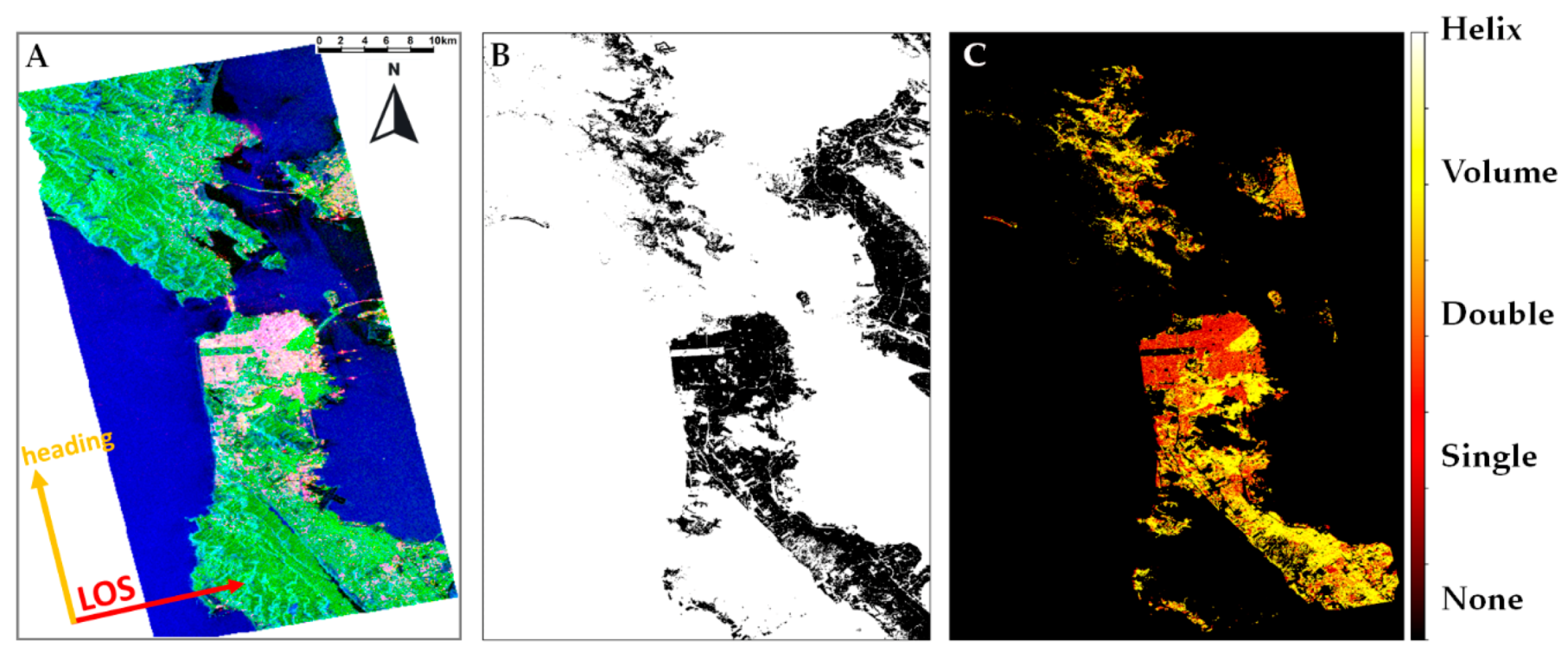
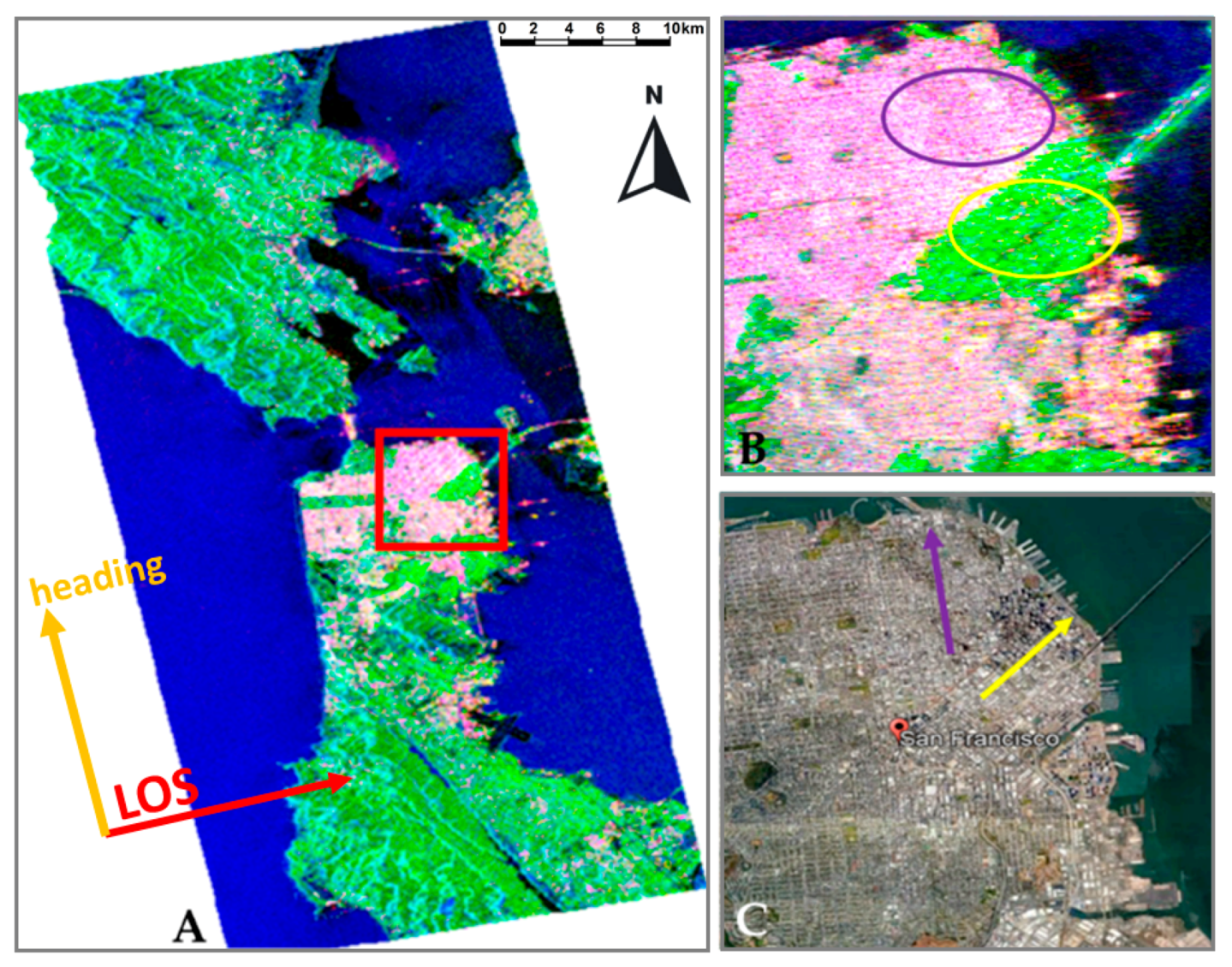
2.5. San Francisco
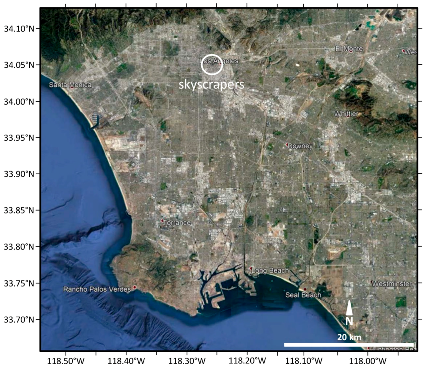
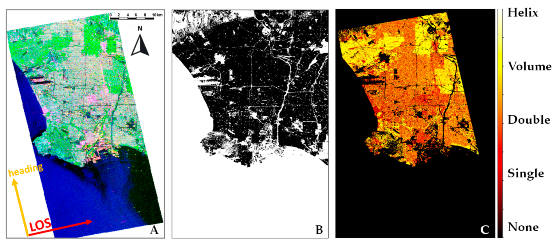
2.6. Los Angeles
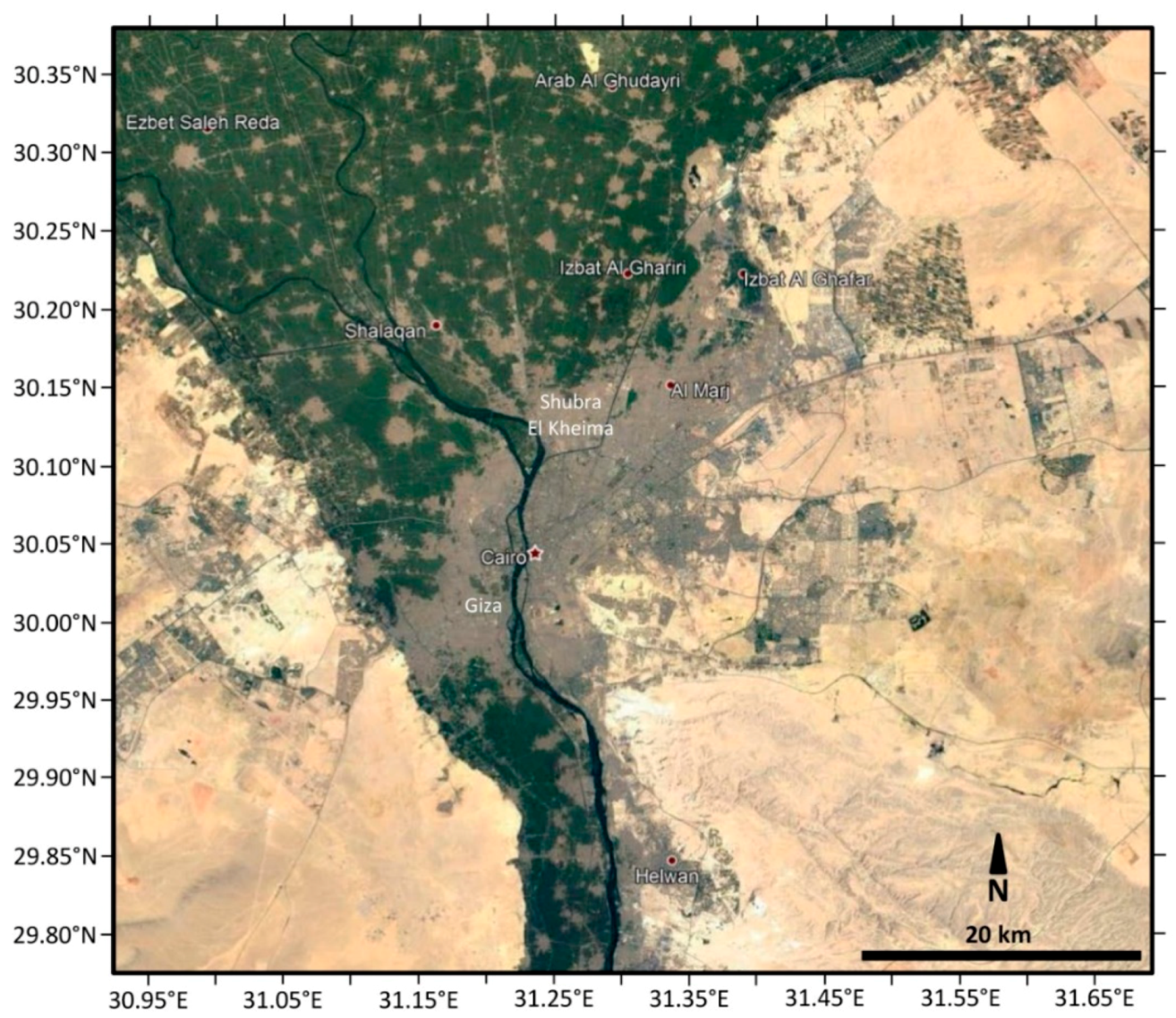
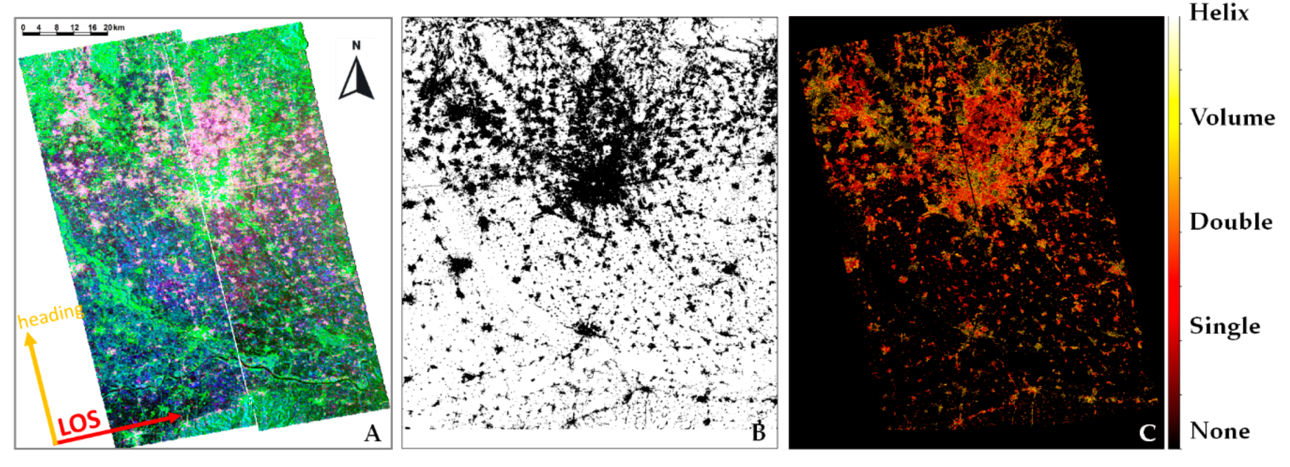
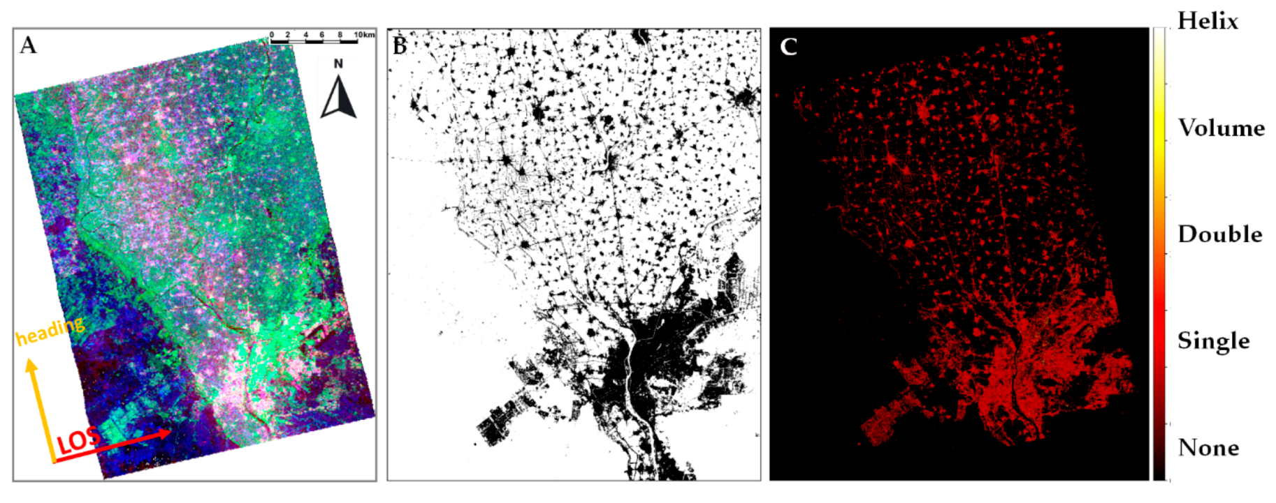
2.7. Greater Cairo
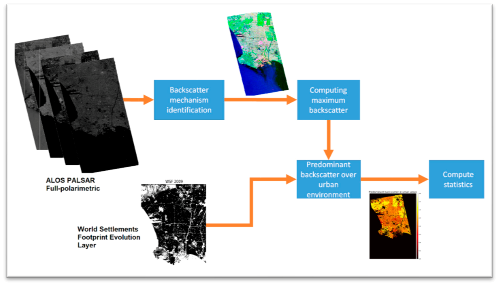
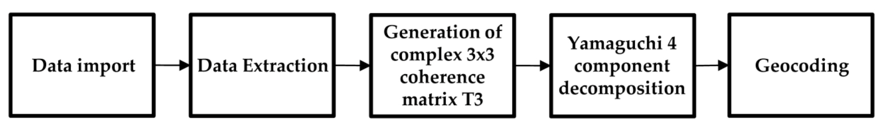
3. Dataset and Methods
4. Results
5. Discussion
6. Conclusions
Author Contributions
Funding
Acknowledgments
Conflicts of Interest
Appendix A


References
- Lee, J.-S.; Pottier, E. Polarimetric Radar Imaging: From Basics to Applications; CRC Press: Boca Raton, FL, USA, 2009. [Google Scholar]
- Patruno, J.; Fitrzyk, M.; Delgado Blasco, J.M. Monitoring and detecting archaeological features with multi-frequency polarimetric analysis. Remote Sens. 2019, 12, 1. [Google Scholar] [CrossRef]
- Cloude, S.R.; Member, S.; Pottier, E. An entropy based classification scheme for land applications of polarimetric SAR. Entropy 1997, 35, 68–78. [Google Scholar] [CrossRef]
- Freeman, A.; Durden, S.L. A three-component scattering model for polarimetric SAR data. IEEE Trans. Geosci. Remote Sens. 1998, 36, 963–973. [Google Scholar] [CrossRef]
- Yamaguchi, Y.; Moriyama, T.; Ishido, M.; Yamada, H. Four-component scattering model for polarimetric SAR image decomposition. IEEE Trans. Geosci. Remote Sens. 2005, 43, 1699–1706. [Google Scholar] [CrossRef]
- Atwood, D.K.; Thirion-Lefevre, L. Polarimetric phase and implications for urban classification. IEEE Trans. Geosci. Remote Sens. 2017, 56, 1278–1289. [Google Scholar] [CrossRef]
- Yamaguchi, Y.; Yajima, Y.; Yamada, H. A four-component decomposition of POLSAR images based on the coherency matrix. IEEE Geosci. Remote Sens. Lett. 2006, 3. [Google Scholar] [CrossRef]
- An, W.; Xie, C.; Yuan, X.; Cui, Y.; Yang, J. Four-component decomposition of polarimetric SAR images with deorientation. IEEE Geosci. Remote Sens. Lett. 2011, 8, 1090–1094. [Google Scholar] [CrossRef]
- Pottier, E.; Ferro-Famil, L. PolSARPro V5. 0: An ESA educational toolbox used for self-education in the field of POLSAR and POL-INSAR data analysis. In Proceedings of the 2012 the IEEE International Geoscience and Remote Sensing Symposium, Munich, Germany, 22–27 July 2012; pp. 7377–7380. [Google Scholar]
- Pottier, E.; Lee, J.-S. Application of the <H/A/alpha> polarimetric decomposition theorem for unsupervised classification of fully polarimetric SAR data based on the wishart distribution. In Proceedings of the SAR Workshop: CEOS Committee on Earth Observation Satellites, Toulouse, France, 26–29 October 1999; Volume 450, p. 335. [Google Scholar]
- Du, L.J.; Lee, J.S. Polarimetric SAR image classification based on target decomposition theorem and complex Wishart distribution. In Proceedings of the IGARSS’96. 1996 International Geoscience and Remote Sensing Symposium, Lincoln, NE, USA, 31 May 1996; Volume 1, pp. 439–441. [Google Scholar]
- Tan, C.P.; Lim, K.S.; Ewe, H.T. Image processing in polarimetric SAR images using a hybrid entropy decomposition and maximum likelihood (EDML). In Proceedings of the 2007 5th International Symposium on Image and Signal Processing and Analysis, Istanbul, Turkey, 27–29 September 2007; pp. 418–422. [Google Scholar]
- Pottier, E. Radar target decomposition theorems and unsupervized classification of full polarimetric SAR data. In Proceedings of the IGARSS’94-1994 IEEE International Geoscience and Remote Sensing Symposium, Pasadena, CA, USA, 8–12 August 1994; Volume 2, pp. 1139–1141. [Google Scholar]
- Fang, C.; Wen, H.; Yirong, W. An improved Cloude-Pottier decomposition using H/α/span and complex Wishart classifier for polarimetric SAR classification. In Proceedings of the 2006 CIE international conference on radar, Shanghai, China, 16–19 October 2006; pp. 1–4. [Google Scholar]
- Ince, T.; Kiranyaz, S.; Gabbouj, M. Evolutionary RBF classifier for polarimetric SAR images. Expert Syst. Appl. 2012, 39, 4710–4717. [Google Scholar] [CrossRef]
- Azmedroub, B.; Ouarzeddine, M.; Souissi, B. Extraction of urban areas from polarimetric SAR imagery. IEEE J. Sel. Top. Appl. Earth Obs. Remote Sens. 2016, 9, 2583–2591. [Google Scholar] [CrossRef]
- Lee, J.S.; Grunes, M.R.; Ainsworth, T.L.; Du, L.; Schuler, D.L.; Cloude, S.R. Unsupervised classification using polarimetric decomposition and complex Wishart classifier. IEEE Trans. Geosci. Remote Sens. 1999, 37, 2249–2258. [Google Scholar]
- Lee, J.-S.; Grunes, M.R.; Kwok, R. Classification of multi-look polarimetric SAR imagery based on complex Wishart distribution. Int. J. Remote Sens. 1994, 15, 2299–2311. [Google Scholar] [CrossRef]
- Van Zyl, J.J.; Burnette, C.F. Bayesian classification of polarimetric SAR images using adaptive a priori probabilities. Int. J. Remote Sens. 1992, 13, 835–840. [Google Scholar] [CrossRef]
- Loibl, W.; Etminan, G.; Gebetsroither-Geringer, E.; Neumann, H.-M.; Sanchez-Guzman, S. Characteristics of urban agglomeration in different continents: History, patterns, dynamics, drivers and trends, urban agglomeration. In Urban Agglomeration; Ergen, M., Ed.; IntechOpen: London, UK, 2018. [Google Scholar]
- Marconcini, M.; Gorelick, N.; Metz-Marconcini, A.; Esch, T. Mapping the global settlement growth from 1985 to 2015-the world settlement footprint evolution dataset. In Proceedings of the AGU Fall Meeting Abstracts, Washington, DC, USA, 10–14 December 2018. [Google Scholar]
- Marconcini, M.; Gorelick, N.; Metz-Marconcini, A.; Esch, T. Accurately monitoring urbanization at global scale – the world settlement footprint. In Proceedings of the 20th World Bank Conference on Land and Poverty, Washington, DC, USA, 25–29 March 2019; World Bank: Washington, DC, USA, 2019. [Google Scholar]
- Jiang, F.; Liu, S.; Yuan, H.; Zhang, Q. Measuring urban sprawl in Beijing with geo-spatial indices. J. Geogr. Sci. 2007, 17, 469–478. [Google Scholar] [CrossRef]
- Chan, C.-S.; Dang, A.; Tong, Z.A.; Tong, Z. A 3D model of the inner city of Beijing. In Computer Aided Architectural Design Futures 2005; Springer: Berlin, Germany, 2005; pp. 63–72. [Google Scholar]
- Goldfield, D. Encyclopedia of American Urban History; Sage Publications: Thousand Oaks, CA, USA, 2006. [Google Scholar]
- Hassan, A.A.M. Change in the urban spatial structure of the Greater Cairo metropolitan area, Egypt. Archives 2011, XXXVIII, 133–136. [Google Scholar]
- Gorelick, N. Google earth engine. In Proceedings of the AGU Fall Meeting Abstracts, San Francisco, CA, USA, 3–7 December 2012; Volume 1, p. 4. [Google Scholar]
- Gorelick, N.; Hancher, M.; Dixon, M.; Ilyushchenko, S.; Thau, D.; Moore, R. Google Earth Engine: Planetary-scale geospatial analysis for everyone. Remote Sens. Environ. 2017, 202, 18–27. [Google Scholar] [CrossRef]
- Zhang, Y.; Ding, C.; Qiu, X.; Li, F. The characteristics of the multipath scattering and the application for geometry extraction in high-resolution SAR images. IEEE Trans. Geosci. Remote Sens. 2015, 53, 4687–4699. [Google Scholar] [CrossRef]


| City | Data | Acquisition Day | Data Provider | Path/Frame |
|---|---|---|---|---|
| Beijing | ALOS PALSAR | 02/04/2009 | ASF | 443/790 |
| WSF layer | 2009 | DLR | ||
| Shanghai | ALOS PALSAR | 29/03/2011 | ASF | 437/620 |
| WSF layer | 2011 | DLR | ||
| Milan | ALOS PALSAR | 24/03/2009 | ESA | 640/900 |
| WSF layer | 2009 | ASF | ||
| New York | ALOS PALSAR | 01/04/2011 | ASF | 126/810 |
| WSF layer | 2011 | DLR | ||
| San Francisco | ALOS PALSAR | 11/11/2009 | ASF | 218/750 |
| WSF layer | 2009 | DLR | ||
| Los Angeles | ALOS PALSAR | 16/03/2009 | ASF | 212/670 |
| WSF layer | 2009 | DLR | ||
| Greater Cairo | ALOS PALSAR | 16/11/2006 | ESA | 603/600 |
| WSF layer | 2006 | DLR |
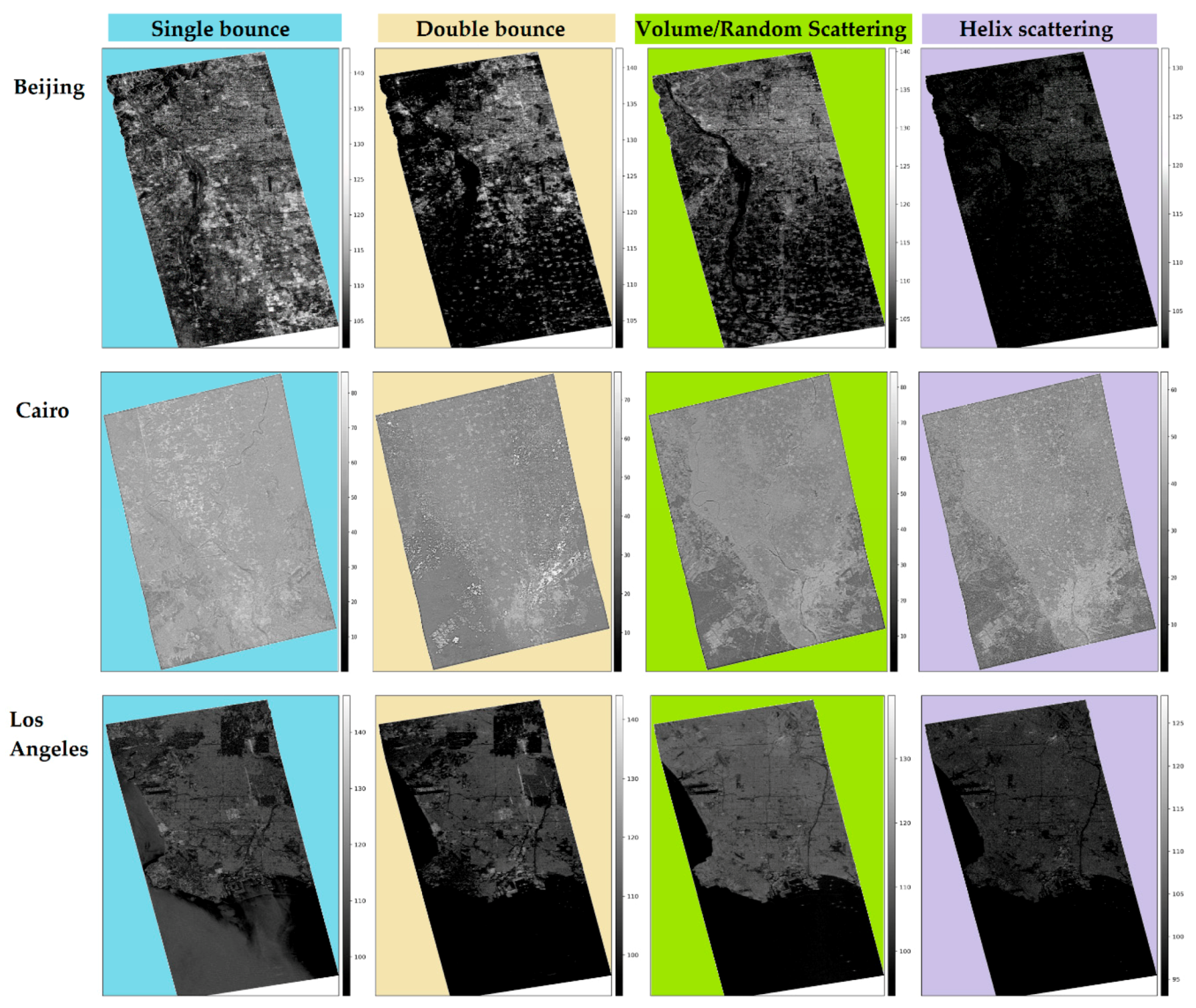
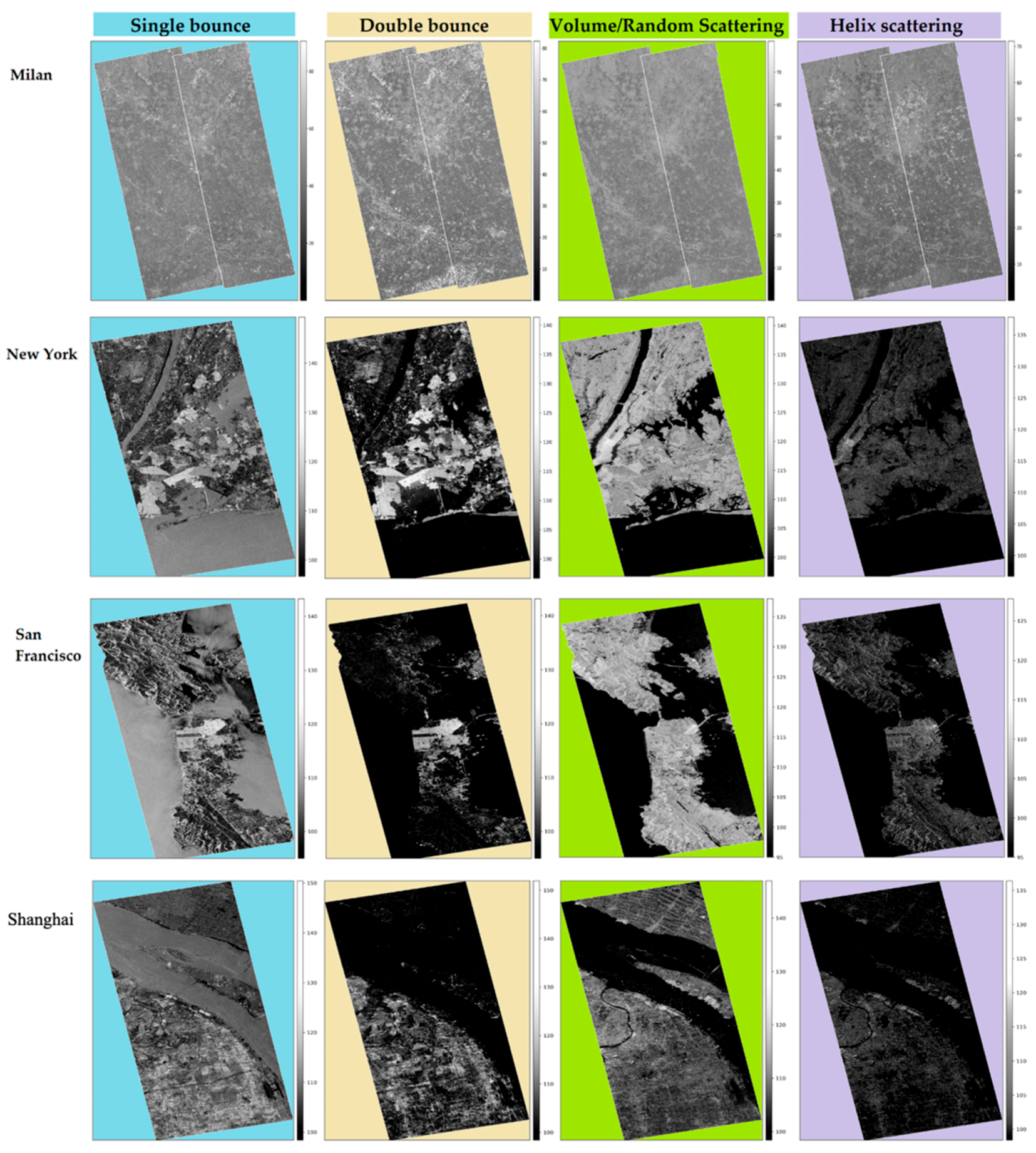
| City | Single Bounce [%] | Double Bounce [%] | Volume/Random Scattering [%] | Helix Scattering [%] |
|---|---|---|---|---|
| Beijing | 54.42 | 21.78 | 23.77 | 0.03 |
| Shanghai | 52.29 | 18.11 | 29.58 | 0.02 |
| Milan | 48.31 | 21.24 | 30.42 | 0.03 |
| New York | 22.62 | 20.11 | 57.24 | 0.03 |
| San Francisco | 31.35 | 10.27 | 58.37 | 0.01 |
| Los Angeles | 34.73 | 12.42 | 52.83 | 0.02 |
| Greater Cairo | 98.86 | 0.15 | 0.99 | 0.00 |
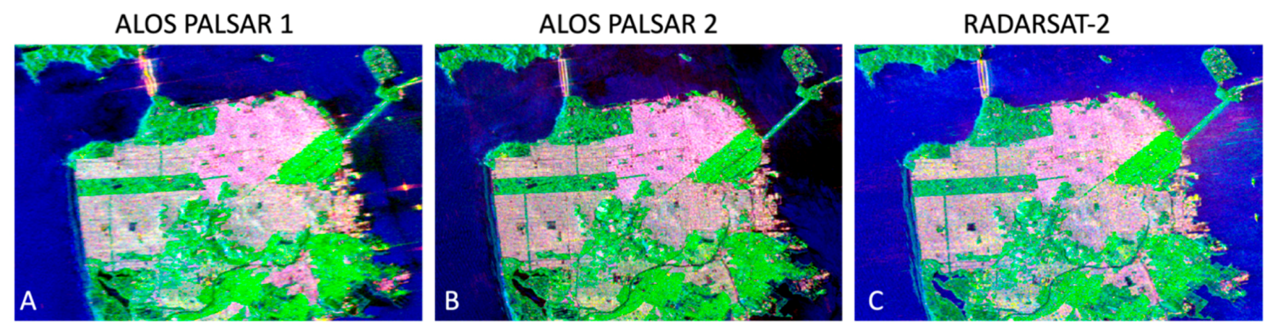
| Satellite | Acquisition Date | Frequency Band (GHz) | Spatial Resolution [m] | Incident Angle [degrees] |
|---|---|---|---|---|
| ALOS PALSAR 1 | 11/11/2009 | L (1.270) | 40 × 40 | 23.87 |
| ALOS PALSAR 2 | 24/03/2015 | L (1.236) | 6 × 6 | 33.87 |
| RADARSAT-2 | 09/04/2008 | C (5.404) | 8 × 8 | 28.9 |
| Scattering Mechanism Sensor | Single Bounce [%] | Double Bounce [%] | Volume/Random [%] | Helix [%] |
|---|---|---|---|---|
| ALOS PALSAR-1 | 36.68 | 14.87 | 48.43 | 0.02 |
| RADARSAR-2 | 34.53 | 24.15 | 40.8 | 0.52 |
| ALOS PALSAR-2 | 23.31 | 30.92 | 45.68 | 0.09 |
© 2020 by the authors. Licensee MDPI, Basel, Switzerland. This article is an open access article distributed under the terms and conditions of the Creative Commons Attribution (CC BY) license (http://creativecommons.org/licenses/by/4.0/).
Share and Cite
Delgado Blasco, J.M.; Fitrzyk, M.; Patruno, J.; Ruiz-Armenteros, A.M.; Marconcini, M. Effects on the Double Bounce Detection in Urban Areas Based on SAR Polarimetric Characteristics. Remote Sens. 2020, 12, 1187. https://doi.org/10.3390/rs12071187
Delgado Blasco JM, Fitrzyk M, Patruno J, Ruiz-Armenteros AM, Marconcini M. Effects on the Double Bounce Detection in Urban Areas Based on SAR Polarimetric Characteristics. Remote Sensing. 2020; 12(7):1187. https://doi.org/10.3390/rs12071187
Chicago/Turabian StyleDelgado Blasco, José Manuel, Magdalena Fitrzyk, Jolanda Patruno, Antonio Miguel Ruiz-Armenteros, and Mattia Marconcini. 2020. "Effects on the Double Bounce Detection in Urban Areas Based on SAR Polarimetric Characteristics" Remote Sensing 12, no. 7: 1187. https://doi.org/10.3390/rs12071187
APA StyleDelgado Blasco, J. M., Fitrzyk, M., Patruno, J., Ruiz-Armenteros, A. M., & Marconcini, M. (2020). Effects on the Double Bounce Detection in Urban Areas Based on SAR Polarimetric Characteristics. Remote Sensing, 12(7), 1187. https://doi.org/10.3390/rs12071187