Co-Seismic Magnetic Field Perturbations Detected by Swarm Three-Satellite Constellation

Abstract

The first 5.3 years of magnetic data from three Swarm satellites have been systematically analyzed, and possible co-seismic magnetic disturbances in the ionosphere were investigated just a few minutes after the occurrence of large earthquakes. We preferred to limit the investigation to a subset of earthquakes selected in function of depth and magnitude. After a systematic inspection of the available data around (in time and space) the seismic events, we found 12 Swarm satellite tracks with co-seismic disturbances possibly produced by ten earthquakes from Mw5.6 to Mw6.9. The distance of the satellite to the earthquake epicenter corresponds to the measured distance-time arrival of the disturbance from the surface to the ionosphere, confirming that the identified disturbances are most likely produced by the seismic events. Secondly, we found a good agreement with a model that combined a propagation of the disturbance to the F2 ionospheric layer with an acoustic gravity wave at a velocity of about (2.2 ± 0.3) km/s and a second faster phenomenon that transmits the disturbance from F2 layer to the Swarm satellite with a velocity of about (16 ± 3) km/s as an electromagnetic scattering propagation.

1. Introduction

This paper aimed to search for perturbations of the geomagnetic field in the ionosphere possibly produced by the occurrence of an earthquake in the lithosphere. The possibility that the ionosphere could be perturbed just a few minutes after the occurrence of a medium (Mw6+) and large (Mw7+) earthquakes is well known. For example, Yeh and Liu, 1974 [1] presented a model for the generation, propagation and response of the ionosphere to acoustic gravity waves. They also provided experimental data by supporting their model. Yamamoto, 1982 [2] theorized a model to describe the acoustic gravity waves induced by submarine earthquakes. Submarine earthquakes deserve special attention due to their potential to generate tsunamis. Lognonne et al., 2006 [3] observed the impact of the acoustic waves by the Global Positioning System (GPS) network 660–670 s (~11 min) after the arrival time of Rayleigh waves at the ground for the Mw7.9 November 3rd, 2002, Alaska earthquake. Hao et al., 2012 [4] reported not only ionospheric Doppler caused by the Mw9.0 Tohoku 2011 earthquake, but even geomagnetic disturbances from three different ground observatories. They carefully checked that the disturbances recorded on the ground were not caused by the ground shake due to the earthquake but as a magnetic effect. Jin et al., 2015 [5] presented a general review about the acoustic gravity waves produced by earthquakes and gravity waves generated by tsunamis, in particular focusing on the alteration of plasma density and velocity in ionosphere retrievable by the Global Navigation Satellite System (GNSS) global network sensors. Furthermore, they presented also a detailed analysis of the Mw7.8 Wenchuan 2008 and Mw9.0 Tohoku 2011 earthquakes.

Many authors [5,6,7,8,9] analyzed the Total Electron Content (TEC) variations from ground GNSS receivers and Global Ionospheric Map (GIM) and detected the impact of the acoustic gravity wave in the ionosphere associated with the occurrence of earthquakes. The analysis of TEC data has also shown to be a useful tool to detect the main earthquake parameters (epicentre and magnitude) using fast analysis techniques [10]. Rapoport et al., 2004 [11] proposed the acoustic gravity waves as a possible mechanism to explain disturbances prior to the occurrence of the earthquakes. They conducted three-dimensional (3D) simulations of the atmosphere and the ionosphere and found perturbations before some earthquakes. They also provided a possible explanation for the reason why the Outgoing Long-wave Radiation (OLR) anomalies generally are not found directly above the epicentre. As the authors suggested, this is only one of the various mechanisms for a possible pre-seismic alteration of the ionosphere. Other mechanisms are the possible electromagnetic coupling (e.g., [12,13]) or a more complex chain of physical, chemical and electromagnetic processes such as the one described by [14].

The aim of this paper is to study the potentiality of using magnetic data from space to identify co-seismic magnetic disturbances. In particular, the analysis will be focused in this investigation on the direction and value of the geomagnetic field as measured by satellites, with particular attention in the frequency band between 0.25 Hz and 0.50 Hz. The measurement of the geomagnetic field from space implies that the satellite is not necessarily close to the epicentral zone during and after the occurrence of the seismic event. Swarm satellites constellation has the advantage to be successful in orbit for more than five years and that as a constellation, it increases the probability of detection. Although the constellation is composed by three identical satellites, the probability of detection of the possible co-seismic signal is increased by a factor of about two as two of three satellites (Alpha and Charlie) fly close each other.

In Section 2, the earthquake catalogue, Swarm magnetic dataset and data analysis methods are presented. The results of the automatic analysis of Swarm magnetic data are reported in Section 3, and a possible propagation model is discussed in Section 4. Some conclusions are finally given in Section 5.

2. Datasets and Methods of Analysis

In this section, the used datasets and methodology are presented. In particular, in Section 2.1, we present the earthquake catalogue and the criteria to select the seismic events; Section 2.2 presents the magnetic satellite data of the European Space Agency (ESA) Swarm mission. Finally, Section 2.3 details the methods of analysis.

2.1. Earthquake Catalogue

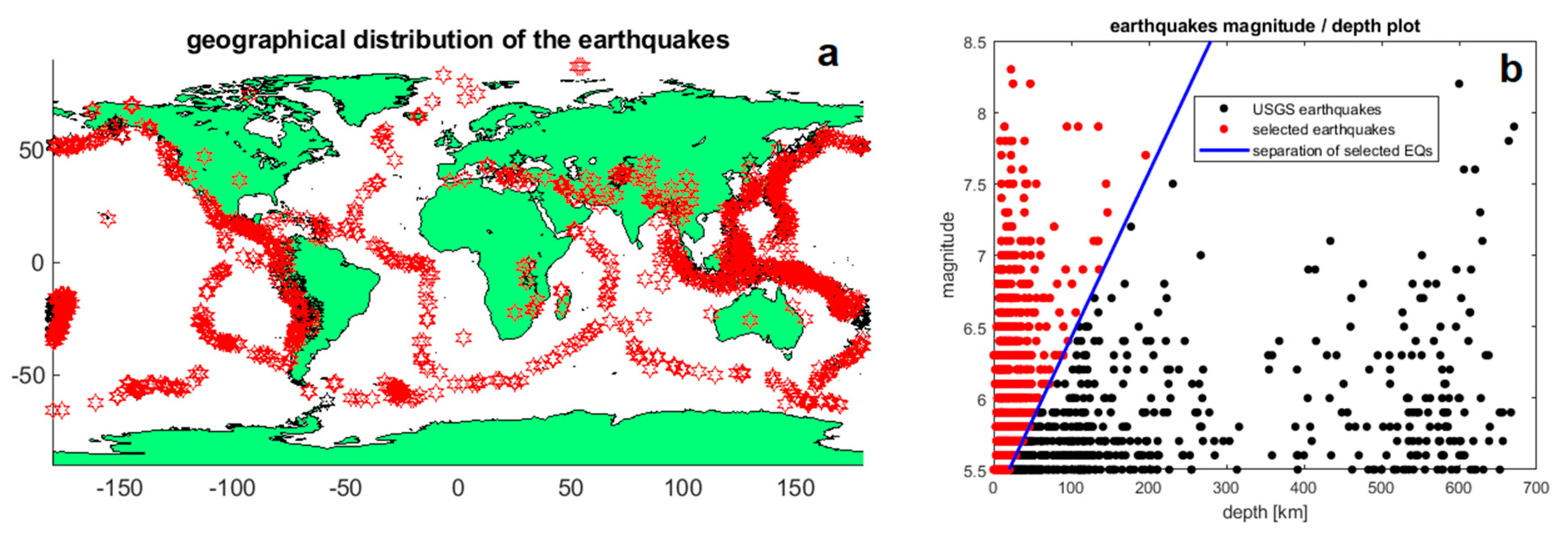
The seismic events were selected from the United States Geological Survey (USGS) catalogue. From the catalogue, all recorded events from 25 November 2013 to 12 April 2019 with a magnitude equal to or greater than 5.5 were downloaded and represented with a black star or dot in Figure 1 according to their geographical distribution (Figure 1a) and the magnitude/depth distribution (Figure 1b). Although some authors also included deep earthquakes in ionospheric disturbance investigations [15,16], we prefer to exclude them, as we consider the possibility that deep earthquakes could affect the ionosphere to be lower. To achieve this selection, all Mw5.5+ events up to 20 km depth were selected and for more in-depth events, a selection based on a higher magnitude and depth was applied. In particular, a linear interpolation was applied from Mw5.5 at 20 km and Mw7.0 at 150 km depth. This choice is a compromise to exclude the deeper earthquakes but not the strongest and deepest events that could produce a disturbance in the ionosphere because of their significant released energy. The number of the selected events was 1830 out of 2437 downloaded earthquakes, represented by a red star/dot in Figure 1. In particular, in Figure 1b it is possible to note the exclusion of the deepest events. The selected earthquakes are a sub-set in which it is more reliable to search for effects induced in the ionosphere, but future works can also investigate other events or subsets.

2.2. Swarm Satellite Magnetic Data

In this paper, the data from the ESA Swarm mission have been investigated. The main goal of the mission was to measure and monitor the Earth’s magnetic field with global coverage and better understand the electromagnetic phenomena on our planet [17]. Swarm is a three-identical satellite constellation successfully launched on 22 November 2013. The mission is still in orbit, and the present objective is to extend the mission for an entire solar cycle of 11 years. Most of the instruments continue to work in nominal conditions. Currently, more than five years of data are available.

The three satellites follow quasi-polar orbits: two of them (called Alpha and Charlie) fly close to each other at a lower orbit (around 450 km) and the other one, called Bravo, currently has a separation of about 90° longitude, and it is placed at a higher orbit, around 510 km. In the first months of the mission, all the satellites orbited close to each other.

Each satellite is equipped with the following payloads: Vector Field Magnetometer (VFM), Absolute Scalar Magnetometer (ASM), electric field instrument (EFI), accelerometers, GNSS receivers and laser retroreflectors. The VFM and ASM measure the orientation and intensity of the magnetic field. These sensors are placed on a 4-m length boom to avoid possible interferences with the satellite platform. The VFM sensor, placed half-way along the boom, is a fluxgate magnetometer with three-axis compact spherical coil with a three-axis compact detector coil inside. The magnetic field intensity calibration of the VFM is based on the data acquired by the ASM instrument placed at the end of the boom. For the Charlie satellite, the calibration is set on the data of Alpha ASM, as its ASM has not functioned since November 2013. The orientation of the VFM was precisely monitored with three star-tracker cameras placed on the same optical bank of the magnetometer.

The Swarm mission has already provided vast results; among them, a map of the lithospheric magnetic field with a resolution up to 250 km [18] and the oceanic tidal effect on geomagnetic field and electromagnetic induction generated by oceanic circulation (e.g., [19,20,21]). Furthermore, some of the authors of this paper found a series of anomalies in Swarm magnetic field and electron density data that could be related to the preparation phases of some earthquakes around the world (e.g., Mw7.8 Nepal 2015 [22], Mw8.2 Mexico 2017 [23], 2018, Mw6.5 Italy 2016 [24], Mw7.3 Iran 2017 [25], Mw7.5 Indonesia 2018 [26]). A recent paper by De Santis et al., 2019 [27] provided for the first time a worldwide statistical correlation of Swarm electron density and magnetic anomalies with earthquake occurrences, finding some distinct concentrations of anomalies that preceded the earthquakes from some days to several months; additionally, a linear dependency was established between the logarithm of the anticipation time of the anomaly and the earthquake magnitude, confirming for satellite data the empirical Rikitake law [28], which was already introduced for ground precursors.

The Swarm magnetic data have been downloaded from the free accessible FTP repository (swarm-diss.eo.esa.int) in Level 1B as CDF files with the filename SW_OPER_MAGx_LR_1B_[…], where x stands for A, B or C satellite and the filename is completed with the starting and ending timestamp of the file and the data version (408 for most of this work and 505 for the most recent data). MAG is the label that identifies the magnetic product and LR stands for Low Resolution (1 Hz) that is a product re-sampled from the original one (HR, i.e., High Resolution: 50 Hz) at the GPS seconds.

2.3. Methods to Analyze the Magnetic Satellite Data

A series of MATLAB^® routines have been developed to analyze the Swarm Magnetic data. The first script reads the earthquake catalogue and selects the events in agreement with the magnitude–depth requirements described in Section 2.1 (all earthquakes with Mw ≥ 5.5 and depth according to a linearly varying threshold from 20 km depth for Mw = 5.5 and Mw = 7.0 at 150 km depth). For each event, the algorithm selects the magnetic satellite data on the same date. The polar regions above a 70° geographical latitude are cut, as they are not suitable for this study due to the typical perturbation of the auroral activity. The goal of this work was to analyze the anomalous magnetic activity associated with earthquakes; thus, other magnetic perturbations, such as the geomagnetic storms, must first be rejected. After that, the script calculates the spatial distance of each sample from the epicentre and the time difference between the acquisition time and the earthquake origin time. If there are some samples close in space-time to the seismic event (distance ≤ 150 km and time difference from 10 min before until 20 min after the earthquake), the script selects and runs an automatic analysis of the close track.

Two types of automatic analyses have been performed: the first one is called Method 1, and it is the same proposed in previous works on Swarm data related to earthquakes (e.g., [22,24]. This technique consists of computing the first derivative of the data along the track approximated as the first difference divided for the time interval between two consecutive samples. After this step, a cubic spline is removed and the residuals of X, Y, Z (geomagnetic components) and F (intensity) are plotted with a fixed maximum range of ± 1 nT/s.

The second method (so-called Method 2) has been developed to avoid a possible over-fitting problem of the first method, i.e., that the spline could remove the eventual perturbation induced by the supposed gravity wave. It consists of the subtraction of the International Geomagnetic Reference Field (IGRF-12) model [29] from the original data and the plotting of the residuals in X, Y, Z and F. The IGRF-12 is a global Earth’s magnetic field model, which is expected to be sufficient to highlight the studied disturbances. A five-degree polynomial has been further applied to remove the residual trend of each track.

The output figures of both methods are presented in the Supplementary Materials. Each figure presents a map of the geographical region crossed by the satellite, the projection of the satellite track on the ground (brown for normal conditions and red for some abnormal conditions on the satellite) and the earthquake epicenter (green star). The title of the figure provides the satellites, the time in UTC and Local Time and the geomagnetic indices Dst and ap during the acquisition time. The residuals of X, Y, Z and F are reported together with the Fast Fourier Transform analysis of the signal that helps to select the best cut-off frequency for the following signal processing (for the second method, the mean of the signal is subtracted before calculating the FFT). The figures are grouped in tables that refer to each seismic event.

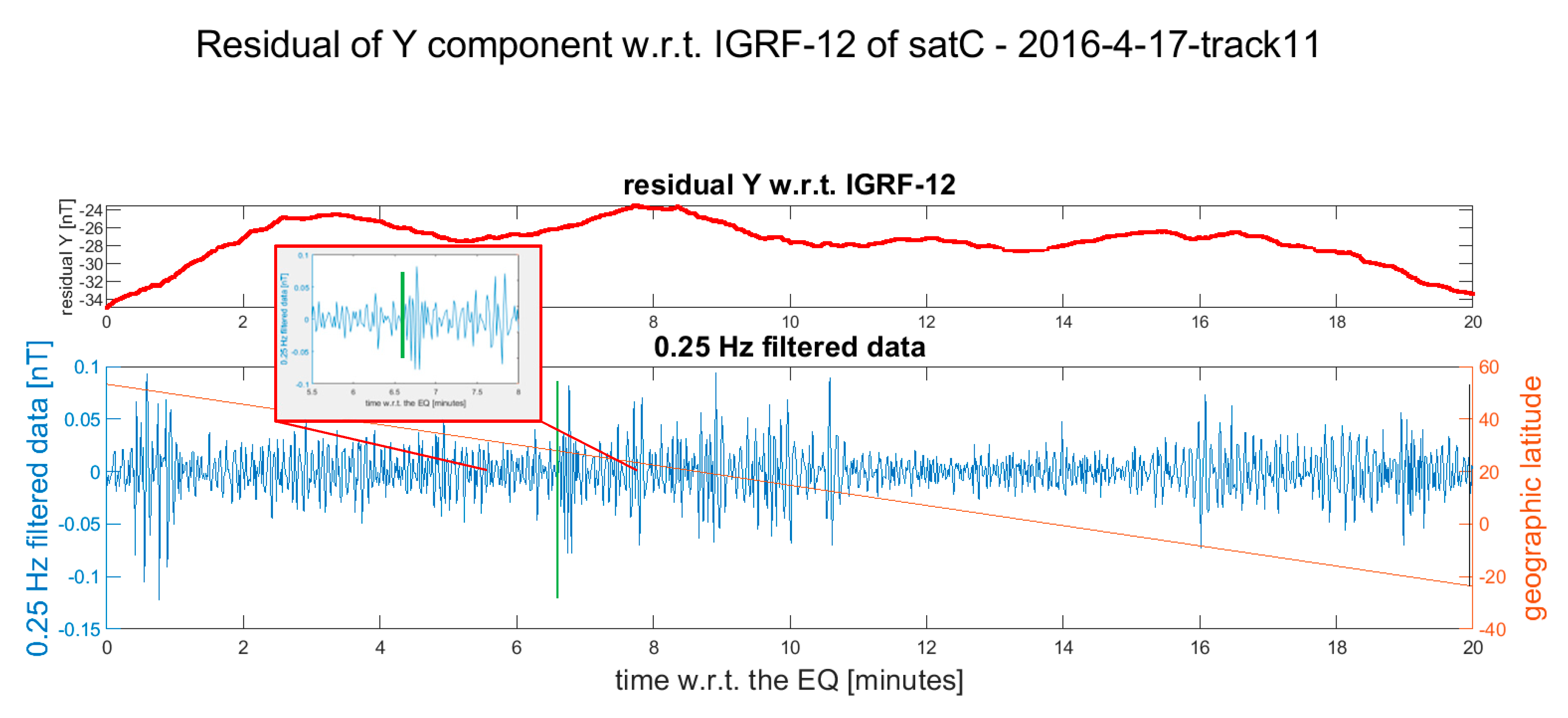
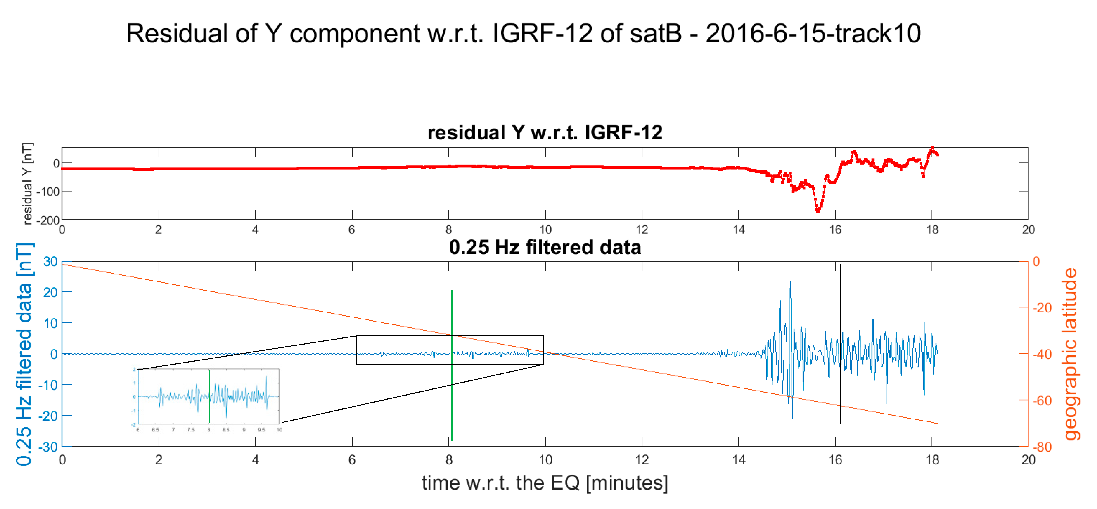
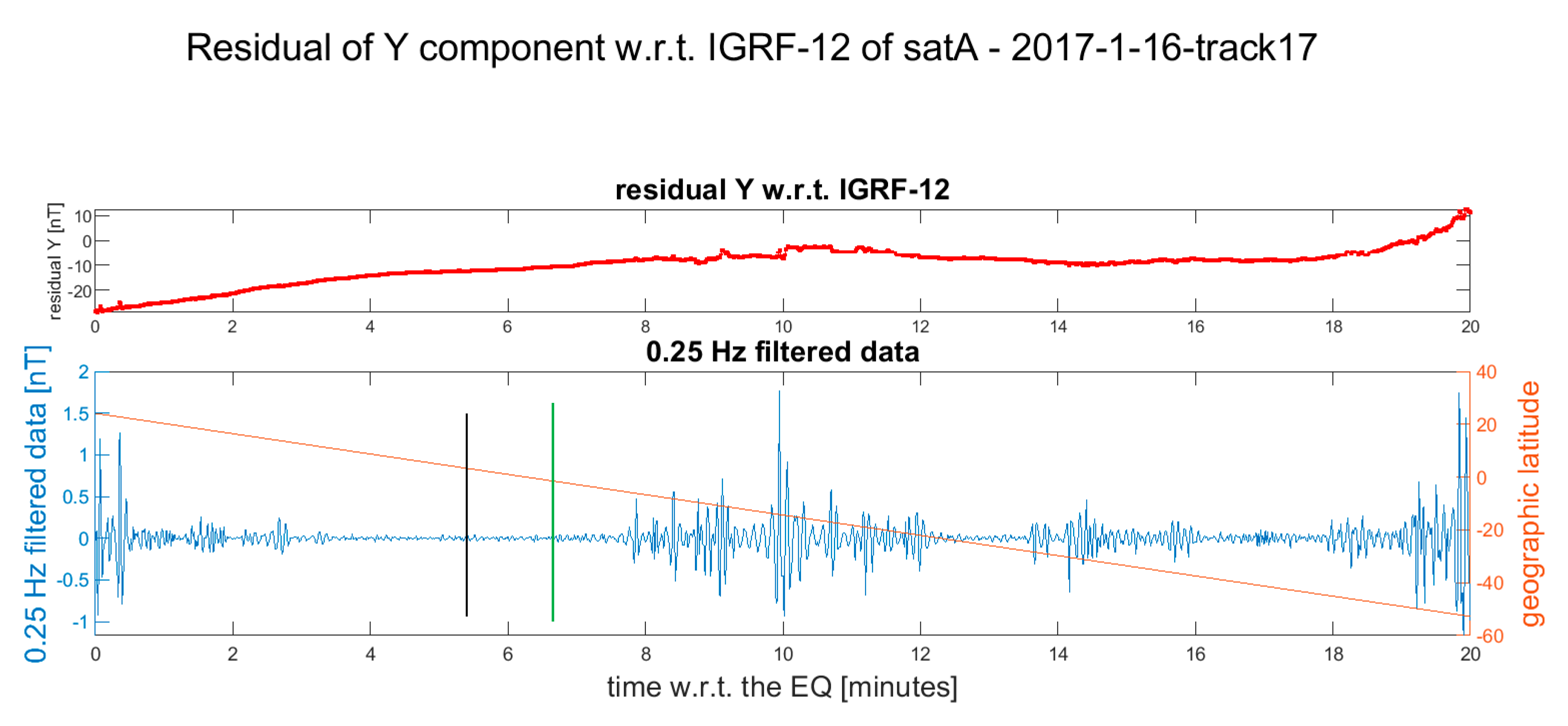
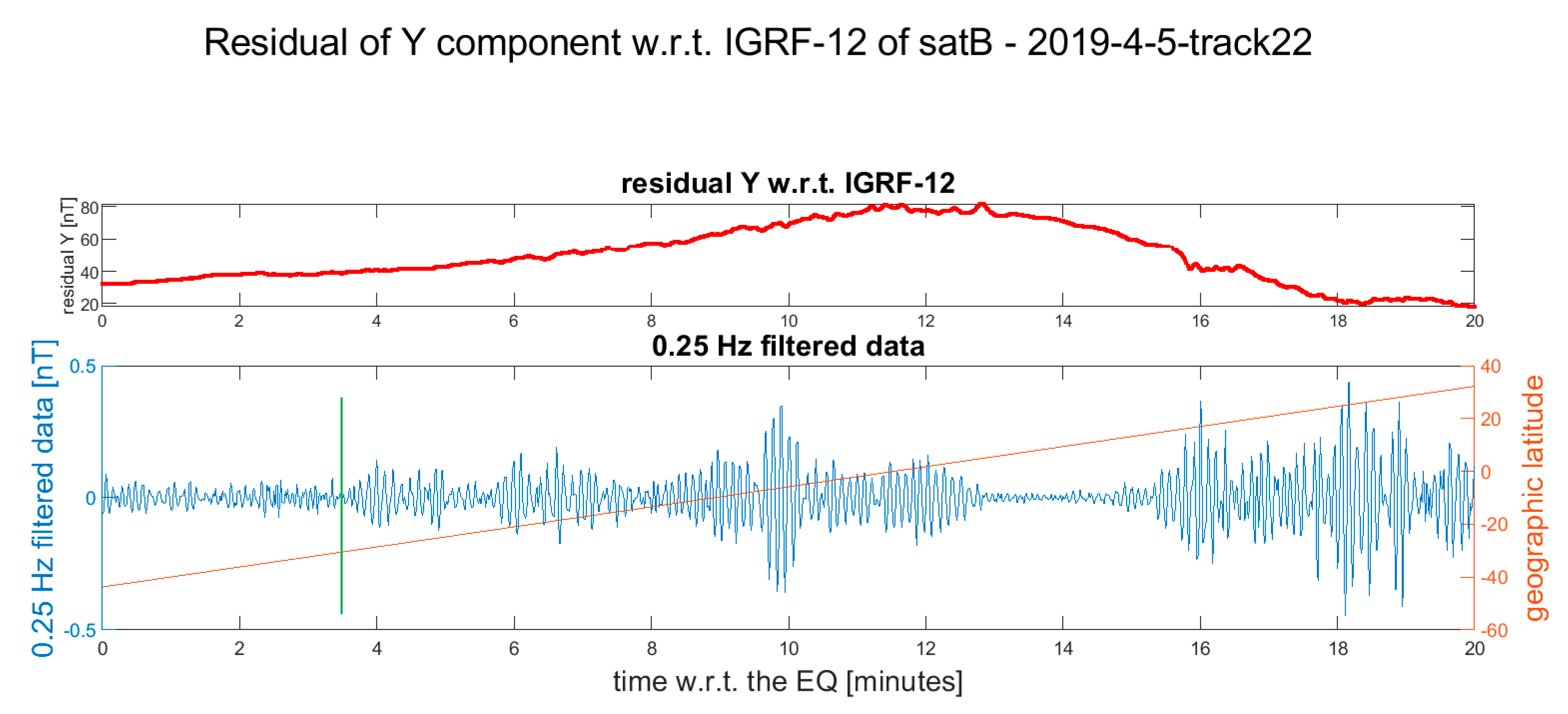
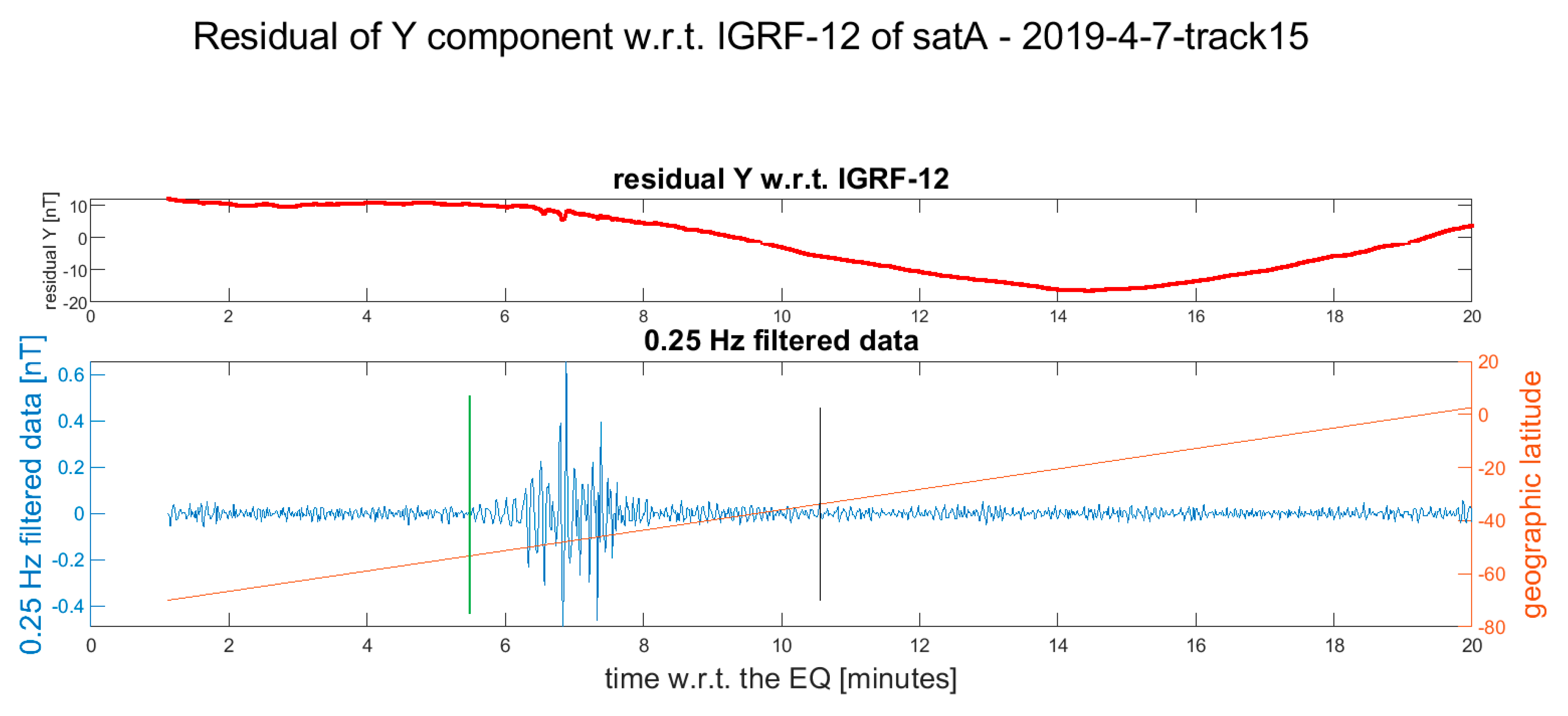
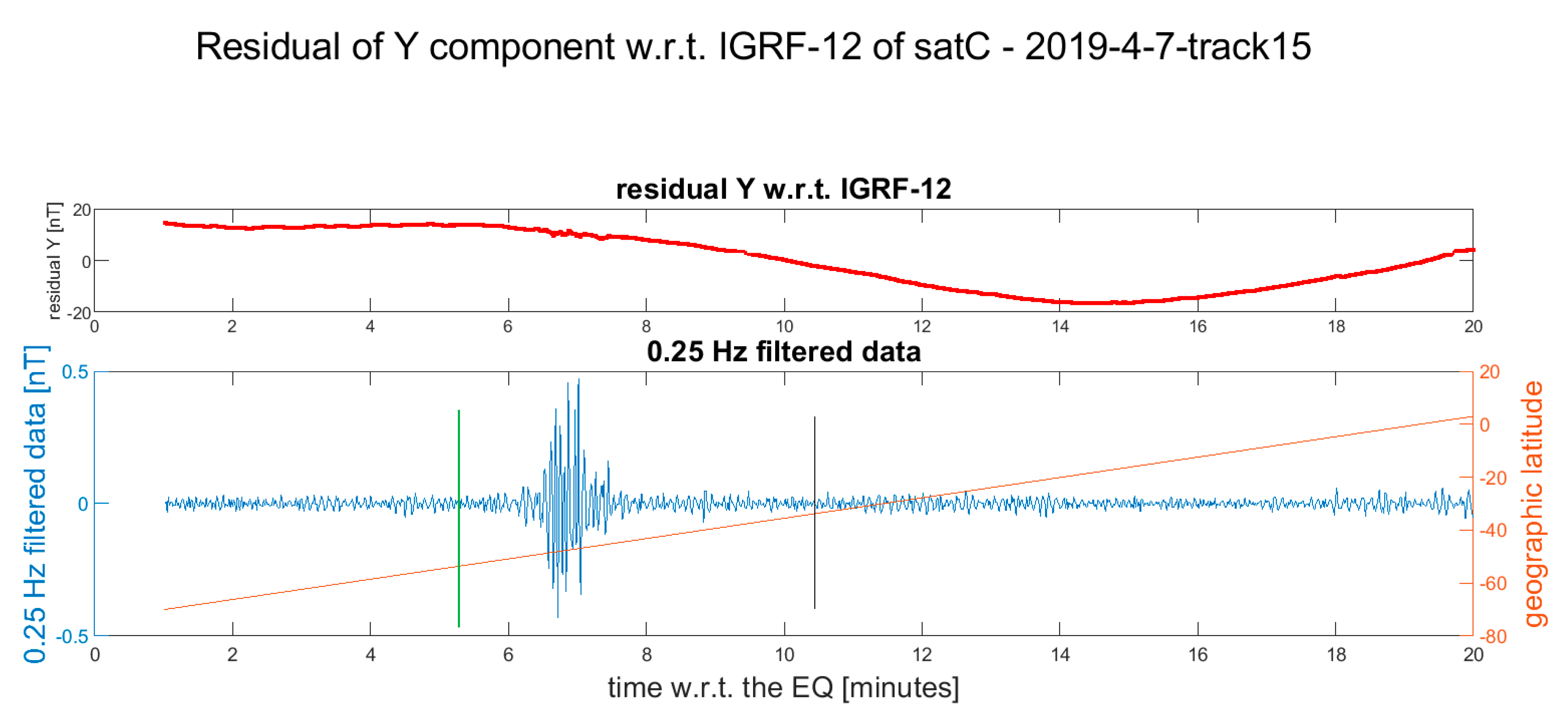
All the satellite data of the selected track are stored in a text file for further analysis. The produced material is visually investigated and the tracks that present some possible features linkable to the seismic events are then re-analyzed and plotted again. For this final analysis (presented in Figures 3–14), only the Y component is considered: after the subtraction of IGRF-12 model, a high pass filter at 0.25 Hz was applied and both quantities were then plotted. The frequency cut-off was chosen after multiple tests as the best value to extract the anomalous signal possibly related to the seismic event. Taking into account that the sampling rate of the data was 1 Hz, the available band was 0.25 Hz–0.50 Hz (following Nyquist theorem).

3. Results of the Analysis

From the launch of the mission on November 22^nd, 2013 until April 2019, the Swarm satellite data have been analyzed to search when one or more satellites passed above the epicentral area during an earthquake occurrence. To be conservative, a simultaneous passage was defined by a circular area of 150 km around the epicentre and a time window that spanned 10 min before the event until 20 min after. With such criteria, 37 satellite passages (tracks) were selected. For each case, method 1 and 2 were applied, searching for possible “interesting” features in the residual of at least one method. We finally noticed that even if the algorithm selected the space-time tracks closer to the epicenter, in some cases, the satellites passed too early or too late above the epicentral area, losing the chance to detect a co-seismic signal. After visually inspecting the residual plots, 12 tracks were considered the most likely candidate containing a co-seismic effect. 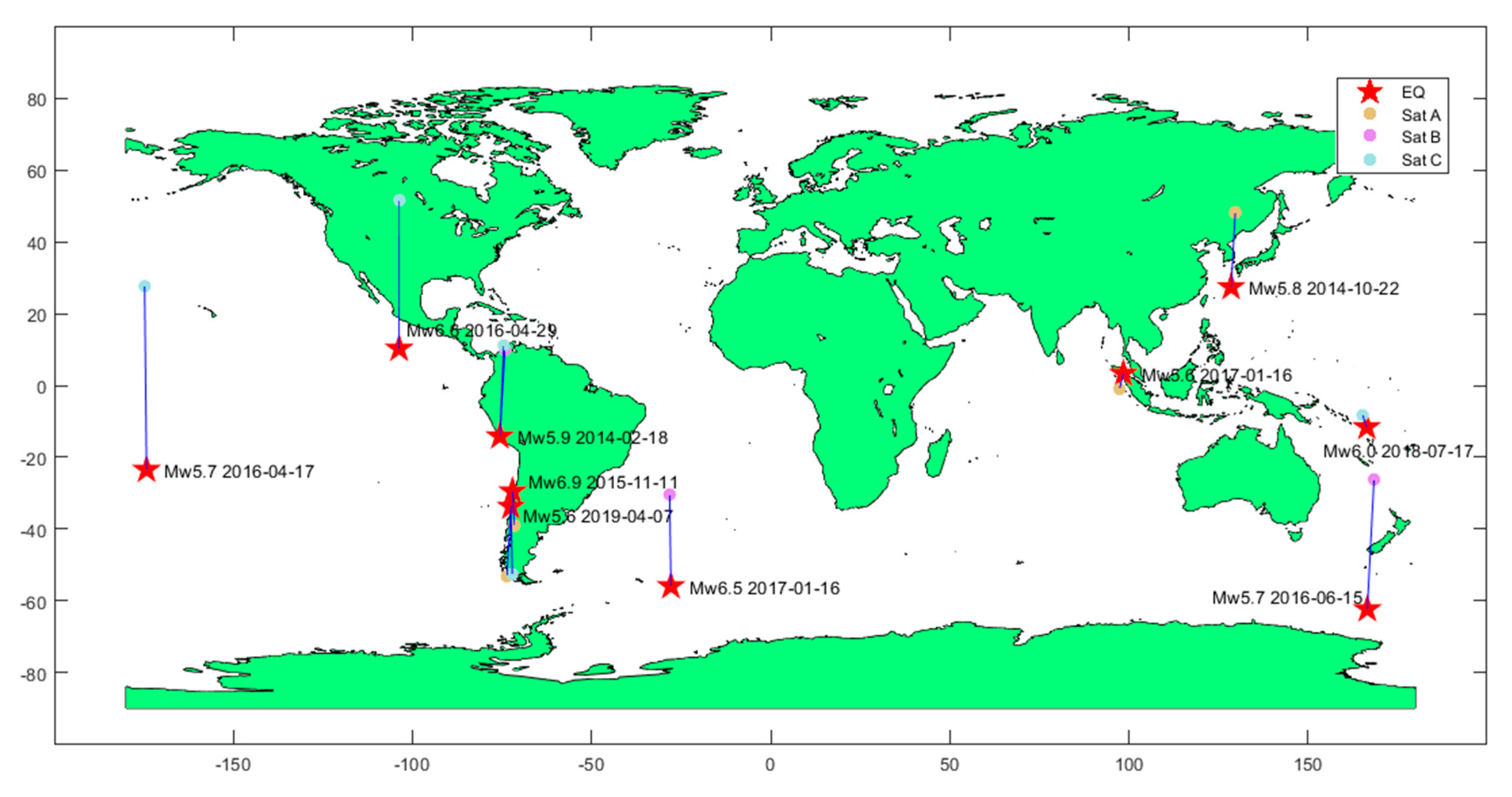Figure 2 reports the distribution map of the earthquakes and the ionospheric disturbances possibly associated with the seismic events.

Table 1. List of the earthquakes that created a potential magnetic disturbance in the ionosphere as detected from the Swarm satellite. The orbital characteristics are reported (satellite, direction of the semi-orbit: D for downward orbit, U for upward orbit, altitude, latitude and longitude) in the moment of disturbance detection. The height of the F2 ionospheric layer (hmF2) and the surface air temperature are also provided.

Earthquake Characteristics						Satellite Characteristics					Air Temperature [K]	hmF2 [km]	Relative Characteristics
Year-Month-Day	Hour-Minute-Second	Lat	Long	Mag	Depth [km]	SAT	D/U	Altitude [km]	Lat Sat	Long Sat			Lorizontal Distance [km]	Total Distance [km]	Measured Time [min]
2014-02-18	23:35:58	−14.165	−75.6	5.9	57.0	B	D	500.2	10.003	−74.187	292	454	2687	2733.2	5.151
						C	D	499.5	11.164	−74.514	292	454	2814	2858.0	6.184
2014-10-22	00:15:17	27.416	128.553	5.8	43.0	A	U	462.6	48.228	129.711	292	254	2312	2357.8	4.617
2015-11-11	02:46:19	−29.51	−72.058	6.9	10.0	A	U	463.7	−39.037	−71.541	289	368	1059	1156.1	3.050
2016-04-17	07:31:00	−23.495	−174.247	5.7	10.0	C	D	449.5	27.676	−174.798	296	268	5680	5697.8	6.650
2016-04-29	01:33:38	10.275	−103.736	6.6	10.0	C	D	444.9	51.651	−103.638	305	321	4593	4614.5	8.050
2016-06-15	06:58:27	−62.366	166.58	5.7	10.0	B	D	518.7	−26.200	168.448	266	310	4017	4050.3	6.550
2017-01-16	12:42:10	3.317	98.47	5.6	6.0	A	D	451.1	−0.973	97.400	297	349	4907	4927.7	6.517
2018-07-17	07:02:53	−11.594	166.432	6.0	38.0	C	D	448.0	−8.287	165.250	301	271	3891	3916.7	8.683
2019-04-05	16:14:16	−55.932	−27.846	6.4	58.4	B	U	510.0	−30.412	−28.208	274	231	2833	2878.5	3.517
2019-04-07	10:52:41	−33.764	−72.521	5.6	10.0	A	U	470.0	−53.197	−73.643	290	288	2159	2209.6	5.517
						C	U	470.0	−52.592	−72.142	290	288	1884	2090.0	5.567

reports the list of the earthquakes that present a possible magnetic disturbance in the ionosphere with the Swarm satellite characteristics in the moment of disturbance detection. The measured time is that after the origin time of the earthquake in which the anomaly starts to be detected by the Swarm satellite. The table also reports the height in km of the ionospheric F2 electron density peak (hmF2) estimated by the IRI-2016 model [30] and the air temperature at 2 m retrieved from the European Centre for Medium-range Weather Forecast (ECMWF) ERA-Interim archive, which will be used for the discussion and interpretation of the results.

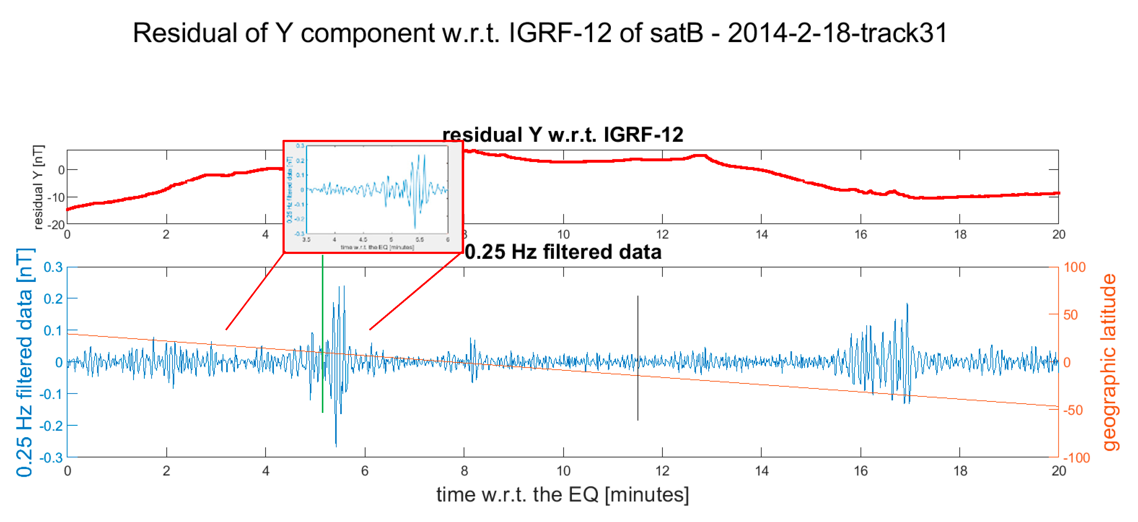
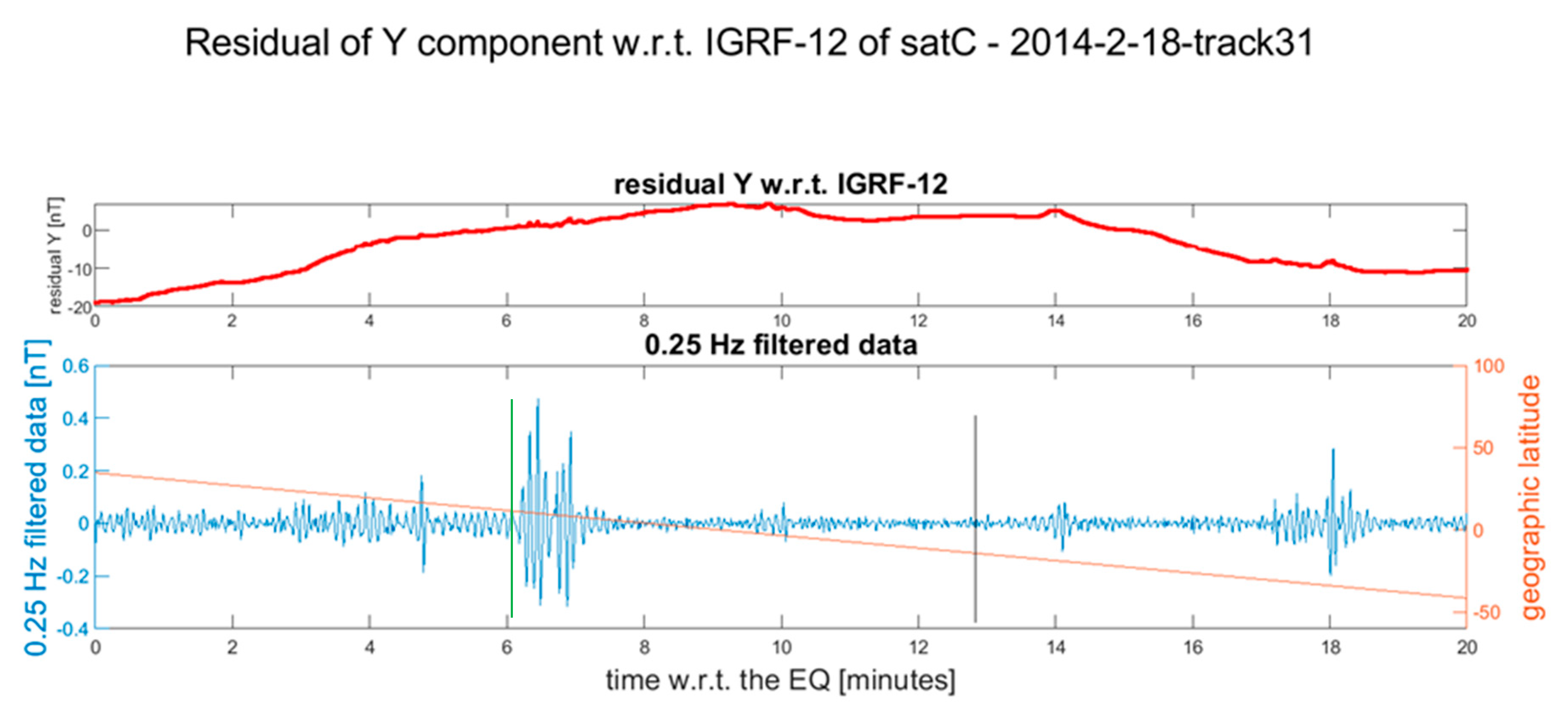
The Swarm magnetic data during the earthquake occurrence are represented following the same order of Table 1, i.e., a chronological one, from Figure 3, Figure 4, Figure 5, Figure 6, Figure 7, Figure 8, Figure 9, Figure 10, Figure 11, Figure 12 and Figure 13. Each figure is horizontally aligned with the origin time of the earthquake. In the upper part is shown in red the residual of the Y component of the magnetic field with respect to the IGRF-12 model. The Y component was selected as it is the most sensible for the internal perturbations ([22,31]). In the lower graph, a 0.25 Hz high-pass filter was applied, and the filtered data are shown in blue. Here, we did not subtract any polynomial, as the filter was sufficient to remove the residual trend. A black vertical line underlines the position where the satellite crosses the earthquake latitude if it is after the earthquake occurrence. An orange line represents the latitude of the satellite. Note that only the data inside −70° and +70° geographical latitude are shown. More details are provided in the Supplementary Materials, where Figures S1–S10 show the residuals of the other components as well as the total intensity of the magnetic field, as deduced using method 1 and method 2. Figure S11 also shows an example of a track without any evidence of possible co-seismic magnetic disturbance. The reasons for the lack of disturbance in the latter case could be several: the earthquake happened in the Atlantic ocean ridge and the ocean water depth at the epicentre is of several kilometres (about 3.4 km), thus possibly attenuating the mechanical effect (also considering the low magnitude of the event: Mw 5.5); another reason could be an intrinsic disturbance in the magnetic signal all over the track that could cover the detection of any small co-seismic effect. On the other hand, in the Figures S1–S10, the magnetic disturbance cannot be explainable merely by geomagnetic activity, which was low at the acquisition time; nevertheless, it could be induced by some other geophysical source (such as electric and magnetic fields produced by ocean currents—Grayver et al., 2016—or tectonic stress along the ocean drift).

The acoustic gravity waves induced by seismic activities are only a type of a great variety of phenomena that could affect the ionosphere. For this reason, several disturbances affect these figures. Therefore, to measure the time of the arrival of the possible disturbance induced by the seismic event, a particular change in the waveform, concentrating in the part of the track that started after some minutes of the seismic event, was selected. We excluded the first minute of each track, because an acoustic gravity wave requires about 3.5 min to reach Swarm altitude (~450km or more). The latitude of the satellite was also taken into account to understand if the disturbance could be due to the standard geomagnetic activity of the Earth’s polar regions. We admit that this interpretation is not totally objective and unique, although sufficiently reasonable. For a quick comparison and validation, we also present in the Appendix A an automatic approach that is totally objective and practically confirms our results.

For the earthquake that occurred on 2014-02-18, only the tracks of Bravo and Charlie (Figure 3 and Figure 4) are provided as Swarm Alpha was not in nominal conditions during the passage over the epicentral area. Most of the data present a discrepancy between ASM and VFM measurements (Flag_F = 16), and the attitude information was interpolated with the nearest points for lack of data from two or all three star-cameras. These conditions were probably due to the early stage of the mission that we analyzed.

An earthquake happened offshore Chile on 2015-11-11 at a depth of 10 km between the Nazca and South-American plates. In this case, a perturbation was visible just north of the epicentre and we cannot exclude that this could be an electromagnetic phenomenon coming directly from the fault. There was a certain symmetry of the signal with respect to the epicentre latitude. The ionospheric disturbance was possibly associated with the high magnitude earthquake (Mw 6.9) considered in this case (Figure 6).

4. Discussion and Interpretation

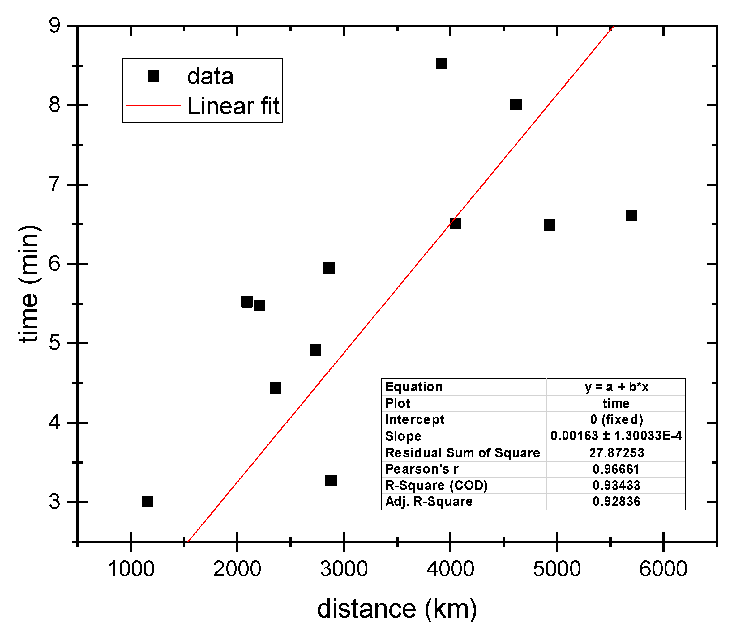
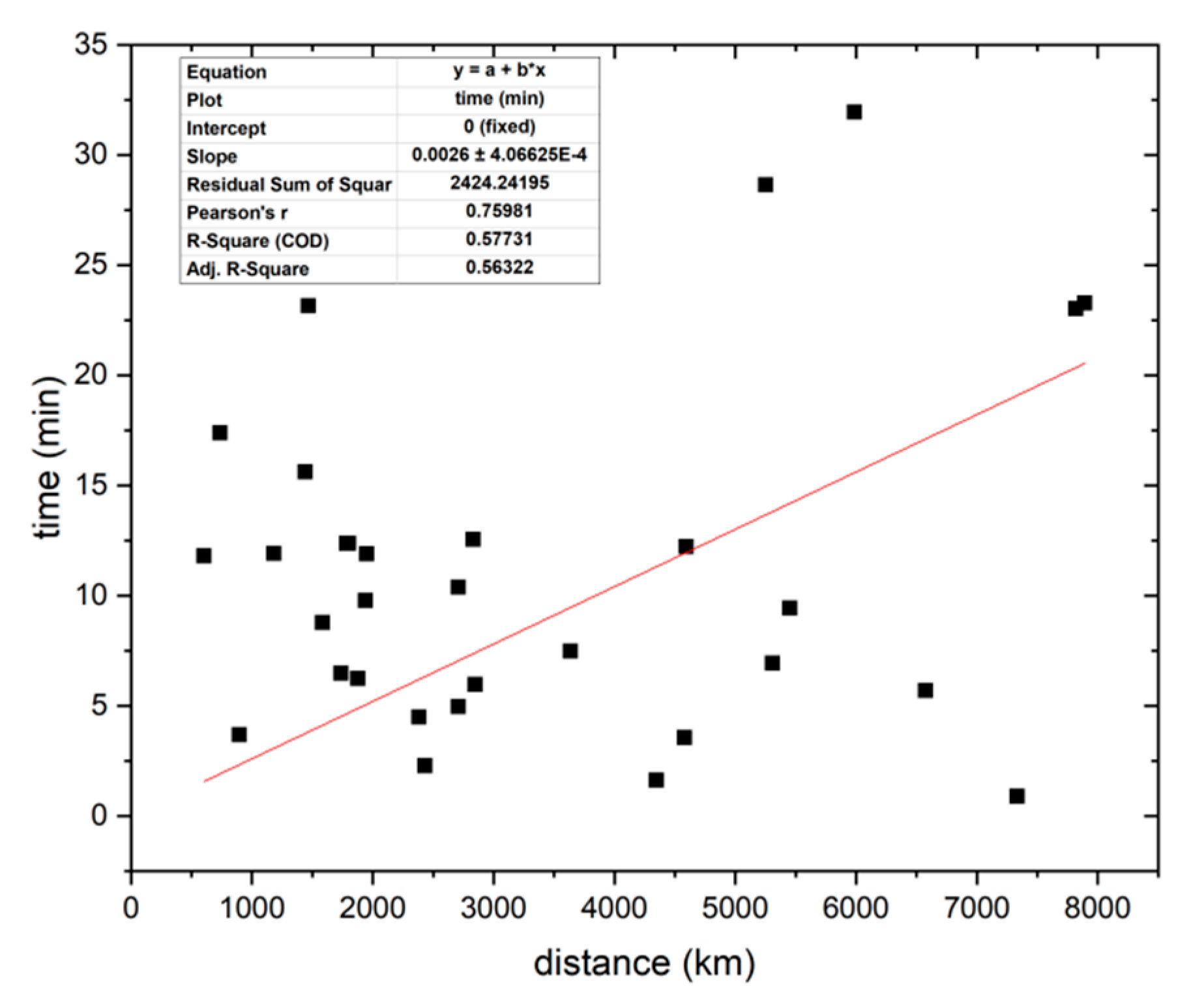
The 12 selected tracks associated to 10 seismic events have been analyzed to search for a possible linear regression between the time interval of the arrival of a supposed co-seismic gravity wave in the ionosphere and the distance between the epicentre and the Swarm satellite, as represented in Figure 14. The intercept has been fixed to the origin of the axis as the time to cover a null distance needs to be zero. The obtained slope is (0.00163 ± 0.00014) min/km that corresponds to a propagation velocity of (10.04 ± 0.85) km/s. The R² = 0.92 denotes a good agreement with this linear regression, confirming that the two quantities plotted in the graph seem to be linearly correlated. Although this correlation is pretty good, the propagation speed for this phenomenon seems to be higher than we might expect for this kind of waves. We propose that actually this could be caused by two different involved phenomena: one from the Earth’s surface that reaches the maximum electron density altitude (hmF2 or altitude of ionospheric layer F2), and another physical phenomenon that propagates from this altitude to the satellite position.

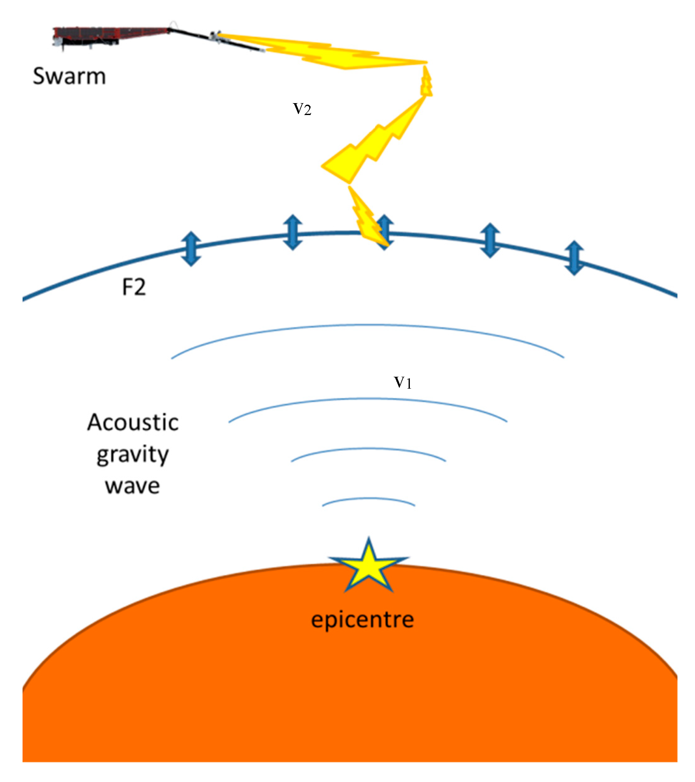
A sketch of the proposed propagation mechanism is shown in Figure 15. A simple model was implemented with a vertical propagation with velocity v₁ until hmF2 and a second velocity v₂ from the projection of the epicentre at hmF2 until the satellite position. The altitude of the F2 layer was determined by the IRI-2016 model and listed in Table 1. We supposed that the velocity v₁ and v₂ were equal for all the events, and thus, we determined which combination of v₁ and v₂ can reduce the difference with the measured times. “v₁” and “v₂” were selected in the range between 0.10 km/s and 50.00 km/s with a step of 0.01 km/s. We also take into account that the different air temperature T affects the mechanical velocity of propagation by a factor of $\sqrt{T}$ [32]. Thus, the surface (2 m height) temperature has been retrieved from the climatological archive ECMWF ERA-Interim for the 10 earthquakes, and the velocity v₁ was multiplied by $\sqrt{T/298K}$. The division by 298K assures to obtain the result referred to the standard temperature of 25 °C. The best combination that fits our data (i.e., the one with the minimum residuals) was v₁ = 2.20 km/s (at temperature of 25 °C) and v₂ = 16.07 km/s. From the dispersion of the measurements versus the model, we estimated an uncertainty on the velocities of about Δv₁ = 0.3 km/s and Δv₂ = 3 km/s. We note that the velocity v₁ is in agreement with the known velocities in the literature for acoustic gravity waves (e.g., [9]).

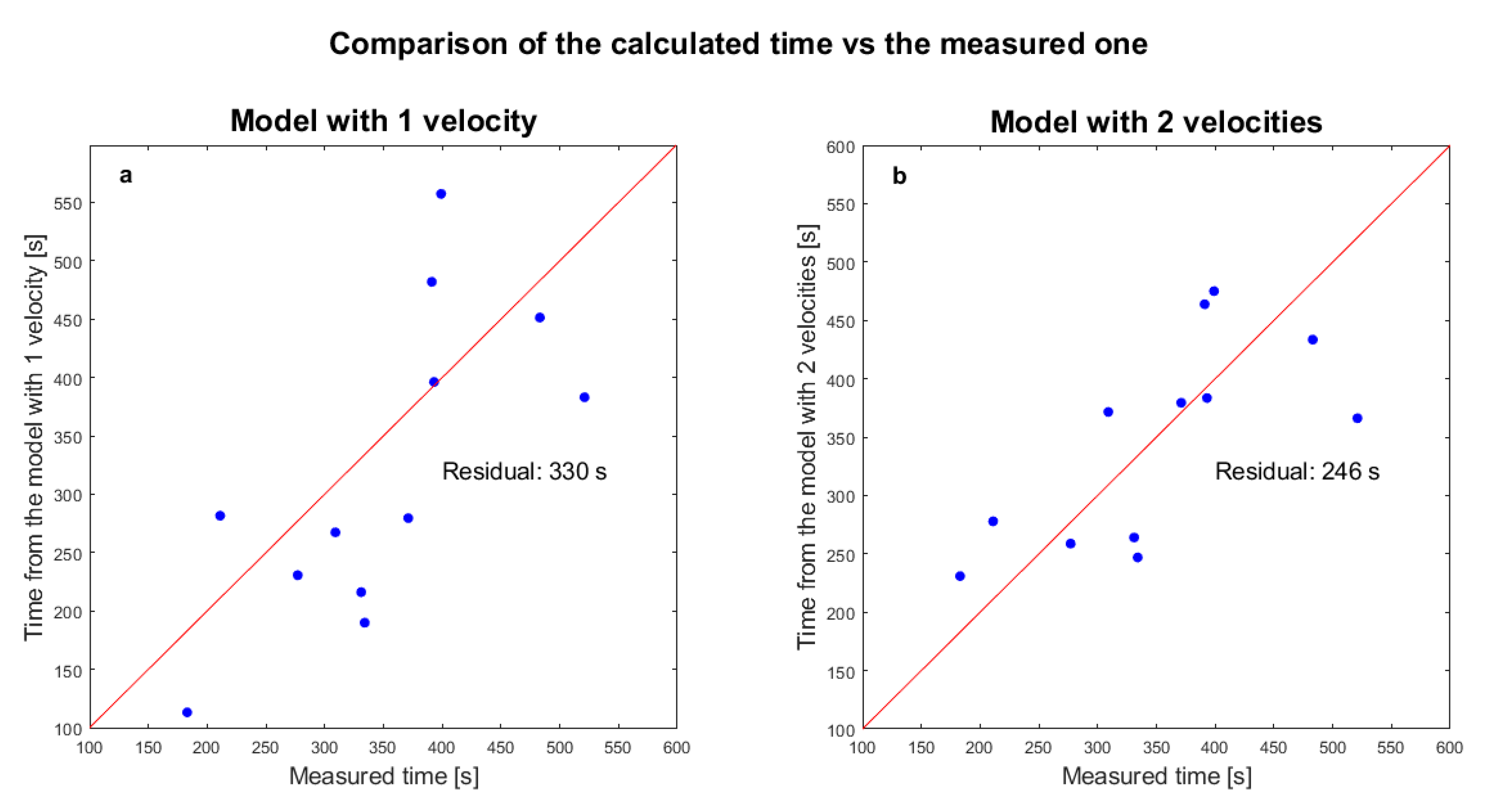
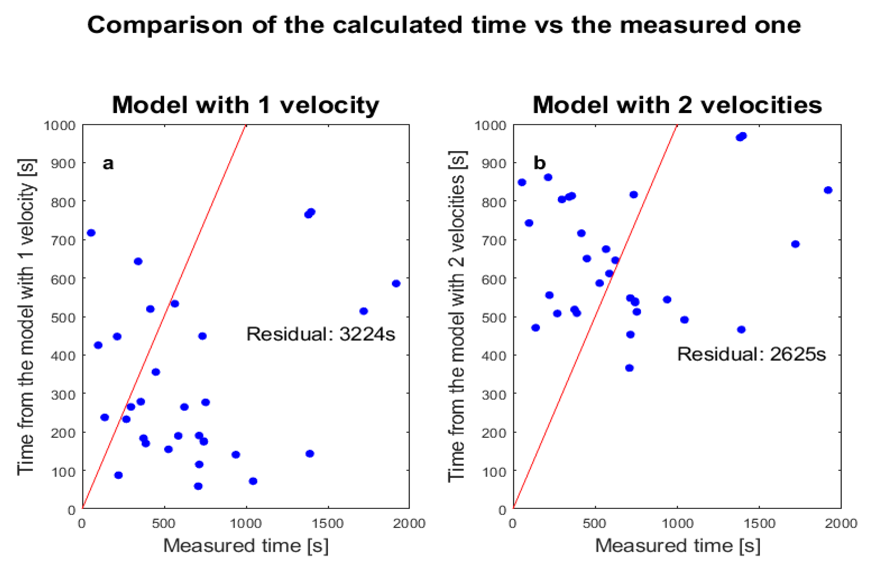
A comparison between the calculated and the measured times needed to propagate from epicentre to the satellite is represented in Figure 16. The red line represents the ideal case, i.e., when the model was identical to the measurements. The sum of the residual between the time estimated from the model and the measured one from satellite data was reported. The calculated values for the model with two velocities used the best-obtained velocity estimations. We note that in the second model (b), two cases were correctly described by the model as they are on the ideal trend, while the others were under- or overestimated. As also underlined by the lower value of the sum of the residuals, the model with two velocities estimates better the time of propagation of the disturbance from the epicenter to the satellite, with a lower dispersion of data in the plot and closer to the ideal case (red line). This statistical evidence deposes in favour of our assumption of a gravity wave that mechanically propagates until F2 layer making oscillating the high number of free electrons in this region and starting a scattering that propagates at least to the Swarm satellite altitudes (about 440–500 km above sea level). Considering also some literature [33,34], we tested the possibility that the second propagation follows the magnetic field lines strictly. We found that the results were worse than the simple straight propagation, thus, even if the perturbation could affect the magnetic field, the disturbance probably did not strictly follow the magnetic field lines.

To finally compare the two approaches describing the data (one-velocity or two-velocity model), we used the Akaike Information Criterion (AIC) developed by Akaike, 1973 [35]. In case of few parameters a “corrected” index AICc can be used. This criterion was used to choose the best model (the one that presents the minimum AIC, or AICc, later described) and select which variables were really fundamental to the system. The AIC is defined as:

$$AIC=2K-2 \log \left(L\right)$$

(1)

where K is the number of estimated parameters, i.e., the degree of freedom and L is the maximum of the likelihood function. For this paper, we used the following equation to estimate the $\log \left(L\right)$:

$$\log \left(L\right)=-\frac{1}{2}n{\sigma }^2=-\frac{1}{2}n{\left(\frac{RSS}{n}\right)}^2$$

(2)

where n is the number of samples and RSS is the Residual Sum of Squares. If the dataset on which the model is evaluated contains a small number of elements, as in our case, a correction factor must be introduced, estimating a second coefficient, called AICc:

$$AICc=AIC+\frac{2K\left(K+1\right)}{n-K-1}$$

(3)

To calculate the values of AIC and AICc for our two models, we followed the approach of Snipes and Taylor, 2014 [36], even if they applied this criterion to a vastly different case study.

Table 2. Results of the Akaike Information Criterion applied to the two used models.

	Number of Parameters K	Number of Samples	Residual Sum of Square RSS [s2]	AIC	AICc
Model 1 (one velocity)	2	12	1.09 × 105	99.0	100.3
Model 2 (two velocities)	3	12	6.07 × 104	94.9	97.9

reports the parameters and the AIC and AICc coefficients obtained for the two models. The number of parameters has been increased by one to consider an error coefficient in the model. Despite the height of the F2 layer (hmF2) and the temperature are two parameters used in the second model, they do not add any degree of freedom to the same model, since they are fixed.

The AICc (and even AIC) suggests that the model with two velocities better describes the magnetic disturbance identified in the 12-track dataset. From a physical point of view, this is promising, since the model with one velocity gives a speed that is not compatible with known phenomena of the interaction of lithosphere, atmosphere and ionosphere; otherwise, the first velocity of the second model is compatible with an acoustic gravity wave.

5. Conclusions

After a systematic analysis of the first 5.3 years of Swarm magnetic data around the Mw5.5+ earthquakes, we found that 12 Swarm satellite tracks recorded disturbances following earthquakes of magnitude Mw5.6 to 6.9. We underline that we limited our search for possible co-seismic effects to a subset of earthquakes selected in function of their depth and magnitude. Even if this subset could exclude some possibility to record some additional effect, we were driven by the necessity to exclude the deeper and lower magnitude events that are unfeasible to produce any seismic effect in the ionosphere. In addition, we do not expect particular difference with other selection criteria.

However, more energetic seismic events were recorded during this period (included three Mw8+ earthquakes: two in Chile and one in Mexico), but we did not find possible co-seismic ionospheric disturbances produced by these large events. This is due to the fact that the Swarm satellites did not fly just over the epicentral area at the time of the earthquake occurrence. This explains why we found geomagnetic ionospheric disturbances only for almost medium magnitude earthquakes.

The linear regression of the time versus the distance between the earthquake occurrence and the record of the disturbance by Swarm satellites seems to confirm that the seismic events possibly induce the disturbances.

To explain these disturbances, a model that combines two different propagation ways has been proposed with promising result. The model considers an acoustic gravity wave as the way to propagate the earthquake disturbance up to the F2 ionospheric layer, i.e., the layer with the maximum ionisation. The impact of the acoustic gravity waves on this layer could induce some electromagnetic scattering that propagates in the upper ionospheric layer, reaching the Swarm satellites. The propagation velocities, according to our data, are (2.2 ± 0.3) km/s with a 25 °C of surface air temperature for the acoustic gravity waves and (16 ± 3) km/s for the electromagnetic scattering propagation. We note that the approximation to the same velocity for all the seismic events is a limitation and, in particular, it does not take into account, e.g., the different local time: future improvements could introduce the importance of the local time together with some other parameters that would take into account the different chemical and physical conditions of the atmosphere and ionosphere where the phenomena propagate. This double-velocity model has better statistical reliability, providing a lower AIC than the one with only one velocity.

In order to validate the mostly subjective criteria chosen in this work to select the co-seismic anomalies, we developed an automatic algorithm that detects the co-seismic perturbations based on objective criteria (see Appendix A). The principal results of this paper were also confirmed by this automatic approach to detect the anomalies. Nevertheless, the automatic system was not yet able to achieve the quality with which a researcher can evaluate the signal of the satellite track to discriminate and choose the effects and causes of the detected disturbances. A future improvement of the automatic procedure can include the analysis of the signal frequency for not only searching a disturbance along the satellite track but also some particular frequencies without usually presenting in other parts of the track.

A larger constellation of Low Earth Orbit satellites equipped with magnetometers could improve the coverage, i.e., the capability to record and deeper understand this type of signal. The recent launch of the Chinese Seismo-electromagnetic satellite in 2018 could contribute to this endeavour greatly.

References

1. Yeh, K.C.; Liu, C.H. Acoustic-gravity waves in the upper atmosphere. Rev. Geophys. 1974, 12, 193–216. [Google Scholar] [CrossRef]
2. Yamamoto, T. Gravity waves and acoustic waves generated by submarine earthquakes. International J. Soil Dyn. Earthq. Eng. 1982, 1, 75–82. [Google Scholar] [CrossRef]
3. Lognonne, P.; Artru, J.; Garcia, R.; Crespon, F.; Ducic, V.; Jeansou, E.; Occhipinti, G.; Helbert, G.; Moreaux, G.; Godet, P.-E. Ground-based GPS imaging of ionospheric post-seismic signal. Planet. Space Sci. 2006, 54, 528–540. [Google Scholar] [CrossRef]
4. Jin, S.; Occhipinti, G.; Jin, R. GNSS ionospheric seismology: Recent observation evidences and characteristics. Earth-Sci. Rev. 2015, 147, 54–64. [Google Scholar] [CrossRef]
5. Laštovička, J.; Baše, J.; Hruška, F.; Chum, J.; Šindelářová, T.; Horálek, J.; Zedník, J.; Krasnov, V. Simultaneous infrasonic, seismic, magnetic and ionospheric observations in an earthquake epicentre. J. Atmos. Sol. Terr. Phys. 2010, 72, 1231–1240. [Google Scholar] [CrossRef]
6. Rolland, L.M.; Lognonné, P.; Munekane, H. Detection and modeling of Rayleigh wave induced patterns in the ionosphere. J. Geophys. Res. 2011, 116, A05320. [Google Scholar] [CrossRef] [Green Version]
7. Hao, Y.Q.; Xiao, Z.; Zhang, D.H. Multi-instrument observation on co-seismic ionospheric effects after great Tohoku earthquake. J. Geophys. Res. 2012, 117, A02305. [Google Scholar] [CrossRef] [Green Version]
8. Yu, Y.; Yan, Z.; Hickey, M.P. Lower thermospheric response to atmospheric gravity waves induced by the 2011 Tohoku tsunami. J. Geophys. Res. Space Phys. 2015, 120. [Google Scholar] [CrossRef] [Green Version]
9. Jin, S. Two-mode Ionospheric Disturbances Following the 2005 Northern California offshore Earthquake from GPS Measurements. J. Geophys. Res. Space Phys. 2018, 123. [Google Scholar] [CrossRef]
10. Jin, S.; Su, K. Co-seismic displacement and waveforms of the 2018 Alaska earthquake from high-rate GPS PPP velocity estimation. J. Geod. 2019. [Google Scholar] [CrossRef]
11. Rapoport, Y.G.; Gotynyan, O.E.; Ivchenko, V.M.; Kozak, L.V.; Parrot, M. Effect of acoustic-gravity wave of the lithospheric origin on the ionospheric F region before earthquakes. Phys. Chem. Earth 2004, 29, 607–616. [Google Scholar] [CrossRef]
12. Kuo, C.L.; Huba, J.D.; Joyce, G.; Lee, L.C. Ionosphere plasma bubbles and density variations induced by pre-earthquake rock currents and associated surface charges. J. Geophys. Res. Space Phys. 2011, 116, A10317. [Google Scholar] [CrossRef] [Green Version]
13. Kuo, C.L.; Lee, L.C.; Huba, J.D. An improved coupling model for the lithosphere-atmosphere-ionosphere system. J. Geophys. Res. Space Phys. 2014, 119, 3189–3205. [Google Scholar] [CrossRef]
14. Pulinets, S.; Ouzounov, D. Lithosphere-Atmosphere- ionosphere coupling (LAIC) model-an unified concept for earthquake precursors validation. J. Asian Earth Sci. 2011, 41, 371–382. [Google Scholar] [CrossRef]
15. Zhang, X.; Shen, X.; Parrot, M.; Zeren, Z.; Ouyang, X.; Liu, J.; Qian, J.; Zhao, S.; Miao, Y. Phenomena of electrostatic perturbations before strong earthquakes (2005–2010) observed on DEMETER. Nat. Hazards Earth Syst. Sci. 2012, 12, 75–83. [Google Scholar] [CrossRef] [Green Version]
16. Sotomayor-Beltran, C. Ionospheric Anomalies before the 2015 Deep Earthquake Doublet, Mw 7.5 and Mw 7.6, in Peru. Int. J. Adv. Comput. Sci. Appl. 2019, 10. [Google Scholar] [CrossRef] [Green Version]
17. Friis-Christensen, E.; Lühr, H.; Hulot, G. Swarm: A constellation to study the Earth’s magnetic field. Earth Planets Space 2006, 58, 351–358. [Google Scholar] [CrossRef] [Green Version]
18. Olsen, N.; Ravat, D.; Finlay, C.C.; Kother, L.K. LCS-1: A high-resolution global model of the lithospheric magnetic field derived from CHAMP and Swarm satellite observations. Geophys. J. Int. 2017, 211, 1461–1477. [Google Scholar] [CrossRef] [Green Version]
19. Grayver, A.V.; Schnepf, N.R.; Kuvshinov, A.V.; Sabaka, T.J.; Manoj, C.; Olsen, N. Satellite tidal magnetic signals constrain oceanic lithosphere-asthenosphere boundary. Sci. Adv. 2016. [Google Scholar] [CrossRef] [Green Version]
20. Irrgang, C.; Saynisch, J.; Thomas, M. Utilizing oceanic electromagnetic induction to constrain an ocean general circulation model: A data assimilation twin experiment. J. Adv. Modeling Earth Syst. 2017, 9, 1703–1720. [Google Scholar] [CrossRef] [Green Version]
21. Lück, C.; Kusche, J.; Rietbroek, R.; Löcher, A. Time-variable gravity fields and ocean mass change from 37 months of kinematic Swarm orbits. Solid Earth 2018, 9, 323–339. [Google Scholar] [CrossRef] [Green Version]
22. De Santis, A.; Balasis, G.; Pavón-Carrasco, F.J.; Cianchini, G.; Mandea, M. Potential earthquake precursory pattern from space: The 2015 Nepal event as seen by magnetic Swarm satellites. Earth Planet. Sci. Lett. 2017, 461, 119–126. [Google Scholar] [CrossRef] [Green Version]
23. Marchetti, D.; Akhoondzadeh, M. Analysis of Swarm satellites data showing seismo-ionospheric anomalies around the time of the strong Mexico (Mw=8.2) earthquake of 08 September 2017. Adv. Space Res. 2018. [Google Scholar] [CrossRef]
24. Marchetti, D.; De Santis, A.; D’Arcangelo, S.; Poggio, F.; Jin, S.; Piscini, A.; Campuzano, S.A. Magnetic field and electron density anomalies from Swarm satellites preceding the major earthquakes of the 2016–2017 Amatrice-Norcia (Central Italy) seismic sequence. Pure Appl. Geophys. 2020, 177, 305–319. [Google Scholar] [CrossRef]
25. Akhoondzadeh, M.; De Santis, A.; Marchetti, D.; Piscini, A.; Jin, S. Anomalous seismo-LAI variations potentially associated with the 2017 Mw=7.3 Sarpol-e Zahab (Iran) earthquake from Swarm satellites, GPS-TEC and climatological data. Adv. Space Res. 2019, 64, 143–158. [Google Scholar] [CrossRef]
26. Marchetti, D.; De Santis, A.; Shen, X.; Campuzano, S.A.; Perrone, L.; Piscini, A.; Di Giovambattista, R.; Jin, S.; Ippolito, A.; Cianchini, G.; et al. Possible Lithosphere-Atmosphere-Ionosphere Coupling effects prior to the 2018 Mw = 7.5 Indonesia earthquake from seismic, atmospheric and ionospheric data. JAES 2019, in press. [Google Scholar] [CrossRef]
27. De Santis, A.; Marchetti, D.; Pavón-Carrasco, F.J.; Cianchini, G.; Perrone, L.; Abbattista, C.; Alfonsi, L.; Amoruso, L.; Campuzano, S.A.; Carbone, M.; et al. Precursory worldwide signatures of earthquake occurrences on Swarm satellite data. Sci. Rep. 2019. [Google Scholar] [CrossRef] [Green Version]
28. Rikitake, T. Earthquake precursors in Japan: Precursor time and detectability. Tectonophysics 1987, 136, 265–282. [Google Scholar] [CrossRef]
29. Thébault, E.; Finlay, C.C.; Beggan, C.D.; Alken, P.; Aubert, J.; Barrois, O.; Bertrand, F.; Bondar, T.; Boness, A.; Brocco, L.; et al. International Geomagnetic Reference Field: The 12th generation. Earth Planets Space 2015. [Google Scholar] [CrossRef]
30. Bilitza, D.; Altadill, D.; Truhlik, V.; Shubin, V.; Galkin, I.; Reinisch, B.; Huang, X. International Reference Ionosphere 2016: From ionospheric climate to real-time weather predictions. Space Weather 2017, 15, 418–429. [Google Scholar] [CrossRef]
31. Pinheiro, K.J.; Jackson, A.; Finlay, C.C. Measurements and uncertainties of the occurrence time of the 1969, 1978, 1991, and 1999 geomagnetic jerks. Geochem. Geophys. Geosystems 2011, 12, Q10015. [Google Scholar] [CrossRef]
32. Howard, D.; Angus, J. Acoustics and Psychoacoustics; Focal Press, Elsevier: Oxford, UK, 2006. [Google Scholar]
33. Denisenko, V.V.; Nesterov, S.A.; Boudjada, M.Y.; Lammer, H. A mathematical model of quasistationary electric field penetration from ground to the ionosphere with inclined magnetic field. J. Atmos. Sol. Terr. Phys. 2018, 179, 527–537. [Google Scholar] [CrossRef]
34. Hegai, V.V.; Kim, V.P.; Liu, J.Y. On a possible seismomagnetic effect in the topside ionosphere. Adv. Space Res. 2015, 56, 1707–1713. [Google Scholar] [CrossRef]
35. Akaike, H. Information theory as an extension of the maximum likelihood principle. In Second International Symposium on Information Theory; Petrov, B.N., Csaki, F., Eds.; Akademiai Kiado: Budapest, Hungary, 1973; pp. 267–281. [Google Scholar]
36. Snipes, M.; Taylor, D.C. Model selection and Akaike Information Criteria: An example from wine ratings and prices. Wine Econ. Policy 2014, 3, 3–9. [Google Scholar] [CrossRef] [Green Version]
37. De Santis, A.; Marchetti, D.; Spogli, L.; Cianchini, G.; Pavón-Carrasco, F.-J.; De Franceschi, G.; Di Giovambattista, R.; Perrone, L.; Qamili, E.; Cesaroni, C.; et al. Magnetic Field and Electron Density Data Analysis from Swarm Satellites Searching for Ionospheric Effects by Great Earthquakes: 12 Case Studies from 2014 to 2016. Atmosphere 2019, 10, 371. [Google Scholar] [CrossRef] [Green Version]
Figure 1. Earthquakes extracted from USGS catalogue Mw5.5+ from 2013-11-25 to 2019-04-12 (black) and those selected for the analysis (red). (a) Geographical distribution, (b) earthquakes magnitude/depth plot. The blue line shows the limit criterion used to select the earthquakes: for instance, Mw5.5 earthquakes have a depth threshold of 20 km as well as Mw7.0 of 150 km and Mw = 8.0 around 240 km.
Remotesensing 12 01166 g001
Figure 2. Geographical distribution of the earthquakes (red star) and positions of the satellites when an ionospheric disturbance was detected (filled circleby a different colour for each satellite).
Remotesensing 12 01166 g002
Figure 3. Residual of the Y component of the Swarm Bravo magnetic field after the occurrence of the Mw 5.9 2014-02-18 earthquake. The vertical black line in the lower plot represents the point where the satellite crosses the earthquake latitude. The vertical green line is the candidate point where the earthquake-induced phenomena are supposed to start. A zoom around the selected anomalies is provided, where it is visible that the anomaly has been preceded by a few different samples circled in red, which suggests this point as the possible arrival of a co-seismic signal at the satellite position. In the Supplementary Materials, more details and the other available Swarm magnetic data are represented (Figure S1).
Remotesensing 12 01166 g003
Figure 4. Residual of the Y component of the Swarm Charlie magnetic field after the occurrence of the Mw 5.9 2014-02-18 earthquake. The vertical black line in the lower plot represents the point where the satellite crosses the earthquake latitude. The vertical green line is the candidate point where the earthquake-induced phenomena are supposed to start. This anomaly has been selected as it is the wider after the earthquake occurrence and it is the corresponding anomaly of the previous track (acquired after few seconds). In the Supplementary Materials, more details and the other available Swarm magnetic data are represented (Figure S1).
Remotesensing 12 01166 g004
Figure 5. Residual of the Y component of the Swarm Alpha magnetic field after the occurrence of the Mw 5.8 2014-10-22 earthquake. The vertical green line is the candidate point where the earthquake-induced phenomena are supposed to start. We selected this anomaly because it is the first after the earthquake occurred, while those occurred after 7 min are localized at high latitudes, and thus more likely due to magnetic auroral activity. The data after +70° of geographical latitude are cut. The satellite passed just before the earthquake over the latitude of the epicentre. After little more than 10 min, the satellite overpassed the 70° north geographical latitude, and thus, the data are not shown. In the Supplementary Materials, more details and other available Swarm magnetic data are represented (Figure S2).
Remotesensing 12 01166 g005
Figure 6. Residual of the Y component of the Swarm Alpha magnetic field after the occurrence of the Mw 6.9 2015-11-11 earthquake. The vertical black line in the lower plot represents the point where the satellite crosses the earthquake latitude. The vertical green line is the candidate point where the earthquake-induced phenomena are supposed to start. We selected this anomaly because it is the first on the track after the earthquake. Moreover, we noticed that its shape is different from the other anomalies, as the amplitude is almost constant (peak-to-peak about 1nT) during its duration (little more than 1 min), which is different from the other anomalies that increase, reach a maximum and then decrease. In the Supplementary Materials, more details and the other available Swarm magnetic data are represented (Figure S3).
Remotesensing 12 01166 g006
Figure 7. Residual of the Y component of Swarm Charlie magnetic field after the occurrence of the Mw 5.7 2016-04-17 earthquake. The vertical black line (at the right of the lower graph, about 20 m after the earthquake) represents the point where the satellite crosses the earthquake latitude. The vertical green line is the candidate point where the earthquake-induced phenomena are supposed to start. Additionally, a zoom of the track around the selected point is provided. In the selection, we take into account that the disturbance between 0 and 1 min appears too early to be an acoustic gravity wave with respect to the earthquake origin time, while the selected one is more reliable. The disturbance between 1 and 6 min seems to be characteristic of this orbit. In the Supplementary Materials, more details and the other available Swarm magnetic data are represented (Figure S4).
Remotesensing 12 01166 g007
Figure 8. Residual of the Y component of Swarm Bravo magnetic field after the occurrence of the Mw 5.7 2016-06-15 earthquake. The vertical black line in the lower plot represents the point where the satellite crosses the earthquake latitude. The vertical green line is the candidate point where the earthquake-induced phenomena are supposed to start; a zoom of the signal around this point is provided because the high-latitude disturbances increased the vertical scale. We selected this point because the signal after this point presents a behavior similar to the one of Figure 6 but with lower amplitude. The anomalies after 14 min are probably due to the south auroral magnetic activity. About 18 min after the earthquake, the satellite went below −70° geographical latitude, thus, the data are not shown. In the Supplementary Materials, more details and the other available Swarm magnetic data are represented (Figure S6).
Remotesensing 12 01166 g008
Figure 9. Residual of the Y component of Swarm Alpha magnetic field after the occurrence of the Mw 5.6 2017-01-16 earthquake. The vertical green line in the lower plot is the candidate point where the earthquake-induced phenomena are supposed to start. We excluded the anomalies at the beginning of the track, which are too close to the earthquake (this could be due to the equatorial electrojet or other equatorial electromagnetic phenomena). The selected point is the start of the wider anomalies in the track. We noticed that its duration is longer than other selected anomalies. The vertical black line represents the point where the satellite crosses the earthquake latitude. The Supplementary Materials show more details and the other available Swarm magnetic data are represented (Figure S7).
Remotesensing 12 01166 g009
Figure 10. Residual of the Y component of Swarm Charlie magnetic field after the occurrence of the Mw 6.0 2018-07-17 earthquake. The vertical black line in the lower plot represents the point where the satellite crosses the earthquake latitude. The vertical green line is the candidate point where the earthquake-induced phenomena are supposed to start. In this case, we excluded the anomalies closer to the time of the earthquake occurrence (as in previous cases) and we selected the first anomaly after earthquake. Other anomalies are present in the track, while the selected one seems to be symmetric with respect to the epicenter. In the Supplementary Materials, more details and the other available Swarm magnetic data are represented (Figure S8).
Remotesensing 12 01166 g010
Figure 11. Residual of the Y component of Swarm Bravo magnetic field after the occurrence of the Mw 6.4 2019-04-05 earthquake. The satellite passed above the epicenter some minutes before the earthquake occurrence; thus, no vertical black line is represented here (see previous figures where this line was plotted for more details). The vertical green line is the candidate point where the earthquake-induced phenomena are supposed to start. We selected this point, which is the start of a long “train” of anomalies in the track that persist for more than 9 min; other anomalies start after about 15 min, and thus cannot be generated by acoustic gravity waves. In the Supplementary Materials, more details and the other available Swarm magnetic data are represented (Figure S9).
Remotesensing 12 01166 g011
Figure 12. Residual of the Y component of Swarm Alpha magnetic field after the occurrence of the Mw 5.6 2019-04-07 earthquake. The vertical black line in the lower plot represents the point where the satellite crosses the earthquake latitude. The vertical green line is the candidate point where the earthquake-induced phenomena are supposed to start. We selected this point because it is the start of the only anomaly presented in the shown track. During the time of the occurrence of the earthquake, the satellite was below -70° geographical latitude, and thus, the data are cut. In the Supplementary Materials, more details and the other available Swarm magnetic data are represented (Figure S10).
Remotesensing 12 01166 g012
Figure 13. Residual of the Y component of Swarm Charlie magnetic field after the occurrence of the Mw 5.6 2019-04-07 earthquake. The vertical black line in the lower plot represents the point where the satellite crosses the earthquake latitude. The vertical green line is the candidate point where the earthquake-induced phenomena are supposed to start. As in the previous track, this point is the start of the only anomaly presented in the track. The data of Charlie are very similar to the ones of Alpha for this case study. During the time of the occurrence of the earthquake, the satellite was below −70° geographical latitude, and thus, the data are cut. In the Supplementary Materials, more details and the other available Swarm magnetic data are represented (Figure S10).
Remotesensing 12 01166 g013
Figure 14. Relation between the time interval of the arrival of the co-seismic gravity wave in the ionosphere in function of the distance between the epicentre and the Swarm satellite.
Remotesensing 12 01166 g014
Figure 15. Possible mechanism of propagation of the disturbance from the epicentre to the Swarm satellite. From the lithosphere to the F2 ionospheric layer, an acoustic gravity wave is probably the mechanism, and from F2 to the Swarm position, some electromagnetic scattering could be involved (see the text for further discussion).
Remotesensing 12 01166 g015
Figure 16. Comparison of the calculated time versus the measured one to propagate from epicenter to the satellite. The red line represents the ideal case, i.e., when the model is identical to the measurements. (a) A model with one velocity. (b) A model with two velocities. Each graph reports the corresponding sum of the residuals of the model with respect to the measured data. The two-velocity model shows the lowest residual.
Remotesensing 12 01166 g016