Predicting Soil Organic Carbon and Soil Nitrogen Stocks in Topsoil of Forest Ecosystems in Northeastern China Using Remote Sensing Data

Abstract

Forest ecosystems play an important role in regional carbon and nitrogen cycling. Accurate and effective monitoring of their soil organic carbon (SOC) and soil total nitrogen (STN) stocks provides important information for soil quality assessment, sustainable forestry management and climate change policy making. In this study, a geographical weighted regression (GWR) model, a multiple stepwise regression (MLSR) model, and a boosted regression trees (BRT) model were compared to obtain the best prediction of SOC and STN stocks of the forest ecosystems in northeastern China. Five-hundred and thirteen topsoil (0–30 cm) samples (10.32 kg m⁻² (±0.53) for SOC, 1.21 kg m⁻² (±0.32) for STN), and 9 remotely-sensed environmental variables were collected and used for the model development and verification. By comparing with independent verification data, the best model (BRT) achieved R² = 0.56 and root mean square error (RMSE) = 00.85 kg m⁻² for SOC stocks, R² = 0.51 and RMSE = 0.22 kg m⁻² for STN stocks. Of all the remotely-sensed environment variables, soil adjusted vegetation index (SAVI) and normalized difference vegetation index (NDVI) are of the highest relative importance in predicting SOC and STN stocks. The spatial distribution of the predicted SOC and STN stocks gradually decreased from northeast to southwest. This study provides an attempt to rapidly predict SOC and STN stocks in the dense vegetation covered area. The results can help evaluate soil quality and facilitate land policy and regulation making by the government in the region.

1. Introduction

Carbon and nitrogen are two important chemical elements to maintain the structure and functioning of forest ecosystems [1]. Their cycling processes and interactions play a key role in regulating plant productivity, carbon sequestration potential, and stability of ecosystems [2]. Forests are a main component of the terrestrial biosphere, and store large amounts of carbon and nitrogen in soils [3]. Forest soil carbon stocks account for about 73% of global soil carbon, and have 3.5 × 10⁵–5.5 × 10⁵ Tg of nitrogen [1]. Their storage and dynamical changes are of a great significance to forest productivity, global carbon and nitrogen balance and global climate change [4]. Climate can affect carbon and nitrogen changes in forest soils [5], plant distribution and productivity [6], and the change in soil organic carbon (SOC) and soil total nitrogen (STN) by changing the input of aboveground and underground litter [7]. Furthermore, climate can affect the decomposition and transformation of organic carbon by changing soil temperature and water status, affecting greenhouse gas emissions [8], in turn impacting our climate. Mapping soil carbon and nitrogen pools have become one of the core research topics in soil science, ecology and global climate change.

Natural ecological processes control the spatial heterogeneity of SOC and STN stocks in forest ecosystems [9]. To date, it is still a challenge to accurately predict the spatial distribution of SOC and STN stocks at regional scales. It is not realistic to use intensive sampling methods to estimate SOC and STN stocks for a large region. A simple and low-cost digital soil mapping (DSM) technology, which can estimate the distribution of regional SOC and STN stocks based on a small amount of sampling data and environmental variables is desirable [10].

DSM is based on the principle that natural soil forming factors control soil formation, which include climate, biota, time, topography and parent material. Jenny [11] further elaborated this principle and laid a foundation for the development of DSM. In forest ecosystems, all SOC comes from plants [12] and can be classified into two main sources [13]. First, soil organic matter is formed by humification of the dead remains of roots or branches. Second, root exudates or separations released to rhizosphere during plant growth, such as root hairs and metabolized fine roots. Soil nitrogen mainly comes from litters and changes through nitrification and other processes. Therefore, plants in forest ecosystems are closely linked to SOC and STN stocks and their changes. Vegetation has been identified as the most important environmental variable that affects the spatial distribution of SOC and STN in DSM research, especially in the areas with good and dense vegetation coverage [14]. Based on remote sensing data, vegetation type map, vegetation cover index, biomass map, SOC and STN stocks can be mapped using various DSM methods [15]. For instance, Landsat, WorldView, SPOT, KOMPSAT, and IKONOS images have been effectively used for this purpose, for different soil layers [16]. In homogeneous or bare soils, simple linear regression models and remote sensing band values are usually used to estimate SOC and STN stocks across space [12,17]. To date, various DSM techniques have been used for the mapping, such as multiple stepwise regression (MLSR) model [13], regression Kriging [18], ordinary Kriging [19], random forest model [20], boosted regression trees (BRT) [21], geographic weighted regression (GWR) [22], and principal component regression [23]. However, depending on different study regions, sampling schemes, and experimental methods in collecting data, the specific method used to map SOC and STN in surface forest soils could vary.

Remote sensing data have been used to predict SOC and STN stocks with DSM [12]. Furthermore, the topsoil SOC and STN stocks in the natural environment proved to have a good correlation with the topsoil biomass [9,24]. In this regard, Landsat 8 [25], which is the most important free access spatial data source, provided various vegetation indices to make our study possible.

Combining environmental variables, in particular, satellite vegetation data, and DSM technology can be powerful. In this study, SOC and STN stocks of topsoil of forests in northeastern China were mapped by combining DSM and remote sensing technology. The objectives of this research were to: 1) Compare the performance of GWR, MLSR and BRT models in mapping topsoil (0–30 cm) SOC and STN stocks by using 513 soil samples and 9 satellite-based variables (Landsat TM green band (B_GREEN), Landsat TM red band (B_RED), Landsat TM near-infrared band (B_NIR), difference vegetation index (DVI), enhanced vegetation index (EVI), ratio vegetation index (RVI), normalized difference vegetation index (NDVI), renormalization difference vegetation index (RDVI), and soil adjusted vegetation index (SAVI)); 2) identify the key remote sensing variables in predicting these stocks; and 3) analyze the mapping uncertainties.

2. Materials and Methods

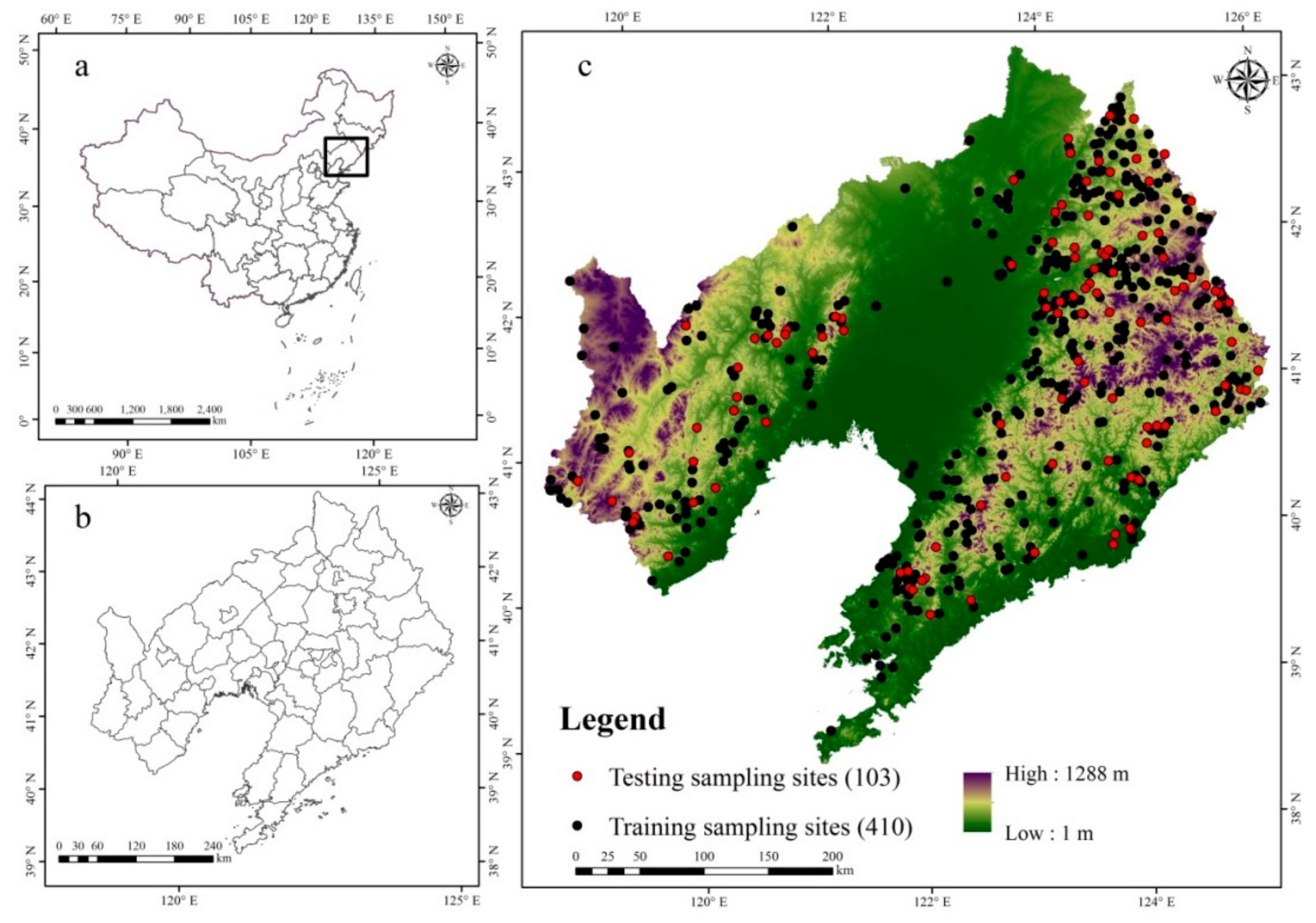
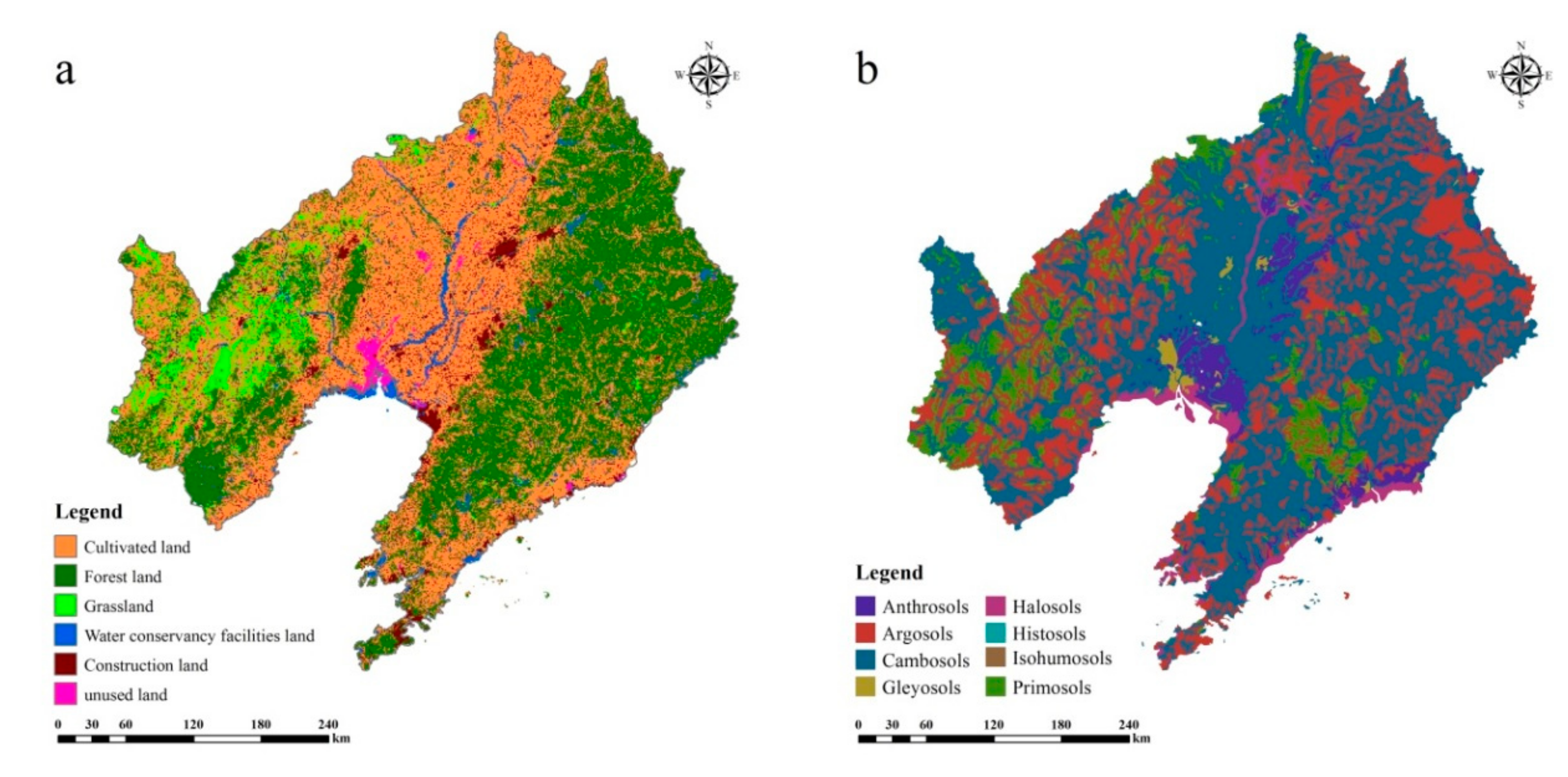
2.1. Study Area

Liaoning Province (38°43′- 43°26′N, 38°43′- 43°26′N) is located in the south of northeastern China (Figure 1), with a total area of 148,000 km² [9]. The main land use types are cultivated land, forest land, grassland, construction land, water conservancy facility land, and unused land, accounting for 43.5%, 42.4%, 2.2%, 0.6%, 1%, and 9.3% of the total area, respectively (Figure 2a). The altitude ranges from 1 m in the southwest of the coastal area to 1288 m in the northeastern mountainous area. The terrain is generally reduced from north to south and inclines from east to west to the middle. The study area had a continental monsoon climate in the North Temperate Zone with four distinct seasons. The annual average precipitation is 400–1100 mm, and 65–75% is concentrated from June to August, accompanied by heavy rain. The annual average temperature ranges from 7 ℃ to 11 ℃, with the highest temperature of 30 ℃ in summer and the lowest temperature of −40 ℃ in winter.

According to the soil system classification of China, the dominant soil types covering the whole study area are Cambosols and Argosols [9], followed by Primosols, Anthrosols, Halosols, Gleyosols, Isohumosols, and Histosols, accounting for 54.44%, 27.72%, 10.34%, 4.07%, 2.53%, 0.79%, 0.10%, and 0.01%, respectively (Figure 2b). Cambosols is a soil with cambic horizon. The main process of its formation is the low degree of mineralization and leaching of base ions. This type of soil is widely distributed in the whole region (Figure 2b). The variation of SOC content in Cambosols is large, and affected by soil parent material. Argosols refers to the soil with obvious clay particles and fully leached lime under the condition of moist soil moisture. Its clay content is high, and it is composed of silicate clay mineral which is not completely weathered. Its texture is relatively sticky, mostly in the form of prismatic block structure, with brown glue film. The SOC content in Argosols is relatively high (20–40 g kg⁻¹ in the topsoil layer) [9]. This type of soil is mainly distributed in the middle Liaohe alluvial plain area in our study region. Primosols is a kind of young soil and its soil properties basically keep the characteristics of soil parent material, with only an ochric epipedon, which is widely distributed in the river banks, estuarine deltas, alluvial plains and sand accumulation areas. Its existence is closely related to the short soil forming time, extreme drought, cold climate, high quartz content with strong weathering resistance, continuous soil erosion and accumulation, and artificial disturbance, so its SOC content is relatively low. Anthrosols is a new kind of soil type. Its original soils have changed through cultivation, fertilization, irrigation and drainage due to human activities. This type of soil is mainly distributed in the middle of Liaoning Province. This area is the main farming area of Liaoning Province, with frequent and intense human activities. Gleyosols, Isohumosols, and Histosols are relatively less distributed in Liaoning Province, but they have the highest SOC content.

2.2. Data Sources

2.2.1. Soil Sampling Collection and Measurement

Field intensive sampling is a time and money consuming activity, especially for a large forest area. In order to accurately reflect the spatial heterogeneity of SOC and STN stocks in those regions, a purposeful sampling method [26] was used. First, we selected main environmental factors that affect the spatial variability of topsoil SOC and STN, including mean annual precipitation, mean annual temperature, elevation, slope gradient, and slope aspect. In addition, we also recognized that parent material, groundwater and vegetation are important environmental factors that determine the spatial variation of SOC and STN [10,15,21,26]. However, it was difficult to obtain them in this study. Consequently, we only used soil type map, topographic wetness index and normalized difference vegetation index (NDVI) to approximate their characterization at sampling sites. Second, a fuzzy c-means clustering method was used to cluster the whole research area and generated 64 clustering units. Finally, combining with road network information, 8–10 soil samples were collected in each cluster unit and a total of 513 topsoil (0–30 cm) samples were collected in 2015. Meanwhile, we also recorded gravel content greater than 2 mm for later calculation of SOC and STN density. Among all these samples, 80% of the samples were randomly selected as a training dataset, and the remaining 20% of the samples were used as an independent dataset to test the prediction performance of the three models. Limited by funds and personnel, it was very difficult to sample deeper, in such a large region. In our next research, we plan to select a relatively small forest area to carry out deeper sampling so as to obtain more accurate SOC and STN stocks of forest soils. In addition, 100 cm³ of undisturbed soil cores were collected from the topsoil layer for subsequent laboratory determination of soil bulk density. The longitude and latitude information of each sample site was recorded by a hand-held GPS, and the positioning accuracy was 5 m.

SOC and STN contents were measured using a dry combustion method and a Vario EL III elemental analyzer in the Central Laboratory at Shenyang Agricultural University. The 100 cm³ core samples were dried in an oven at 105 ℃ for 48 hours to determine the soil bulk density. SOC and STN stocks were calculated using the following formulas:

$$SO{C}_{density}={\displaystyle \sum _{i=1}^{k}SO{C}_{content}}\times B{D}_i\times D_i\times \left(1-S_i\right)$$

(1)

$$ST{N}_{density}={\displaystyle \sum _{i=1}^{k}ST{N}_{content}}\times B{D}_i\times D_i\times \left(1-S_i\right)$$

(2)

where SOC_density and STN_density are the SOC and STN density at i soil layer (kg m⁻²), respectively; SOC_content and STN_content are the SOC and STN contents (g kg⁻¹), respectively; BD_i is the soil bulk density (g cm⁻³); D_i and S_i are the soil layer thickness (m) and the gravel content greater than 2 mm (%), respectively; i is specific soil layer, in this study, it represents topsoil 30 cm; k represents the number of sampling sites.

2.2.2. Remote Sensing Related Data

In this study, the remote sensing data were obtained from Landsat 8 satellite, downloaded from the United States Geological Survey (USGS). We obtained 11 satellite images from July to September of 2015, with cloud cover less than 10%. In MATLAB software, we used a homomorphic filtering method [27] to remove the cloud from the remote sensing images. The spatial resolution of the remote sensing data was 30 meters, and the data level was L1T, which went through geometric precision correction. Therefore, it was not necessary to use the ground control points or digital elevation model (DEM) data to do geometric precision correction again. In addition, many previous studies have shown that the Bottom-Of-Atmosphere (BOA) reflectance is the most appropriate remote sensing variable to predict the spatial distribution of SOC and STN [28]. However, to obtain the BOA reflectance, atmospheric correction shall be performed for the remote sensing data. In this study, we used the Fast Line-of-sight Atmospheric Analysis of Spectral Hypercubes (FLAASH) atmospheric correction method [29] to calibrate the atmosphere in Environment for Visualizing Images (ENVI) 5.1 software. Due to the sun’s altitude angle, some remote sensing images appeared to have mountain shadow, so we used a ratio method [12] to eliminate it in ENVI 5.1 software. Furthermore, we also carried out topographic correction because the study region is a mountainous area. We used a cosine correction method for the topographic correction of remote sensing images [30]. This method is based on the modeling of illumination (IL) condition, so a DEM with the same spatial resolution as Landsat 8 images was needed. Subsequently, the IL conditions were modeled using the ground slope and aspect, as well as solar and satellite parameters. DEM is required to calculate the incident angle (${\lambda }_i$), defined as the angle perpendicular to the ground and the sun light. The IL parameter is between −1 and +1, indicating the minimum and maximum illuminance, respectively, which can be calculated with Equation (3):

$$IL=\cos {\lambda }_i=\cos {\phi }_p\cos {\phi }_z+\sin {\phi }_p\sin {\phi }_z\left({\varphi }_a-{\varphi }_b\right)$$

(3)

where ${\phi }_p$ is the slope angle; ${\phi }_z$ is the solar zenith angle; ${\varphi }_a$ is the solar azimuth angle; and ${\varphi }_b$ is the aspect angle. In the cosine correction method, the reflectance of the surface is calculated using Equation (4):

$${\rho }_h={\rho }_t\left(\frac{\cos {\theta }_z}{IL}\right)$$

(4)

where ${\rho }_h$ is the surface reflectance; ${\rho }_t$ is the reflectance of an inclined surface; and ${\theta }_z$ is the solar zenith angle. This method does not require any external parameters.

Then, the region of interest (ROI) (forest boundary vector layer which was obtained from Liaoning Provincial Department of Natural Resources, China) was used to cut the remote sensing imagery data, remove the overlapped parts, and then to assemble the multiple images to form a mosaic of the region. The selected remote sensing data with 9 variables, included Landsat TM green band reflectance (B_GREEN), Landsat TM red band reflectance (B_RED), Landsat TM near-infrared band reflectance (B_NIR), difference vegetation index (DVI), enhanced vegetation index (EVI), ratio vegetation index (RVI), normalized difference vegetation index (NDVI), renormalization difference vegetation index (RDVI), and soil adjusted vegetation index (SAVI). B_GREEN, B_RED, and B_NIR represent the growth and biomass of vegetation, respectively, and the ground feature images are rich, clear and well-organized [15,21]. In the field of remote sensing science, NDVI is widely used in crop growth monitoring and yield prediction and serves as the best indicator of vegetation growth [31]. SAVI explains the change in optical characteristics of the background [32]. Different from NDVI, SAVI introduces a soil-adjusted coefficient to modify NDVI, which mainly reflects the influence of soil background on vegetation coverage, and its value ranges from 0 to 1. When SAVI is 0, vegetation coverage is 0; when SAVI is 1, the influence of soil background value is 0, mainly indicating that the influence of soil background is 0 in areas with dense canopy. Huete’s research [33], conducted in a well-vegetated area, found that when the coefficient of soil adjusted L is 0.5, SAVI had a better effect on eliminating soil reflectance. RVI can better reflect the difference of vegetation coverage and growth status, especially suitable for vegetation monitoring with vigorous growth and high coverage [34]. DVI, proposed by Richardson et al. [35], is very sensitive to the change of soil background. It can be used to identify water bodies well, and it increases rapidly with an increase in vegetation. RDVI increases rapidly with the increase of vegetation coverage when the vegetation is within the middle and low coverage, and increases slowly when the vegetation reaches certain coverage. So RDVI is suitable for monitoring the early and middle growth stages of vegetation [36]. The specific definitions of these indices are:

$$SAVI=\left(B_{NIR}-B_{RED}\right)\left(1+L\right)/\left(B_{NIR}+B_{RED}+L\right) \mathrm{L}=0.5$$

(5)

$$NDVI=\left(B_{NIR}-B_{RED}\right)/\left(B_{NIR}+B_{RED}\right)$$

(6)

$$RVI=B_{RED}/B_{NIR}$$

(7)

$$DVI=2.4B_{NIR}-B_{RED}$$

(8)

$$RDVI=\sqrt{NDVI\times DVI}$$

(9)

$$EVI=\frac{2.5\left(B_{NIR}-B_{RED}\right)}{\left(B_{NIR}+6B_{RED}-7.5B_{BLUE}+1\right)}$$

(10)

where B_NIR, B_RED, and B_BLUE represented Landsat TM near-infrared band reflectance, Landsat TM red band reflectance, and Landsat TM blue band reflectance, respectively; L is the coefficient of soil adjusted, and its value range is from 0 to 1. In this study, we set it to 0.5.

2.3. Prediction Models

2.3.1. Geographically Weighted Regression

Geographically weighted regression (GWR), multiple stepwise linear regressions (MSLR), and boosted regression trees (BRT) models were compared to obtain the best prediction of SOC and STN stocks in the forest area. GWR is the most classical spatial analysis technology and has been widely used in geographic science and spatial analysis [22]. GWR could be used for prediction by establishing a local regression equation at each point in space [37]. Because it considers the local effect of spatial objects, its advantage is of high accuracy. GWR is developed on the basis of the least square (OLS) model. The basic assumption of OLS is that the direct relationship between independent variables and dependent variables in a region is stable and uniform. In the OLS model, the regression coefficient of the model is for the whole research area and is calculated as an average value, which does not reflect the spatial characteristics of the regression parameters [38]. To overcome this problem, a spatial variable parameter regression model was used [39]. The parameters in the global model are a function of geographical location, so the change trend of parameters in space can be measured [22]. GWR is an extension of ordinary linear regression model, which embeds the spatial position of data into regression [37]. The GWR model was expressed as:

$$Y(i)={\xi }_o({\upsilon }_i,{\delta }_i)+{\displaystyle \sum _k{\xi }_k}({\upsilon }_i,{\delta }_i)x_{i,k}+{\varpi }_i$$

(11)

where (ν_i, δ_i) are the coordinates for the i location; ξ_o (ν_i, δ_i), is the intercept, ξ_k is a regression coefficient, and x_i,k is an environmental variable at the i location, and k is the number of environmental variables. The regression parameters of this equation are estimated at each location i (ν_i, δ_i). ω_i is the residual values at i point. In this study, we used the “spgwr” package [22] in R software environment.

2.3.2. Multiple Stepwise Linear Regressions

As a classical prediction method, MLSR is widely used to predict soil properties and the interaction between analysis variables by considering many factors [40,41]. For instance, Ishii et al. [42] used the MLSR method by considering all relevant information, eliminating irrelevant factors, simplifying equations, reducing errors, adding variables to the model one by one, and analyzing the explanatory variables with F-test. The MLSR model introduced each variable into the model one by one, and F-test was used to analyze and explain the contribution of each variable to the prediction [43]. In the process of modeling, environment variables were introduced into the model one by one, and unimportant environment variables were proposed by using t-test [41]. During the whole iteration process, the iteration was stopped until there were no environment variables that could be added and deleted in the modeling process. Therefore, the final model only included the important environmental variables that affected the spatial distribution of soil attributes. The MLSR models can be expressed as:

$$SO{C}_{density}=12.73-(0.87\pm 0.07)*B_{GREEN}+(0.46\pm 0.06)*SAVI-(0.43\pm 0.03)*RVI+(0.23\pm 0.03)*EVI$$

(12)

$$ST{N}_{density}=1.39-(0.18\pm 0.02)*B_{GREEN}+(0.26\pm 0.04)*SAVI-(0.28\pm 0.05)*RVI+(0.14\pm 0.03)*EVI$$

(13)

R² values of Equations (12) and (13) were 0.46 and 0.41, respectively, while the errors were 9.32 kg m⁻² (±0.52) for SOC stocks and 1.26 kg m⁻² (±0.31) for STN stocks.

2.3.3. Boosted Regression Trees

BRT model was developed by Friedman et al. [44]. It is composed of boosting and regression trees [15]. Based on the random gradient of decision tree, boosting technology introduces all samples into the model at one time, and corrects the model by constantly changing the weight. In the process of multiple iterations, the goal of the next iteration is to find a function to fit the residuals of the previous round. The iteration can only be stopped when the residuals are small enough or when they reach the number set by the user [9]. BRT models can easily deal with soil environment problems in complex landscape areas, and avoid nonlinear and interaction problems [15]. Compared with the traditional regression model, the BRT model has better prediction performance, especially in the spatial prediction of soil properties (such as SOC, STN, and pH) [9]. In this study, we used the "gbm" software package developed by Elith et al. [45] to build the model in the R language environment. The fitting of BRT model was controlled by four parameters: Learning rate (LR), tree complexity (TC), bag fraction (BF), and tree number (NT) [46]. LR represents the contribution of each tree in the model to the final fit model. TC is a direct predictor of tree depth and maximum interaction level [21]. BF represents the scale of data used in each model [9]. NT is determined by LR and TC [15]. To obtain the best prediction performance of the BRT model, we tested different combinations of LR (0.0025, 0.025, 0.25, and 0.50), TC (3, 6, 8, 9 and 10), BF (0.45–0.75) and NT (500, 800, 1000, 1200, and 1500) through 10-fold cross-validation technology. Finally, we found the model has the smallest error when LR, TC, BF and NT are 0.025, 9, 0.65 and 1200, respectively.

2.4. Prediction Accuracy

Randomly selected, 80% of the total samples were used as model training data (n = 410), and the remaining 20% for model validation and accuracy assessment (n = 103). The mean absolute error (MAE), the root mean square error (RMSE), the coefficient of determination (R²) and the concordance correlation coefficient (LCCC) [47] were selected to test the performance of the GWR, MLSR and BRT models. Previous studies [44,47] have revealed that error estimation is an effective method to test different models and datasets. The specific indices used for the validation were:

$$MAE=\frac{1}{n}{\displaystyle \sum _{i=1}^n\left|Y_i-X_i\right|}$$

(14)

$$RMSE=\sqrt{\frac{1}{n}{\displaystyle \sum _{i=1}^n{\left(Y_i-X_i\right)}^2}}$$

(15)

$$R^2=\frac{{\displaystyle \sum _{i=1}^n{\left(Y_i-{\overline{X}}_i\right)}^2}}{{\displaystyle \sum _{i=1}^n{\left(Y_i-{\overline{X}}_i\right)}^2}}$$

(16)

$$LUCC=\frac{2r{\partial }_Y{\partial }_X}{{\partial }_Y^2+{\partial }_X^2+{\left(\overline{Y}+\overline{X}\right)}^2}$$

(17)

where Y and X represent the predicted value and measured value at sampling point i; $\overline{Y}$ and $\overline{X}$ represent the average value of the predicted value and measured value at sampling sites; ${\partial }_Y$ and ${\partial }_X$ represent the change of the predicted value and measured value at sampling point; n represents the number of samples; r represents the Pearson correlation coefficient.

3. Results

3.1. Exploratory Data Analysis

Table 1. Summary statistics of topsoil (0–30 cm) soil organic carbon (SOC) stocks (kg m⁻²), soil total nitrogen (STN) stocks (kg m⁻²), and remote sensing environment variables at sample sites.

Property	Min.	Median	Mean	Max.	SD	Skewness	Kurtosis
SOC stocks	0.23	9.32	10.32	30.23	0.53	0.54	2.31
STN stocks	0.13	1.15	1.21	2.96	0.32	0.63	3.12
BGREEN	0.09	0.14	0.16	0.37	0.17	0.54	1.65
BRED	0.18	0.34	0.35	0.50	0.21	0.32	1.72
BNIR	0.18	0.40	0.41	0.63	0.24	0.48	1.83
SAVI	0.16	0.41	0.44	0.76	0.24	−0.41	1.87
NDVI	0.13	0.39	0.41	0.72	0.22	−0.38	1.75
RVI	1.65	2.29	2.78	4.12	1.16	−1.13	1.23
DVI	65.31	135.33	136.21	193.11	24.51	0.04	2.24
EVI	0.18	0.59	0.60	0.95	0.33	−0.58	2.51
RDVI	72.44	138.61	143.21	201.43	26.41	0.62	3.13

Note: B_GREEN, Landsat TM green band reflectance; B_RED, Landsat TM red band reflectance; B_NIR, Landsat TM near-infrared band reflectance; SAVI, soil adjusted vegetation index; NDVI, normalized difference vegetation index; RVI, ratio vegetation index; DVI, difference vegetation index; EVI, enhanced vegetation index; RDVI, renormalization difference vegetation index.

listed the descriptive statistics of the measured topsoil (0–30 cm) SOC and STN stocks, and remote sensing environment variables at sample sites. The average SOC and STN stocks of topsoils were 10.32 kg m⁻² (±0.53) and 1.21kg m⁻² (±0.32), respectively. Under the generalized skew distribution with skew coefficients of 0.54 and 0.63, the measured topsoil SOC and STN stocks can be well described in this area. Histosols (the average SOC and STN stocks were 13.14 kg m⁻² and 1.43 kg m⁻², respectively) and Isohumosols (the average SOC and STN stocks were 10.71 kg m⁻² and 1.37 kg m⁻², respectively) have the highest SOC and STN stocks, while Primosols (the average SOC and STN stocks were 4.32 kg m⁻² and 0.93 kg m⁻², respectively) has the lowest SOC and STN stocks in 2015 (

Table 2. Summary statistics of topsoil (0–30 cm) soil organic carbon (SOC) stocks (kg m⁻²) and soil total nitrogen (STN) stocks (kg m⁻²) of each soil group according to the Chinese soil system classification at sampling sites.

Property	Soil Groups	Number	Min.	Median	Mean	Max.	SD	Skewness	Kurtosis
SOC stocks	Argosols	154	0.49	9.86	10.38	26.16	0.54	0.57	2.41
	Cambosols	148	0.44	8.84	9.30	22.41	0.47	0.47	2.21
	Gleyosols	23	0.26	5.36	5.58	13.67	0.43	0.52	2.14
	Halosols	43	0.23	4.62	4.86	11.23	0.37	0.43	1.95
	Histosols	27	0.62	12.48	13.14	30.23	0.49	0.55	2.17
	Isohumosols	29	0.5	10.39	10.71	28.38	0.38	0.49	1.87
	Primosols	89	0.23	4.1	4.32	10.02	0.36	0.41	1.72
STN stocks	Argosols	154	0.26	1.32	1.35	2.47	0.35	0.68	3.23
	Cambosols	148	0.23	1.17	1.23	2.25	0.27	0.59	2.75
	Gleyosols	23	0.22	1.06	1.14	1.97	0.25	0.52	2.17
	Halosols	43	0.19	0.97	1.02	1.66	0.22	0.47	2.83
	Histosols	27	0.27	1.39	1.43	2.96	0.32	0.63	2.95
	Isohumosols	29	0.26	1.3	1.37	2.53	0.29	0.54	1.98
	Primosols	89	0.13	0.89	0.93	1.27	0.23	0.52	2.03

Note: Min., minimum; Max., maximum; SD, standard deviation.

).

The correlation coefficients between topsoil SOC and STN stocks, and selected remote sensing environmental variables are shown in

Table 3. Pearson correlation coefficient between observed topsoil (0–30 cm) SOC and STN stocks (kg m⁻²) and all remote sensing environmental variables at sample sites.

Property	SOC Stocks	STN Stocks	BGREEN	BRED	BNIR	SAVI	NDVI	RVI	DVI	EVI
STN stocks	0.65 **
BGREEN	−0.53 **	−0.43 **
BRED	0.21 *	0.13	−0.39 **
BNIR	−0.36 **	−0.29 **	0.61 **	0.14
SAVI	0.45 **	0.34 **	−0.53 **	0.33 **	−0.41 **
NDVI	0.56 **	0.45 **	−0.65 **	0.57 **	−0.39 **	0.73 **
RVI	−0.18 *	−0.23 *	−0.22 *	0.39 **	−0.29 **	−0.22 **	−0.26 **
DVI	0.26 *	0.34 **	0.16 *	−0.28 **	0.43 **	0.17 *	0.29 **	−0.33 **
EVI	0.39 **	0.32 **	0.15 *	−0.09	0.32 **	−0.25 **	−0.35 **	−0.24 **	0.37 **
RDVI	−0.35 **	−0.25 *	−0.07	0.17	−0.18 *	0.43 **	0.46 **	−0.08	0.41 **	0.26 **

Note: p < 0.05 shown in “*”; p < 0.01 shown in “**”. B_GREEN, Landsat TM green band reflectance; B_RED, Landsat TM red band reflectance; B_NIR, Landsat TM near-infrared band reflectance; SAVI, soil adjusted vegetation index; NDVI, normalized difference vegetation index; RVI, ratio vegetation index; DVI, difference vegetation index; EVI, enhanced vegetation index; RDVI, renormalization difference vegetation index.

. SOC and STN stocks were negatively correlated with B_GREEN, B_NIR, and RDVI, and positively correlated with SAVI, NDVI and EVI. We found that there was a multicollinearity between the environmental variables of remote sensing data (Table 3). It was not reliable to use a simple linear method to predict topsoil SOC and STN stocks in space. Comparing multiple, more sophisticated models helps identify the best model and obtain accurate spatial distribution of topsoil SOC and STN stocks.

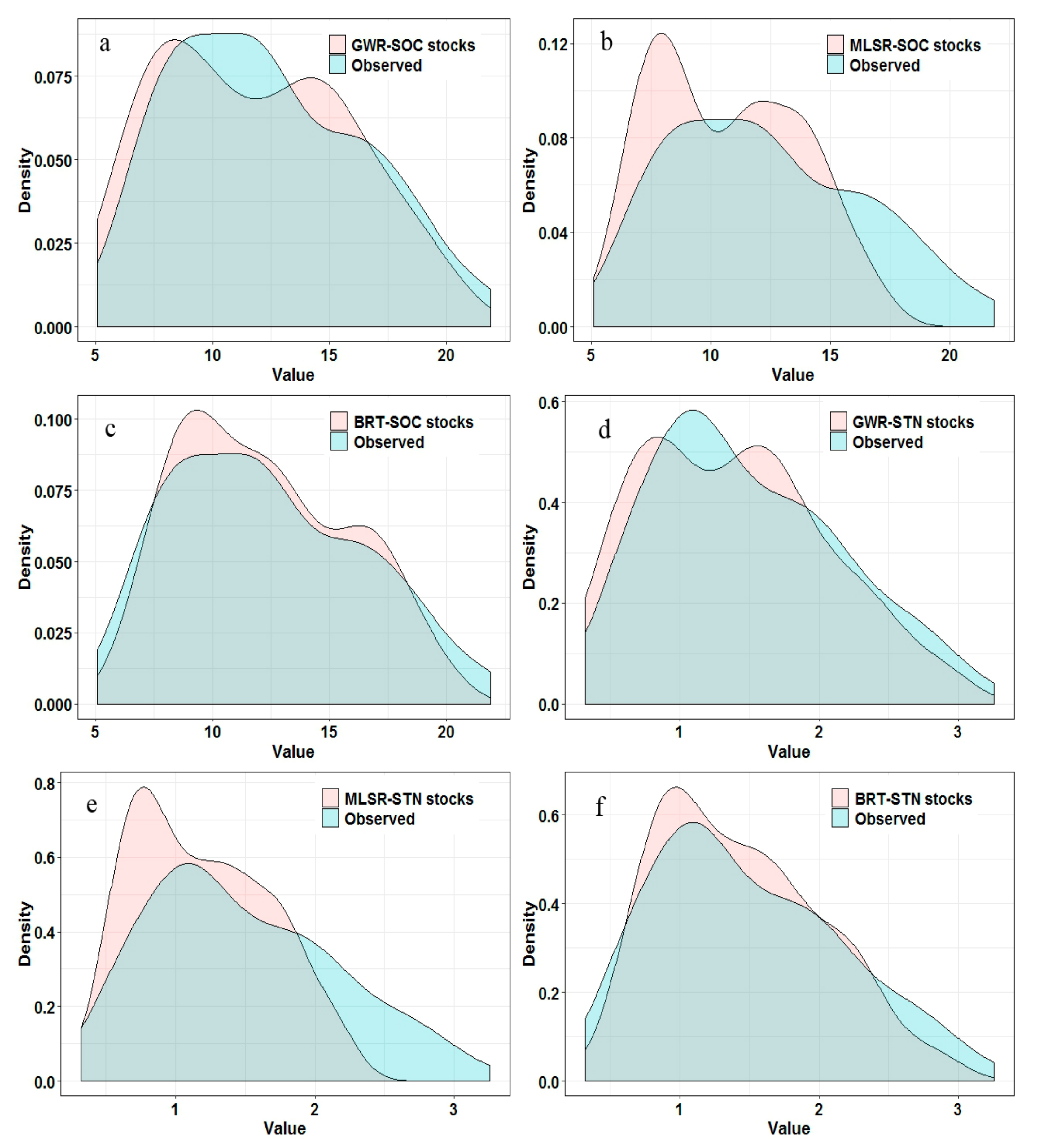
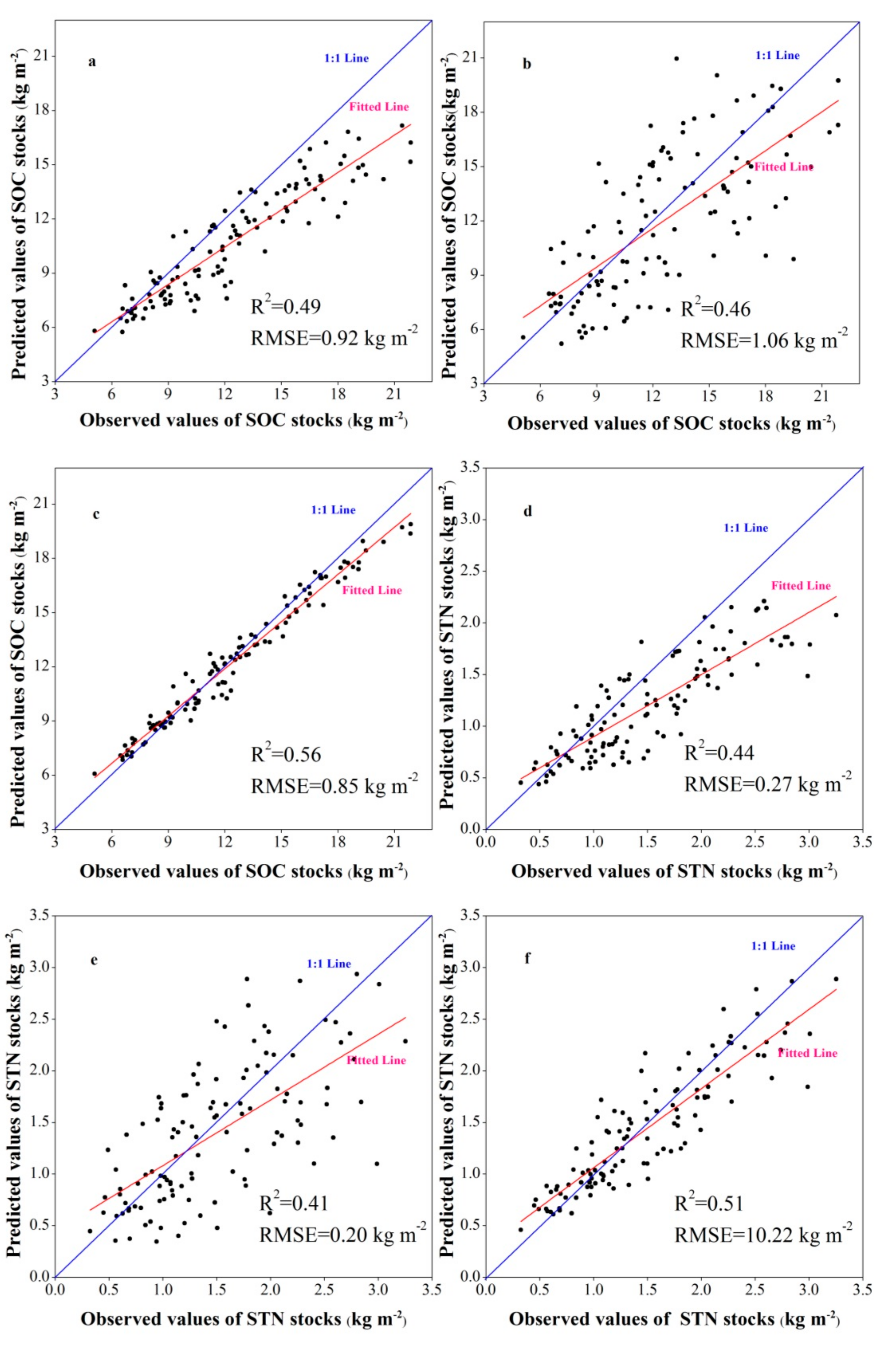
3.2. Model Performance and Uncertainty

In forest ecosystems in northeastern China, the spatial prediction performance of GWR, MLSR and BRT models for topsoil SOC and STN stocks was compared. The summary statistical results of model validation are shown in

Table 4. Summary statistics of the predictive quality of geographically weighted regression (GWR), multiple stepwise linear regression (MSLR), and boosted regression trees (BRT) for topsoil (0–30 cm) SOC and STN stocks based on an independent dataset (n = 103) in 2015.

Property	Model	Index	Min.	Median	Mean	Max.
SOC stocks	GWR	MAE	0.82	0.84	0.84	0.90
		RMSE	0.89	0.91	0.92	0.95
		R2	0.48	0.49	0.49	0.51
		LCCC	0.60	0.61	0.61	0.66
	MLSR	MAE	0.82	0.84	0.84	0.89
		RMSE	1.02	1.04	1.06	1.08
		R2	0.45	0.45	0.46	0.48
		LCCC	0.58	0.62	0.64	0.68
	BRT	MAE	0.66	0.70	0.71	0.75
		RMSE	0.82	0.84	0.85	0.88
		R2	0.53	0.56	0.56	0.58
		LCCC	0.77	0.78	0.80	0.82
STN stocks	GWR	MAE	0.15	0.16	0.16	0.19
		RMSE	0.26	0.27	0.27	0.31
		R2	0.39	0.42	0.44	0.45
		LCCC	0.47	0.47	0.47	0.50
	MLSR	MAE	0.18	0.19	0.19	0.20
		RMSE	0.17	0.19	0.20	0.22
		R2	0.39	0.40	0.41	0.43
		LCCC	0.42	0.44	0.45	0.47
	BRT	MAE	0.16	0.16	0.16	0.17
		RMSE	0.20	0.22	0.22	0.25
		R2	0.47	0.50	0.51	0.54
		LCCC	0.63	0.64	0.65	0.65

Note: MAE, the mean error; RMSE, root mean squared error; R² coefficient of determination; LCCC, Lin’s concordance correlation coefficient are used to evaluate accuracy; Min., minimum; Max., maximum.

. Comparing the three models in topsoil SOC and STN stock prediction performance, BRT was the best, followed by GWR and MLSR models. The BRT model with the best performance could explain the spatial variation of 56% and 51% SOC and STN stocks in the region, respectively. To further examine the three models, we created density plots of the predicted and measured values of SOC and STN stocks at the sampling sites (Figure 3). We also presented scatter plots of the predicted and measured values, which also indicated that the BRT model has the best performance (Figure 4). Overall, BRT performs the best, matching with the measured topsoil SOC and STN stocks. We iterated the BRT model 100 times and calculated the average standard deviation (SDs) to analyze the uncertainty of the BRT model in predicting topsoil SOC and STN stocks (Figure 5). We found that the BRT model had a lower uncertainty compared with GWR and MLSR models.

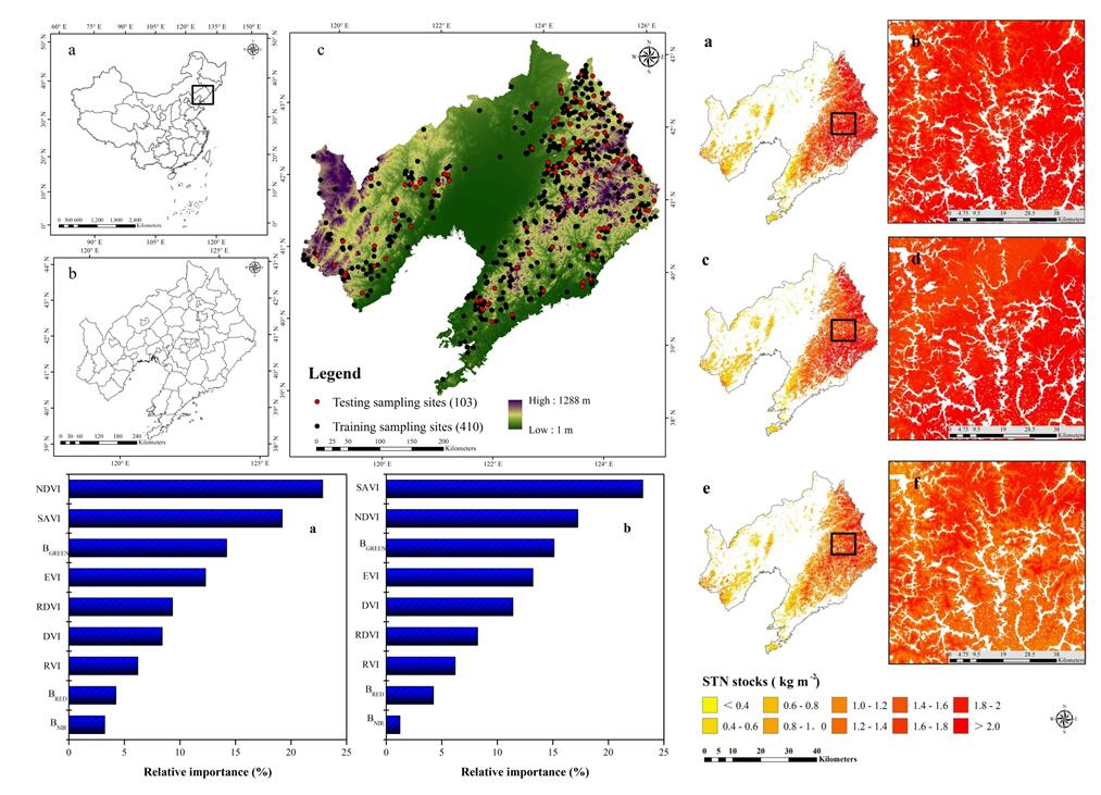
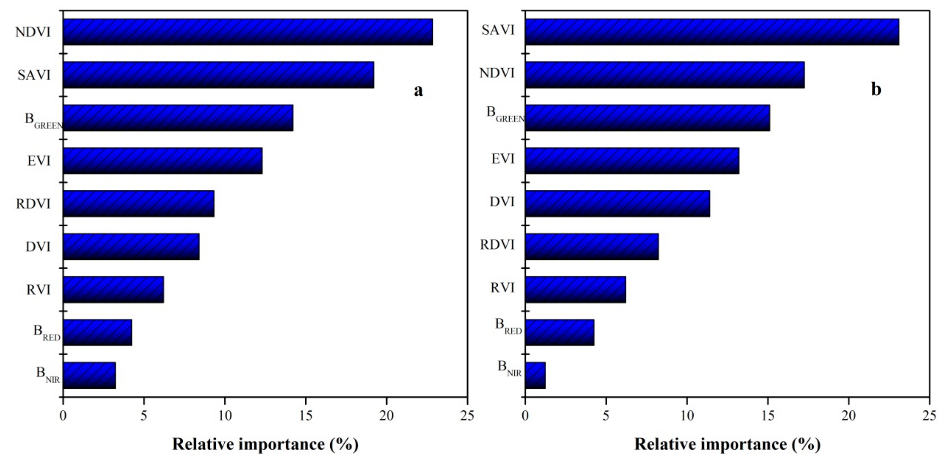
3.3. Importance of Remotely Sensed Environmental Variables

Through 100 iterations of BRT model, the average relative importance of each remotely-sensed environmental variable in predicting topsoil SOC and STN stocks was calculated. To facilitate the analysis of the model, we combined the relative importance of all environments to 100% (Figure 6). We found that the main remotely-sensed environmental variables affecting the spatial variability of topsoil SOC stocks were NDVI, SAVI, B_GREEN, EVI, and RDVI (77% of the total relative importance). Correspondingly, SAVI, NDVI, B_GREEN, EVI and DVI were the main environmental variables (accounting for 80% of the total relative importance) that affect the spatial variability of topsoil STN stocks in forest dominated areas.

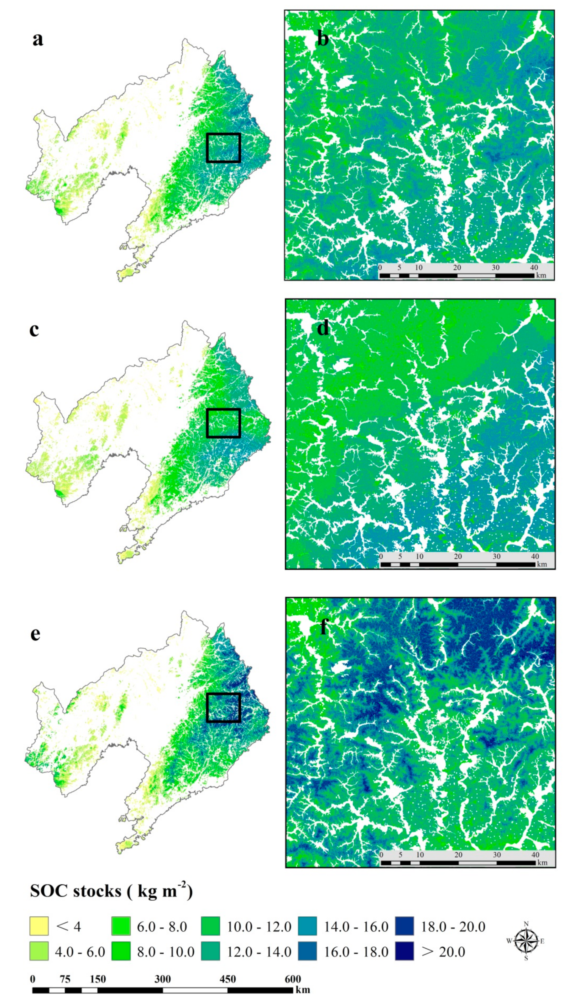
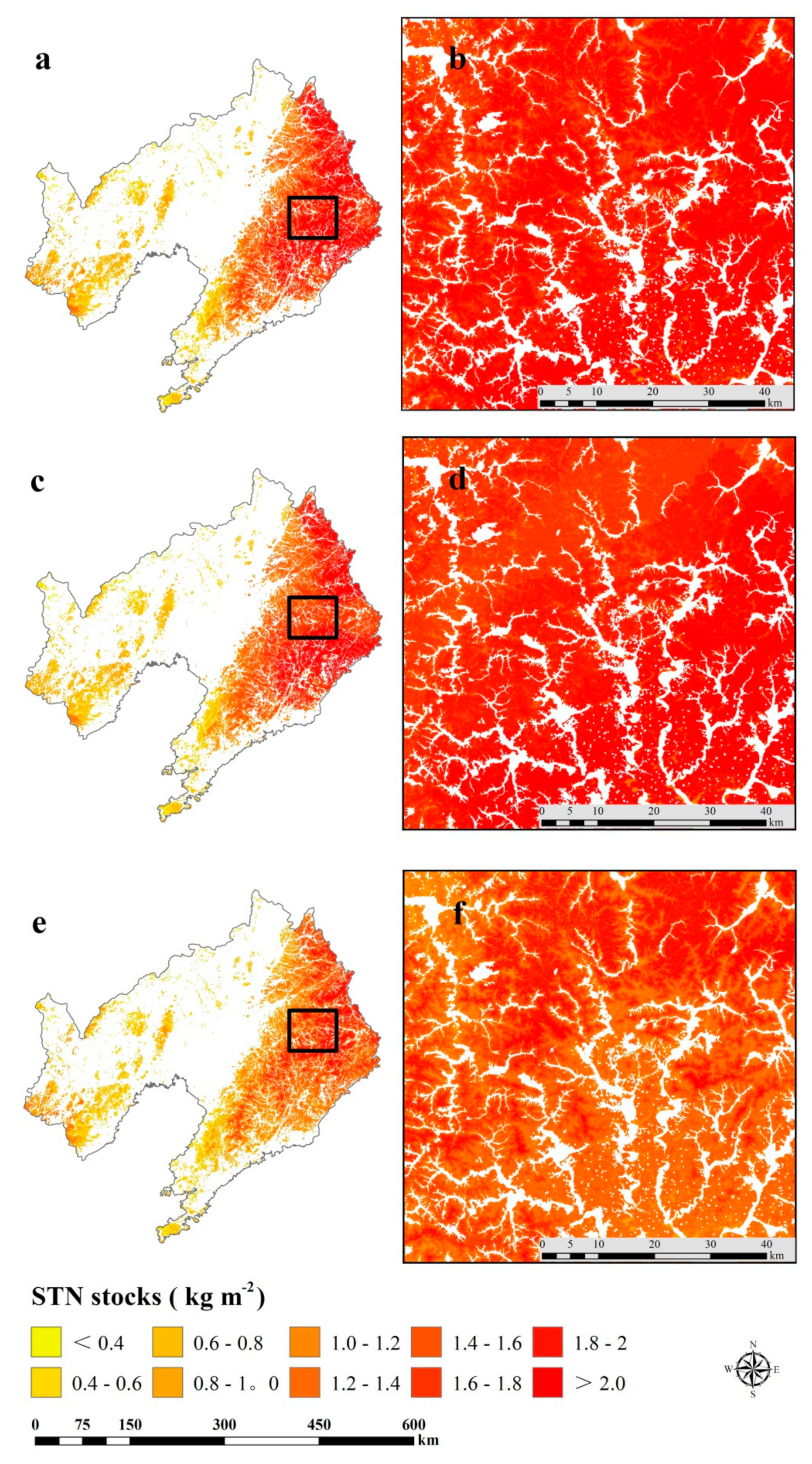
3.4. Spatial Prediction of SOC and STN Stocks

Our model verification showed that BRT model performs best, so it was selected as the final model to predict the spatial distribution of topsoil SOC and STN stocks (

Table 5. Statistical description of soil organic carbon (SOC) and soil total nitrogen (STN) stocks of each soil groups according to the Chinese soil system classification estimated with boosted regression model (BRT) in forest topsoil (0–30 cm).

Soil Groups	Area (km2)	Average SOC Stocks (kg m−2)	Average STN Stocks (kg m−2)	SOC Stock (Tg)	STN Stock (Tg)
Argosols	5486.00	3.46	0.45	19.01	2.46
Cambosols	43959.00	2.92	0.49	128.35	21.54
Gleyosols	233.00	1.72	0.37	0.40	0.09
Halosols	774.00	1.51	0.32	1.17	0.25
Histosols	13.00	4.13	0.35	0.05	0.01
Isohumosols	12.00	3.57	0.40	0.04	0.01
Primosols	12275.00	1.36	0.29	16.68	3.61
Sum	62752.00			165.69	27.96

). The topsoil SOC and STN were mainly stored in Argosols and Cambosols in forest ecosystems Liaoning Province, accounting for 88.9% and 85.8% of topsoil SOC and STN stocks, respectively. In addition, the BRT model showed that topsoil SOC and STN stocks had a similar spatial distribution pattern (Figure 7 and Figure 8), increasing gradually from southwest to northeast, and the average topsoil SOC stocks increase from 0.51 to 28.12 kg m⁻² estimated with BRT model. Correspondingly, the average topsoil STN stocks increased from 0.22 to 2.73 kg m⁻².

4. Discussion

4.1. Role of Remotely-Sensed Enviroment Variables in Predicting Topsoil SOC and STN Stocks

In forest ecosystems, the combination of remotely-sensed data and BRT model provided a better prediction (Table 3) of SOC and STN stocks in topsoil, which was consistent with previous findings [21,46]. For instance, Chen et al. [48] used remote sensing images to predict the topsoil SOC content of a 115-hectare land in crisp County, Georgia. They found that the remote sensing data showed a significant linear relationship with the topsoil SOC content. Through the study on the semi-arid grassland in eastern Australia, Wang et al. [49] concluded that spatial prediction of SOC stocks was a very challenging task in the semi-arid grassland area, especially in those areas lacking basic data and vegetation coverage. Compared with direct measurement in the field, DSM is an economical method to predict SOC. Previous studies also indicated that the vegetation is correlated with carbon and nitrogen stocks in topsoil [50]. The spectral reflectance of remote sensing data and derived vegetation index reflect vegetation coverage well, which are valuable for mapping SOC and STN.

To compare the contribution of various remotely-sensed environmental variables to the prediction of topsoil SOC and STN stocks, we iterated the BRT model 100 times to calculate their average relative importance, and then merged them into a percentage. We found that NDVI, SAVI and B_GREEN were the most effective variables affecting topsoil SOC and STN stocks in the forest dominated areas. This conclusion was consistent with previous studies. For example, Gong et al. [51] used 8227 soil profiles and a cubist model, a generalized linear model, support vector machines, and random forest models to simulate the SOC stocks in Brazil, by using NDVI as an effective predictor. In the coastal forest area of northeastern China, Qi et al. [52] concluded that SAVI was an important remotely-sensed variable to predict SOC stocks. In the same study area, Wang et al. [21] recommended that SAVI should be introduced into the spatial prediction model of topsoil SOC stocks, especially in dense forest ecosystems. B_GREEN has also been used as an efficient predictor in estimating SOC and STN stocks. According to Yang et al. [53] and Wang et al. [49], B_NIR and B_RED reflected the land-use situation in a region to a certain extent, but our study was limited to the study of SOC and STN stocks of surface forest soils, not all land use types in the region. Therefore, in mapping SOC and STN stocks, B_NIR and B_RED showed the lowest relative importance. DVI could better reflect the difference of vegetation coverage and growth status, especially suitable for vegetation monitoring of dense forests. Similarly, RVI could better reflect the difference of vegetation coverage and growth status, especially suitable for dense forests [54]. DVI was sensitive to the change of soil background and could better identify water bodies. Its value increased with the increase of vegetation density. Therefore, both DVI and RVI were introduced into SOC and STN mapping [55]. Furthermore, in the Jutland peninsula, Denmark, Pouladi et al. [56] used NDVI, SAVI, DVI, RVI and terrain related variables combined with Kriging, cubist model, random forest and regression-Kriging models to predict the SOC content in the topsoil layer. They found these remotely-sensed variables explained the spatial variation of 89% SOC content on average. They also found that, there is no need to introduce other environment variables into the model construction when the sampling sites were dense enough. However, our study suggests that environmental variables including remotely-sensed data are necessary to map these stocks, especially for dense forest areas.

A few studies have also pointed out the importance of using remote sensing data in mapping SOC. For instance, in the coastal forest areas of northeastern China, Wang et al. [46] constructed a BRT model using three multispectral bands, NDVI and SAVI to predict the SOC stocks in topsoil, and achieved high prediction accuracy (R² = 59%). Yang et al. [53] used B_GREEN, B_RED, B_NIR and a random forest model to predict SOC stocks and found that these variables could explain the spatial variation of 72% SOC stocks in this region. In Dalian, China, Wang et al. [15] used three Landsat 5 satellite bands and NDVI data, combining a random forest model, to predict STN content in the topsoil layer. They found that remotely-sensed data should be used as key environmental variables for the prediction in densely forest dominated areas.

4.2. Uncertainty in Current Research

BRT performed best in comparison with GWR and MLSR models to predict SOC and STN in forest areas of northeastern China. However, there were still uncertainties in our prediction. First, data collection and lab analysis were conducted by several groups. Thus, there might be some sampling errors and experimental errors. Second, due to the influence of terrain and clouds, high altitude areas were prone to produce shadows in the process of image segmentation, leading to large reflectivity errors in satellite imagery data. Finally, this study was limited to estimating the SOC and STN stocks of the forest topsoil (0–30 cm), which might lead to underestimation of SOC and STN stocks in the region since SOC and STN are also stored in deep soil layers of forest ecosystems.

5. Conclusions

We used GWR, MLSR and BRT models to estimate the spatial variation of SOC and STN stocks in the forest topsoil of northeastern China. We found that remotely-sensed variables are key to estimating SOC and STN stocks. The BRT model had the best prediction performance in mapping SOC and STN stocks with lower MAE, RMSE and higher R², in comparison with other models. In addition, the estimated SOC and STN stocks show a similar spatial distribution pattern, and gradually increase from southwest to northeast in the region. Among remotely-sensed environment variables, NDVI and SAVI were key factors to predict SOC and STN stocks in forest ecosystems in our study region. We expect our relatively more accurate mapping of SOC and STN shall benefit forest management and climate change policy making in our study region.

References

1. Batjes, N.H. Total carbon and nitrogen in the soils of the world. Eur. J. Soil Sci. 1996, 47, 151–163. [Google Scholar] [CrossRef]
2. Hessen, D.O.; Ågren, G.I.; Anderson, T.R.; Elser, J.J.; De Ruiter, P.C. Carbon sequestration in ecosystems: The role of stoichiometry. Ecology 2004, 85, 1179–1192. [Google Scholar] [CrossRef]
3. Melillo, J.M. Carbon and nitrogen interactions in the terrestrial biosphere: Anthropogenic effects. Glob. Chang. Terr. Ecosyst. 1996, 2, 431. [Google Scholar]
4. Vejre, H.; Callesen, I.; Vesterdal, L.; Raulund-Rasmussen, K. Carbon and nitrogen in Danish forest soils—Contents and distribution determined by soil order. Soil Sci. Soc. Am. J. 2003, 67, 335–343. [Google Scholar] [CrossRef]
5. Lal, R. Forest soils and carbon sequestration. For. Ecol. Manag. 2005, 220, 242–258. [Google Scholar] [CrossRef]
6. Gao, Q.; Guo, Y.; Xu, H.; Ganjurjav, H.; Li, Y.; Wan, Y.; Liu, S. Climate change and its impacts on vegetation distribution and net primary productivity of the alpine ecosystem in the Qinghai-Tibetan Plateau. Sci. Total Environ. 2016, 554, 34–41. [Google Scholar] [CrossRef]
7. Xu, S.; Liu, L.; Sayer, E.J. Variability of above-ground litter inputs alters soil physicochemical and biological processes: A meta-analysis of litterfall-manipulation experiments. Biogeosciences 2013, 10, 7423–7433. [Google Scholar] [CrossRef] [Green Version]
8. Li, C. Quantifying greenhouse gas emissions from soils: Scientific basis and modeling approach. Soil Sci. Plant Nutr. 2007, 53, 344–352. [Google Scholar] [CrossRef] [Green Version]
9. Wang, S.; Zhuang, Q.; Wang, Q.; Jin, X.; Han, C. Mapping stocks of soil organic carbon and soil total nitrogen in Liaoning Province of China. Geoderma 2017, 305, 250–263. [Google Scholar] [CrossRef]
10. McBratney, A.B.; Santos, M.M.; Minasny, B. On digital soil mapping. Geoderma 2003, 117, 3–52. [Google Scholar] [CrossRef]
11. Jenny, H. Factors of Soil Formation; McGraw-Hill: New York, NY, USA, 1941. [Google Scholar]
12. Vermote, E.; Justice, C.; Claverie, M.; Franch, B. Preliminary analysis of the performance of the Landsat 8/OLI land surface reflectance product. Remote Sens. Environ. 2016, 185, 46–56. [Google Scholar] [CrossRef] [PubMed]
13. Martin, M.P.; Wattenbach, M.; Smith, P.; Meersmans, J.; Jolivet, C.; Boulonne, L.; Arrouays, D. Spatial distribution of soil organic carbon stocks in France. Biogeosciences 2011, 8, 1053–1065. [Google Scholar] [CrossRef] [Green Version]
14. Liddicoat, C.; Maschmedt, D.; Clifford, D.; Searle, R.; Herrmann, T.; Macdonald, L.M.; Baldock, J. Predictive mapping of soil organic carbon stocks in South Australia’s agricultural zone. Soil Res. 2015, 53, 956–973. [Google Scholar] [CrossRef]
15. Wang, S.; Jin, X.; Adhikari, K.; Li, W.; Yu, M.; Bian, Z.; Wang, Q. Mapping total soil nitrogen from a site in northeastern China. Catena 2018, 166, 134–146. [Google Scholar] [CrossRef]
16. Duane, M.V.; Cohen, W.B.; Campbell, J.L.; Hudiburg, T.; Turner, D.P.; Weyermann, D.L. Implications of alternative field-sampling designs on Landsat-based mapping of stand age and carbon stocks in Oregon forests. For. Sci. 2010, 56, 405–416. [Google Scholar]
17. Niwa, K.; Yokobori, J.; Hongo, C.; Nagata, O. Estimating soil carbon stocks in an upland area of Tokachi District, Hokkaido, Japan, by satellite remote sensing. Soil Sci. Plant Nutr. 2011, 57, 283–293. [Google Scholar] [CrossRef] [Green Version]
18. Yigini, Y.; Panagos, P. Assessment of soil organic carbon stocks under future climate and land cover changes in Europe. Sci. Total Environ. 2016, 557, 838–850. [Google Scholar] [CrossRef] [PubMed]
19. Mishra, U.; Lal, R.; Slater, B.; Calhoun, F.; Liu, D.; Van Meirvenne, M. Predicting soil organic carbon stock using profile depth distribution functions and ordinary kriging. Soil Sci. Soc. Am. J. 2009, 73, 614–621. [Google Scholar] [CrossRef] [Green Version]
20. Grimm, R.; Behrens, T.; Märker, M.; Elsenbeer, H. Soil organic carbon concentrations and stocks on Barro Colorado Island—Digital soil mapping using Random Forests analysis. Geoderma 2008, 146, 102–113. [Google Scholar] [CrossRef]
21. Wang, S.; Gao, J.; Zhuang, Q.; Lu, Y.; Gu, H.; Jin, X. Multispectral Remote Sensing Data Are Effective and Robust in Mapping Regional Forest Soil Organic Carbon Stocks in a Northeast Forest Region in China. Remote Sens. 2020, 12, 393. [Google Scholar] [CrossRef] [Green Version]
22. Kumar, S.; Lal, R.; Liu, D. A geographically weighted regression kriging approach for mapping soil organic carbon stock. Geoderma 2012, 189, 627–634. [Google Scholar] [CrossRef]
23. Nocita, M.; Stevens, A.; Noon, C.; van Wesemael, B. Prediction of soil organic carbon for different levels of soil moisture using Vis-NIR spectroscopy. Geoderma 2013, 199, 37–42. [Google Scholar] [CrossRef]
24. Yu, D.S.; Shi, X.Z.; Wang, H.J.; Sun, W.X.; Chen, J.M.; Liu, Q.H.; Zhao, Y.C. Regional patterns of soil organic carbon stocks in China. J. Environ. Manag. 2007, 85, 680–689. [Google Scholar] [CrossRef] [PubMed]
25. Roy, D.P.; Wulder, M.A.; Loveland, T.R.; Woodcock, C.E.; Allen, R.G.; Anderson, M.C.; Scambos, T.A. Landsat-8: Science and product vision for terrestrial global change research. Remote Sens. Environ. 2014, 145, 154–172. [Google Scholar] [CrossRef] [Green Version]
26. Zhu, A.X.; Yang, L.; Li, B.; Qin, C.; English, E.; Burt, J.E.; Zhou, C. Purposive sampling for digital soil mapping for areas with limited data. In Digital Soil Mapping with Limited Data; Hartemink, A.E., Ed.; Springer: Berlin/Heidelberg, Germany, 2008; pp. 33–245. [Google Scholar]
27. Liu, Z.K.; Hunt, B.R. A new approach to removing cloud cover from satellite imagery. Comput. Vis. Graph. Image Process. 1984, 25, 252–256. [Google Scholar] [CrossRef]
28. Odebiri, O.; Mutanga, O.; Odindi, J.; Peerbhay, K.; Dovey, S. Predicting soil organic carbon stocks under commercial forest plantations in KwaZulu-Natal province, South Africa using remotely sensed data. GIScience Remote Sens. 2020, 1–14. [Google Scholar] [CrossRef]
29. Perkins, T.; Adlergolden, S.; Matthew, M.; Berk, A.; Anderson, G.; Gardner, J. Retrieval of atmospheric properties from hyper and multispectral imagery with the FLAASH atmospheric correction algorithm. In Remote Sensing of Clouds & the Atmosphere X; International Society for Optics and Photonics: Orlando, FL, USA, 2005. [Google Scholar]
30. Pimple, U.; Sitthi, A.; Simonetti, D.; Pungkul, S.; Leadprathom, K.; Chidthaisong, A. Topographic Correction of Landsat TM-5 and Landsat OLI-8 Imagery to Improve the Performance of Forest Classification in the Mountainous Terrain of Northeast Thailand. Sustainability 2017, 9, 258. [Google Scholar] [CrossRef] [Green Version]
31. Goward, S.N.; Markham, B.; Dye, D.G.; Dulaney, W.; Yang, J. Normalized difference vegetation index measurements from the Advanced Very High Resolution Radiometer. Remote Sens. Environ. 1991, 35, 257–277. [Google Scholar] [CrossRef]
32. Gilabert, M.A.; González-Piqueras, J.; Garcıa-Haro, F.J.; Meliá, J. A generalized soil-adjusted vegetation index. Remote Sens. Environ. 2002, 82, 303–310. [Google Scholar] [CrossRef]
33. Huete, A.R. A soil-adjusted vegetation index (SAVI). Remote Sens. Environ. 1988, 25, 295–309. [Google Scholar] [CrossRef]
34. Richardson, A.J.; Wiegand, C.L. Distinguishing vegetation from soil background information. Photogramm. Eng. Remote Sens. 1977, 43, 1541–1552. [Google Scholar]
35. Major, D.J.; Baret, F.; Guyot, G. A ratio vegetation index adjusted for soil brightness. Int. J. Remote Sens. 1990, 11, 727–740. [Google Scholar] [CrossRef]
36. Payero, J.O.; Neale, C.M.U.; Wright, J.L. Comparison of eleven vegetation indices for estimating plant height of alfalfa and grass. Appl. Eng. Agric. 2004, 20, 385. [Google Scholar] [CrossRef] [Green Version]
37. Brunsdon, C.; Fotheringham, S.; Charlton, M. Geographically weighted regression. R. Stat. Soc. 1998, 47, 431–443. [Google Scholar] [CrossRef]
38. Wang, K.; Zhang, C.; Li, W. Predictive mapping of soil total nitrogen at a regional scale: A comparison between geographically weighted regression and cokriging. Appl. Geogr. 2013, 42, 73–85. [Google Scholar] [CrossRef]
39. Foster, S.A.; Gorr, W.L. An adaptive filter for estimating spatially-varying parameters: Application to modeling police hours spent in response to calls for service. Manag. Sci. 1986, 32, 878–889. [Google Scholar] [CrossRef]
40. Wang, Y.; Zhang, X.; Huang, C. Spatial variability of soil total nitrogen and soil total phosphorus under different land uses in a small watershed on the Loess Plateau, China. Geoderma 2009, 150, 141–149. [Google Scholar] [CrossRef]
41. Lv, J.; Liu, Y.; Zhang, Z.; Dai, J. Factorial kriging and stepwise regression approach to identify environmental factors influencing spatial multi-scale variability of heavy metals in soils. J. Hazard. Mater. 2013, 261, 387–397. [Google Scholar] [CrossRef]
42. Ishii, Y.; Murakami, J.; Sasaki, K.; Tsukahara, M.; Wakamatsu, K. Efficient folding/assembly in Chinese hamster ovary cells is critical for high quality (low aggregate content) of secreted trastuzumab as well as for high production: Stepwise multivariate regression analyses. J. Biosci. Bioeng. 2014, 118, 223–230. [Google Scholar] [CrossRef]
43. Hong, S.Y.; Minasny, H.K.H.; Kim, Y.; Lee, K. Predicting and mapping soil available water capacity in Korea. PeerJ 2013, 1, e71. [Google Scholar] [CrossRef]
44. Friedman, J.; Hastie, T.; Tibshirani, R. Additive logistic regression: A statistical view of boosting. Ann. Stat. 2000, 28, 337–407. [Google Scholar] [CrossRef]
45. Elith, J.; Leathwick, J.R.; Hastie, T. A working guide to boosted regression trees. J. Anim. Ecol. 2008, 77, 802–813. [Google Scholar] [CrossRef] [PubMed]
46. Wang, S.; Zhuang, Q.; Yang, Z.; Yu, N.; Jin, X. Temporal and Spatial Changes of Soil Organic Carbon Stocks in the Forest Area of Northeastern China. Forests 2019, 10, 1023. [Google Scholar] [CrossRef] [Green Version]
47. Lin, L. A concordance correlation coefficient to evaluate reproducibility. Biometrics 1989, 45, 255–268. [Google Scholar] [CrossRef] [PubMed]
48. Chen, F.; Kissel, D.E.; West, L.T.; Adkins, W. Field-scale mapping of surface soil organic carbon using remotely sensed imagery. Soil Sci. Soc. Am. J. 2000, 64, 746–753. [Google Scholar] [CrossRef] [Green Version]
49. Wang, B.; Waters, C.; Orgill, S.; Cowie, A.; Clark, A.; Li Liu, D.; Sides, T. Estimating soil organic carbon stocks using different modelling techniques in the semi-arid rangelands of eastern Australia. Ecol. Indic. 2018, 88, 425–438. [Google Scholar] [CrossRef]
50. Yimer, F.; Ledin, S.; Abdelkadir, A. Soil property variations in relation to topographic aspect and vegetation community in the south-eastern highlands of Ethiopia. For. Ecol. Manag. 2006, 232, 90–99. [Google Scholar] [CrossRef]
51. Gong, Y.; Guo, J.; Li, J.; Zhu, K.; Liao, M.; Liu, X.; Zhang, D. Experimental realization of an intrinsic magnetic topological insulator. Chin. Phys. Lett. 2019, 36, 076801. [Google Scholar] [CrossRef] [Green Version]
52. Qi, L.; Wang, S.; Zhuang, Q.; Yang, Z.; Bai, S.; Jin, X.; Lei, G. Spatial-temporal changes in soil organic carbon and pH in the Liaoning Province of China: A modeling analysis based on observational data. Sustainability 2019, 11, 3569. [Google Scholar] [CrossRef] [Green Version]
53. Yang, R.; Rossiter, D.G.; Liu, F.; Lu, Y.; Yang, F.; Yang, F.; Zhang, G. Predictive mapping of topsoil organic carbon in an alpine environment aided by Landsat TM. PLoS ONE 2015, 10, e0139042. [Google Scholar] [CrossRef]
54. Lu, W.; Lu, D.; Wang, G.; Wu, J.; Huang, J.; Li, G. Examining soil organic carbon distribution and dynamic change in a hickory plantation region with Landsat and ancillary data. Catena 2018, 165, 576–589. [Google Scholar] [CrossRef]
55. Gomez, C.; Rossel, R.A.V.; McBratney, A.B. Soil organic carbon prediction by hyperspectral remote sensing and field vis-NIR spectroscopy: An Australian case study. Geoderma 2008, 146, 403–411. [Google Scholar] [CrossRef]
56. Pouladi, N.; Møller, A.B.; Tabatabai, S.; Greve, M.H. Mapping soil organic matter contents at field level with Cubist, Random Forest and kriging. Geoderma 2019, 342, 85–92. [Google Scholar] [CrossRef]
Figure 1. Soil sampling locations in digital elevation model map (c) at a 30 m spatial resolution in Liaoning Province (b) of China (a).
Remotesensing 12 01115 g001
Figure 2. Land use types (a) and soil types (b) in the study area.
Remotesensing 12 01115 g002
Figure 3. Density plots of the predicted and measured values of topsoil (0–30 cm) soil organic carbon stocks (SOC) (kg m−2) and soil total nitrogen (STN) (kg m−2). The predicted data are derived from geographically weighted regression (GWR) (a,d), multiple stepwise linear regression (MSLR) (b,e), and boosted regression trees (BRT) (c,f).
Remotesensing 12 01115 g003
Figure 4. Scatter plot of the predicted and measured topsoil (0–30 cm) soil organic carbon stocks (SOC) (kg m−2) and soil total nitrogen (STN) (kg m−2). The predicted data are derived from geographically weighted regression (GWR) (a,d), multiple stepwise linear regression (MSLR) (b,e), and boosted regression trees (BRT) (c,f).
Remotesensing 12 01115 g004
Figure 5. Standard deviation of topsoil (0–30 cm) SOC stocks (a) and STN stocks (b) predicted by the boosted regression trees (BRT) model.
Remotesensing 12 01115 g005
Figure 6. Relative importance of remotely-sensed environment variables as determined from 100 iterations using the boosted regression trees (BRT) in predicting topsoil (0–30 cm) SOC stocks (a) and STN stocks (b) in 2015, which are combined into percentage. Note: BGREEN, Landsat TM green band reflectance; BRED, Landsat TM red band reflectance; BNIR, Landsat TM near-infrared band reflectance; SAVI, soil adjusted vegetation index; NDVI, normalized difference vegetation index; RVI, ratio vegetation index; DVI, difference vegetation index; EVI, enhanced vegetation index; RDVI, renormalization difference vegetation index.
Remotesensing 12 01115 g006
Figure 7. Spatial distribution of the predicted topsoil (0–30 cm) soil organic carbon (SOC) stocks with models of geographically weighted regression (GWR) (a,b), multiple stepwise linear regression (MSLR) (c,d), and boosted regression trees (BRT) (e,f).
Remotesensing 12 01115 g007
Figure 8. Spatial distribution of the predicted topsoil (0–30 cm) soil total nitrogen (STN) stocks with models of geographically weighted regression (GWR) (a,b), multiple stepwise linear regression (MSLR) (c,d), and boosted regression trees (BRT) (e,f).
Remotesensing 12 01115 g008