Mapping Heterogeneous Urban Landscapes from the Fusion of Digital Surface Model and Unmanned Aerial Vehicle-Based Images Using Adaptive Multiscale Image Segmentation and Classification

 ,
,  ,
,  ,
, 


Abstract

1. Introduction
Related Studies
2. Study Area and Materials
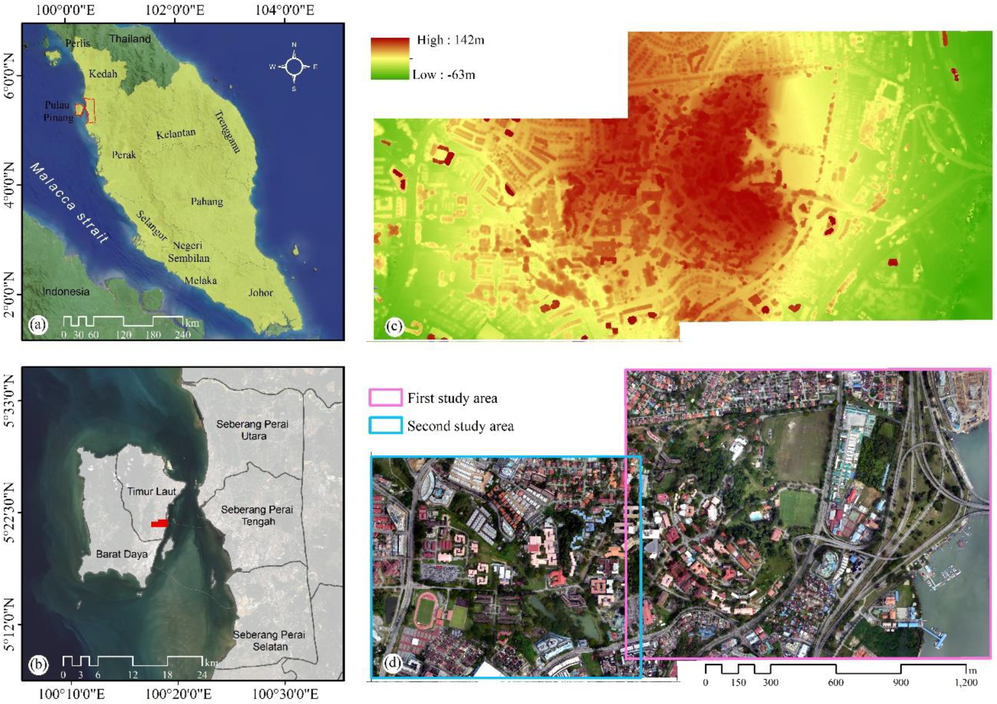
2.1. Study Area
2.2. GT Data
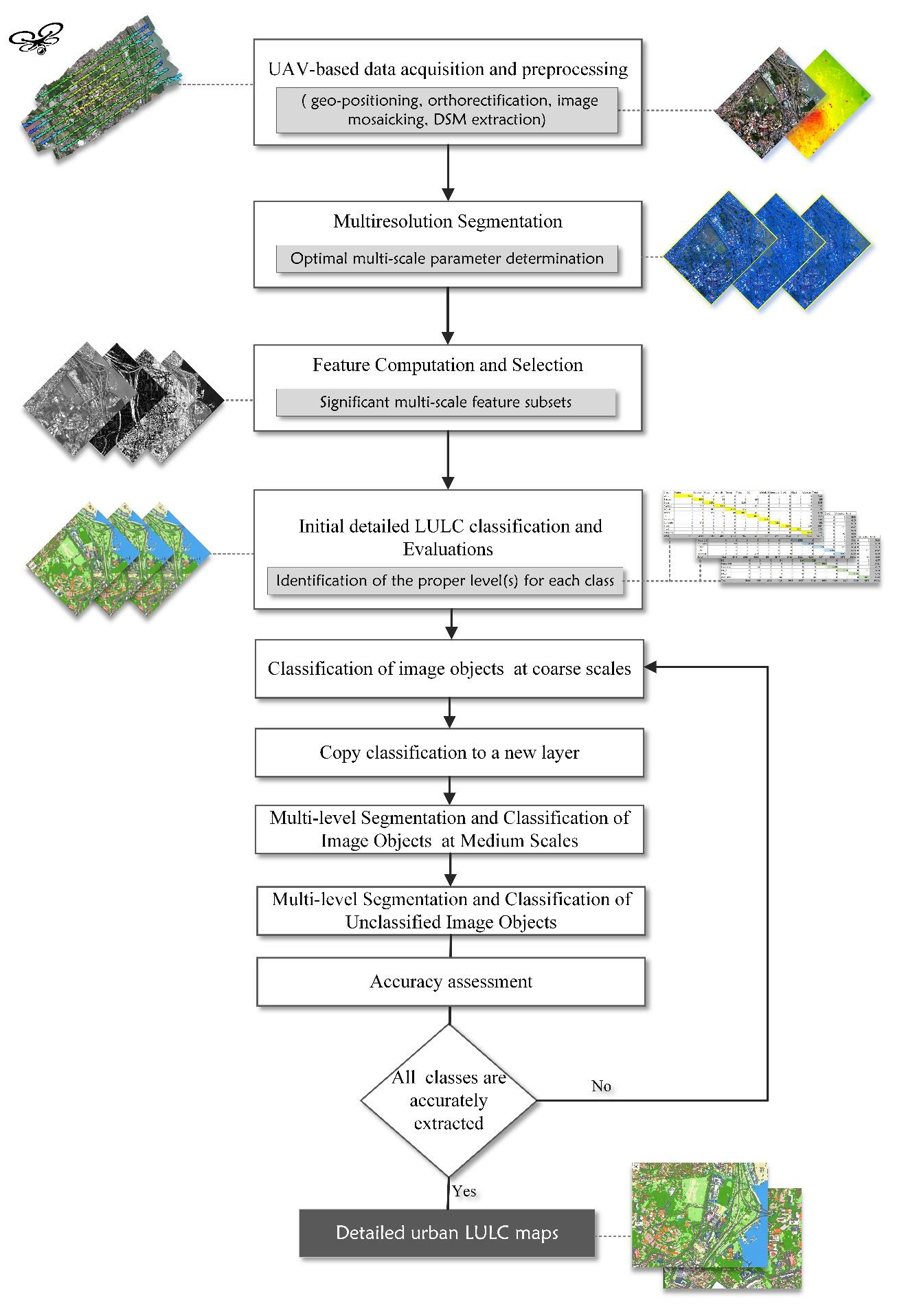
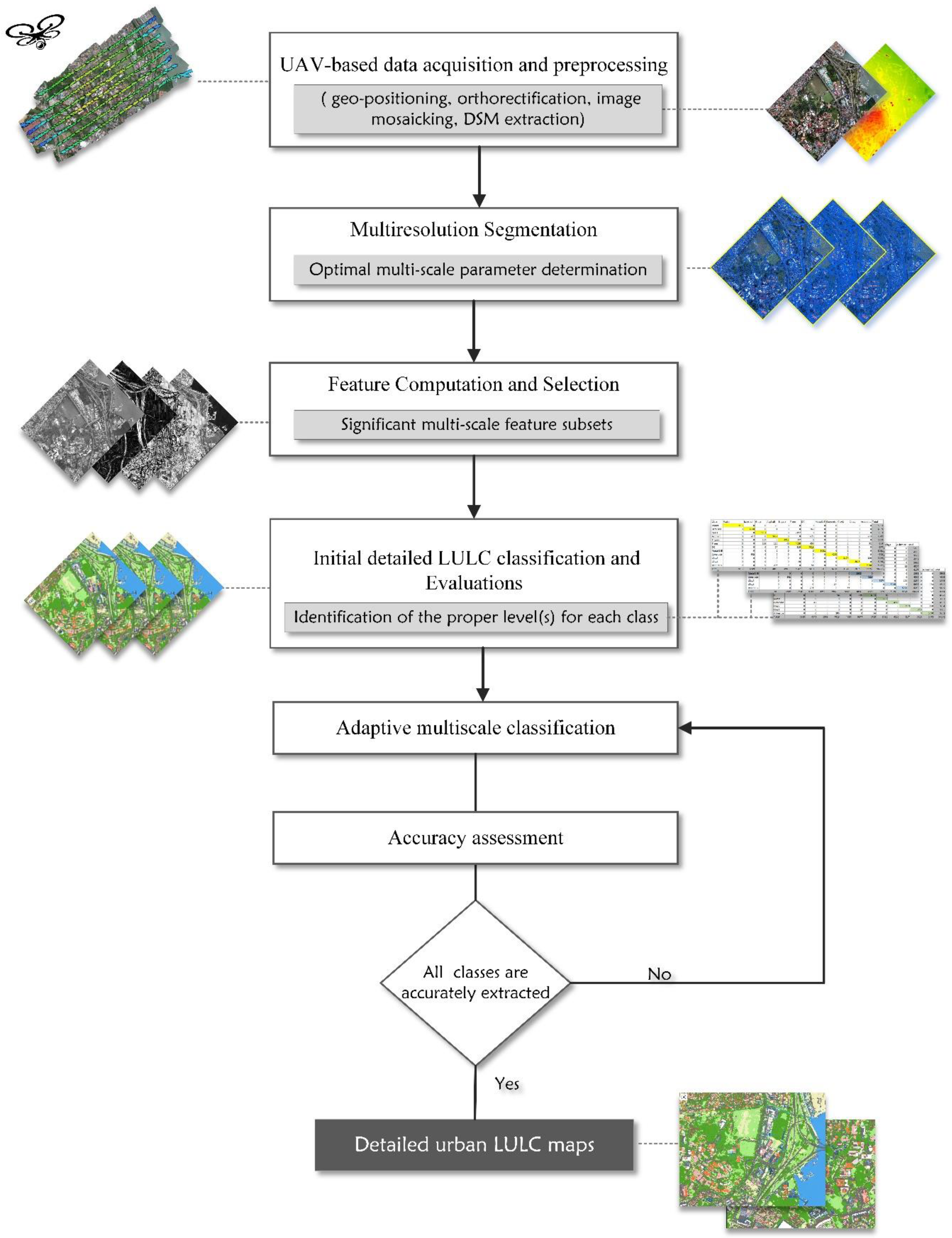
3. Methodology
3.1. Overview
3.2. Image Preprocessing
3.3. MS Image Segmentation Optimization
3.4. Feature Computation and Selection
3.4.1. CFS
3.4.2. SVM
3.5. Supervised MS Image Object Classification
3.6. Evaluation Metrics
3.6.1. OA
3.6.2. K Statistics
3.6.3. Precision, Recall, and F-measure
4. Results
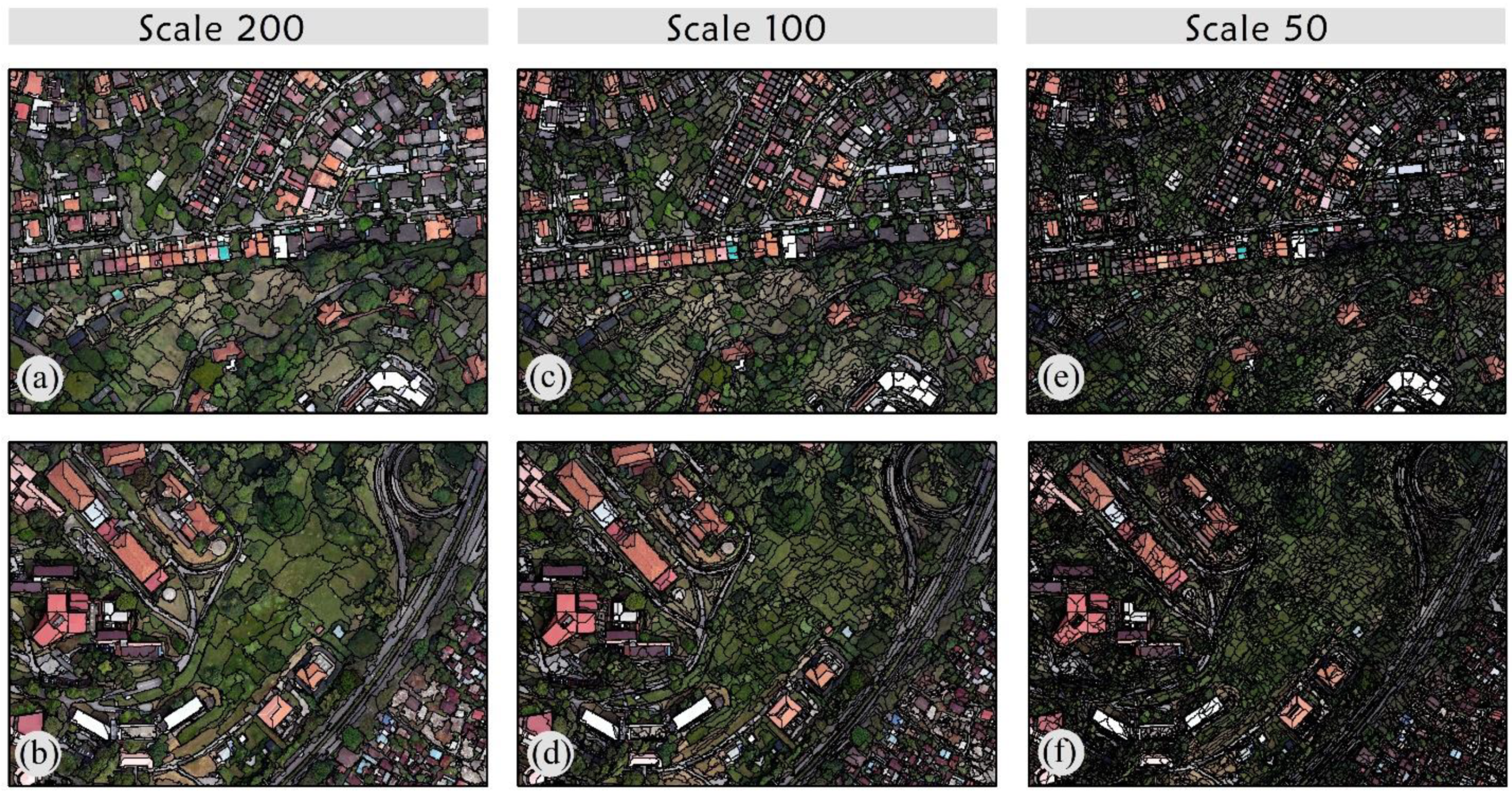
4.1. Results of MS Image Segmentation
4.2. Results of FS
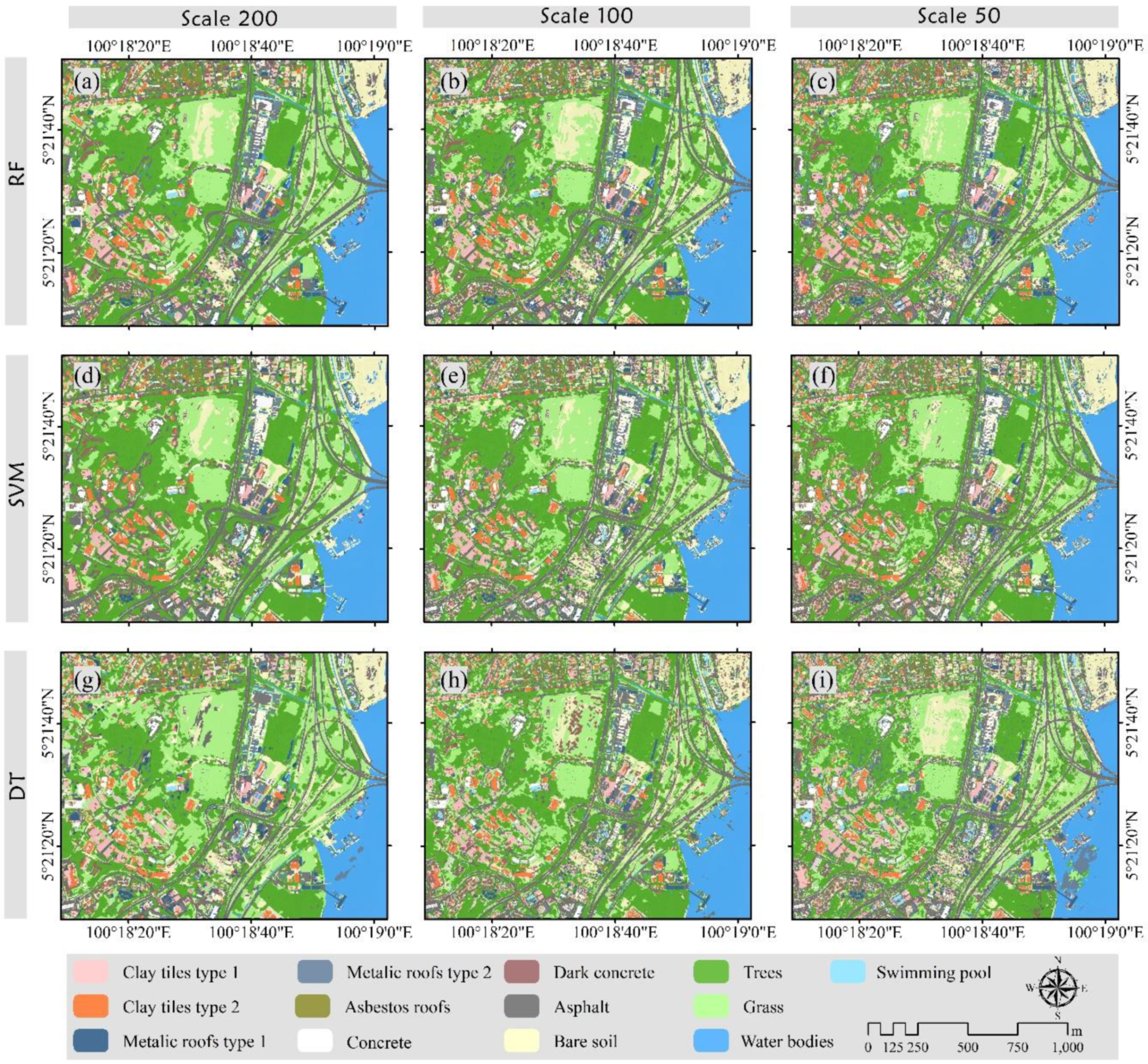
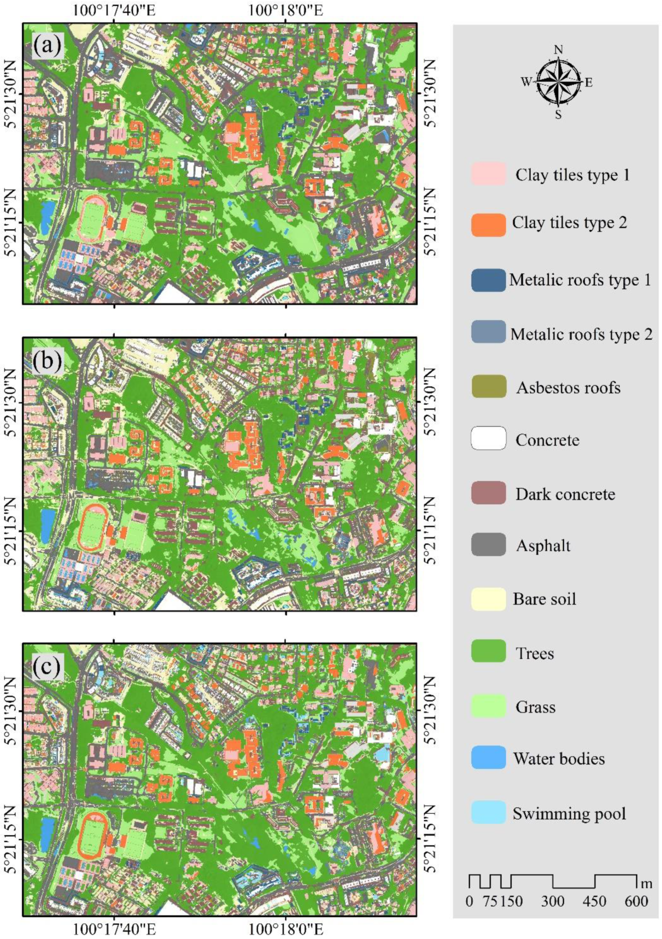
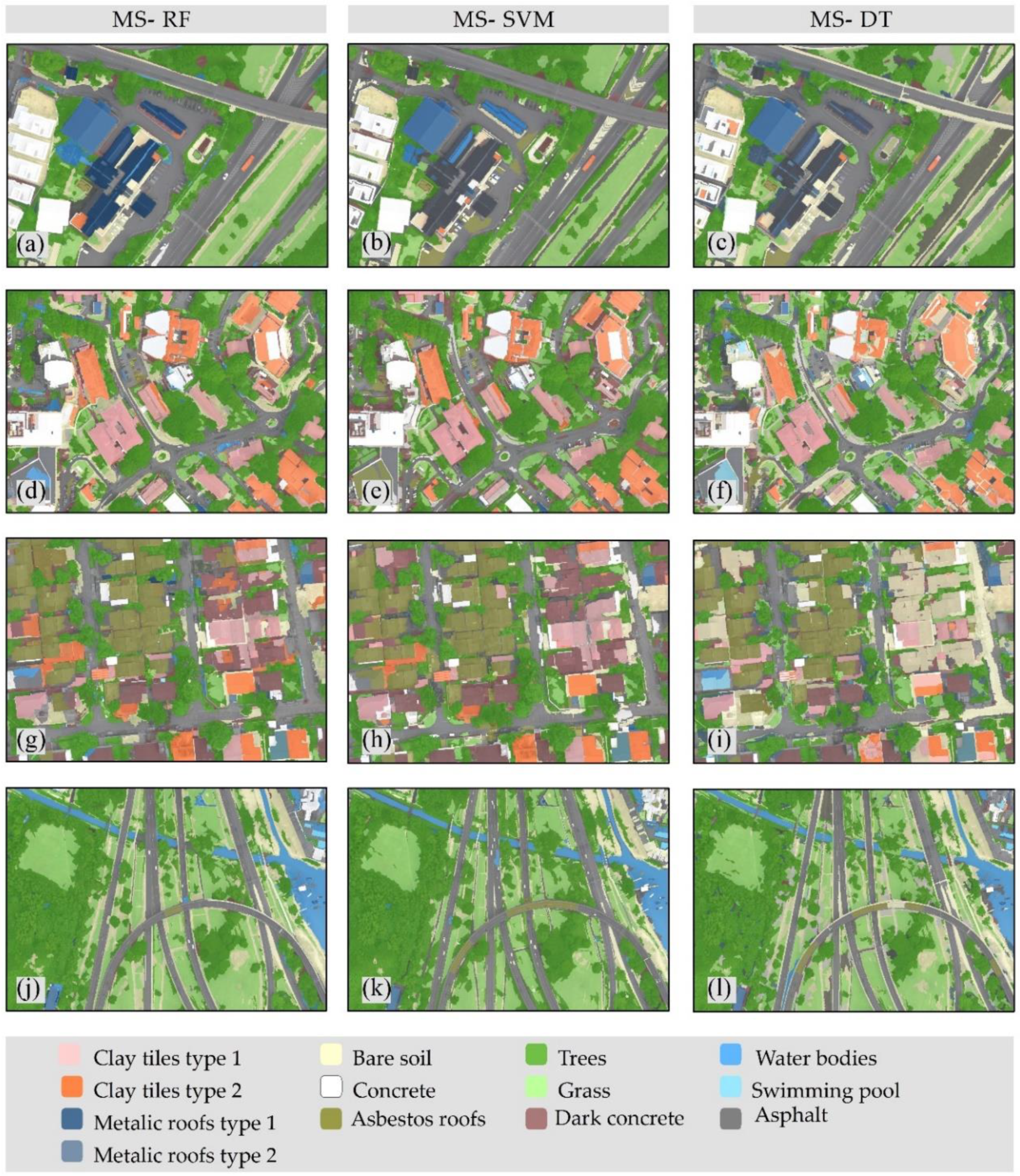
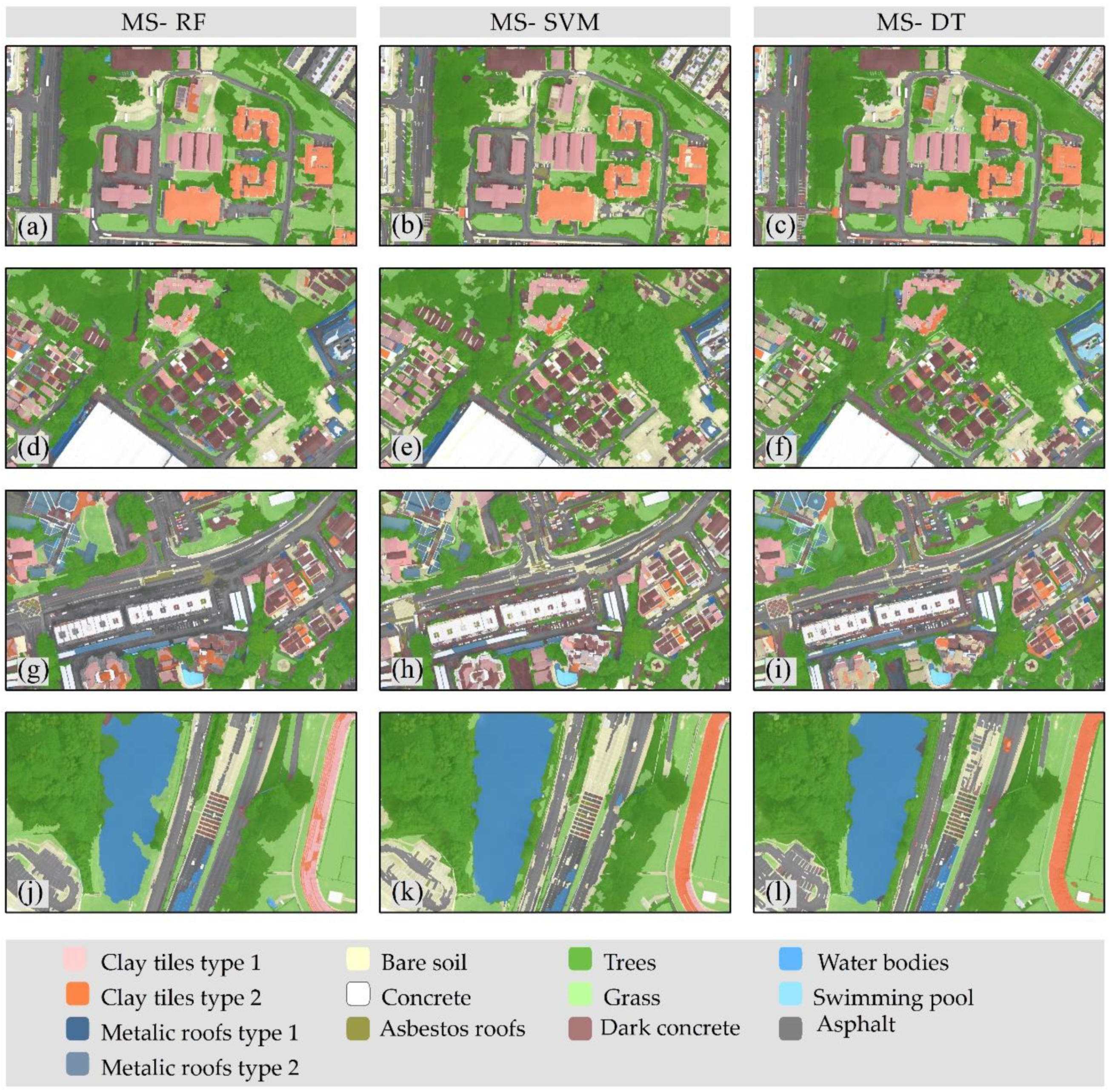
4.3. Classification Results
5. Discussion
6. Conclusions
Author Contributions
Funding
Acknowledgments
Conflicts of Interest
References
- Glade, T. Landslide occurrence as a response to land use change: A review of evidence from New Zealand. Catena 2003, 51, 297–314. [Google Scholar] [CrossRef]
- Scanlon, B.R.; Reedy, R.C.; Stonestrom, D.A.; Prudic, D.E.; Dennehy, K.F. Impact of land use and land cover change on groundwater recharge and quality in the southwestern US. Glob. Chang. Biol. 2005, 11, 1577–1593. [Google Scholar] [CrossRef]
- Bonato, M.; Cian, F.; Giupponi, C. Combining LULC data and agricultural statistics for A better identification and mapping of High nature value farmland: A case study in the veneto Plain, Italy. Land Use Policy 2019, 83, 488–504. [Google Scholar] [CrossRef]
- Acheampong, M.; Yu, Q.; Enomah, L.D.; Anchang, J.; Eduful, M. Land use/cover change in Ghana’s oil city: Assessing the impact of neoliberal economic policies and implications for sustainable development goal number one—A remote sensing and GIS approach. Land Use Policy 2018, 73, 373–384. [Google Scholar] [CrossRef]
- McDowell, R.W.; Snelder, T.; Harris, S.; Lilburne, L.; Larned, S.T.; Scarsbrook, M.; Curtis, A.; Holgate, B.; Phillips, J.; Taylor, K. The land use suitability concept: Introduction and an application of the concept to inform sustainable productivity within environmental constraints. Ecol. Indic. 2018, 91, 212–219. [Google Scholar] [CrossRef]
- Lin, Y.; Jiang, M.; Yao, Y.; Zhang, L.; Lin, J. Use of UAV oblique imaging for the detection of individual trees in residential environments. Urban For. Urban Green. 2015, 14, 404–412. [Google Scholar] [CrossRef]
- Al-najjar, H.A.H.; Kalantar, B.; Pradhan, B.; Saeidi, V. Land cover classification from fused DSM and UAV images using convolutional neural networks. Remote Sens. 2019, 11, 1461. [Google Scholar] [CrossRef]
- Ahmed, O.S.; Shemrock, A.; Chabot, D.; Dillon, C.; Williams, G.; Wasson, R.; Franklin, S.E. Hierarchical land cover and vegetation classification using multispectral data acquired from an unmanned aerial vehicle. Int. J. Remote Sens. 2017, 38, 2037–2052. [Google Scholar] [CrossRef]
- Kalantar, B.; Mansor, S.B.; Sameen, M.I.; Pradhan, B.; Shafri, H.Z.M. Drone-Based land-cover mapping using a fuzzy unordered rule induction algorithm integrated into object-based image analysis. Int. J. Remote Sens. 2017, 38, 2535–2556. [Google Scholar] [CrossRef]
- Zhang, X.; Chen, G.; Wang, W.; Wang, Q.; Dai, F. Object-Based land-cover supervised classification for very-high-resolution UAV images using stacked denoising autoencoders. IEEE J. Sel. Top. Appl. Earth Obs. Remote Sens. 2017, 10, 3373–3385. [Google Scholar] [CrossRef]
- Akar, Ö. Mapping land use with using Rotation Forest algorithm from UAV images. Eur. J. Remote Sens. 2017, 50, 269–279. [Google Scholar] [CrossRef]
- Mancini, A.; Frontoni, E.; Zingaretti, P. A multi/hyper-spectral imaging system for land use/land cover using unmanned aerial systems. In Proceedings of the 2016 International Conference on Unmanned Aircraft Systems (ICUAS), Arlington, VA, USA, 7–10 June 2016; Institute of Electrical and Electronics Engineers (IEEE): Piscataway, NJ, USA, 2016; pp. 1148–1155. [Google Scholar]
- Iizuka, K.; Itoh, M.; Shiodera, S.; Matsubara, T.; Dohar, M.; Watanabe, K. Advantages of unmanned aerial vehicle (UAV) photogrammetry for landscape analysis compared with satellite data: A case study of postmining sites in Indonesia. Cogent Geosci. 2018, 4, 1–15. [Google Scholar] [CrossRef]
- Randall, M.; Fensholt, R.; Zhang, Y.; Jensen, M.B. Geographic object based image analysis of world view-3 imagery for urban hydrologic modelling at the catchment scale. Water 2019, 11, 1133. [Google Scholar] [CrossRef]
- Mboga, N.; Georganos, S.; Grippa, T.; Lennert, M.; Vanhuysse, S.; Wolff, E. Fully convolutional networks and geographic object-based image analysis for the classification of VHR imagery. Remote Sens. 2019, 11, 597. [Google Scholar] [CrossRef]
- Gu, H.; Han, Y.; Yang, Y.; Li, H.; Liu, Z.; Soergel, U.; Blaschke, T.; Cui, S. An efficient parallel multi-scale segmentation method for remote sensing imagery. Remote Sens. 2018, 10, 590. [Google Scholar] [CrossRef]
- Gibril, M.B.A.; Idrees, M.O.; Yao, K.; Shafri, H.Z.M. Integrative image segmentation optimization and machine learning approach for high quality land-use and land-cover mapping using multisource remote sensing data. J. Appl. Remote Sens. 2018, 12, 1. [Google Scholar] [CrossRef]
- De Castro, A.I.; Torres-Sánchez, J.; Peña, J.M.; Jiménez-Brenes, F.M.; Csillik, O.; López-Granados, F. An automatic random forest-OBIA algorithm for early weed mapping between and within crop rows using UAV imagery. Remote Sens. 2018, 10, 285. [Google Scholar] [CrossRef]
- Komárek, J.; Klouček, T.; Prošek, J. The potential of unmanned aerial systems: A tool towards precision classification of hard-to-distinguish vegetation types. Int. J. Appl. Earth Obs. Geoinf. 2018, 71, 9–19. [Google Scholar] [CrossRef]
- Kamal, M.; Kanekaputra, T.; Hermayani, R.; Juniansah, A. Geographic object based image analysis (GEOBIA) for mangrove canopy delineation using aerial photography. IOP Conf. Ser. Earth Environ. Sci. 2019, 313, 12048. [Google Scholar] [CrossRef]
- Mishra, N.; Mainali, K.; Shrestha, B.; Radenz, J.; Karki, D. Species-Level vegetation mapping in a Himalayan treeline ecotone using unmanned aerial system (UAS) imagery. ISPRS Int. J. Geo Inf. 2018, 7, 445. [Google Scholar] [CrossRef]
- White, R.; Bomber, M.; Hupy, J.; Shortridge, A. UAS-GEOBIA approach to sapling identification in jack pine barrens after fire. Drones 2018, 2, 40. [Google Scholar] [CrossRef]
- Gonçalves, J.; Pôças, I.; Marcos, B.; Mücher, C.A.; Honrado, J.P. SegOptim—A new R package for optimizing object-based image analyses of high-spatial resolution remotely-sensed data. Int. J. Appl. Earth Obs. Geoinf. 2019, 76, 218–230. [Google Scholar] [CrossRef]
- Blaschke, T.; Hay, G.J.; Kelly, M.; Lang, S.; Hofmann, P.; Addink, E.; Queiroz Feitosa, R.; Van der Meer, F.; Van der Werff, H.; Van Coillie, F.; et al. Geographic object-based image analysis—Towards a new paradigm. ISPRS J. Photogramm. Remote Sens. 2014, 87, 180–191. [Google Scholar] [CrossRef]
- Ma, L.; Li, M.; Ma, X.; Cheng, L.; Du, P.; Liu, Y. A review of supervised object-based land-cover image classification. ISPRS J. Photogramm. Remote Sens. 2017, 130, 277–293. [Google Scholar] [CrossRef]
- Vincent, L.; Soille, P. Watersheds in digital spaces: An efficient algorithm based on immersion simulations. IEEE Trans. Pattern Anal. Mach. Intell. 1991, 13, 583–598. [Google Scholar] [CrossRef]
- Deren, L.; Zhang, G.; Wu, Z.; Yi, L. An edge embedded marker-based watershed algorithm for high spatial resolution remote sensing image segmentation. IEEE Trans. Image Process. 2010, 19, 2781–2787. [Google Scholar] [CrossRef]
- Benz, U.C.; Hofmann, P.; Willhauck, G.; Lingenfelder, I.; Heynen, M. Multi-Resolution, object-oriented fuzzy analysis of remote sensing data for GIS-ready information. ISPRS J. Photogramm. Remote Sens. 2004, 58, 239–258. [Google Scholar] [CrossRef]
- Comaniciu, D.; Meer, P. Mean shift: A robust approach toward feature space analysis. IEEE Trans. Pattern Anal. Mach. Intell. 2002, 24, 603–619. [Google Scholar] [CrossRef]
- Wang, Y.; Meng, Q.; Qi, Q.; Yang, J.; Liu, Y. Region merging considering within-and between-segment heterogeneity: An improved hybrid remote-sensing image segmentation method. Remote Sens. 2018, 10, 781. [Google Scholar] [CrossRef]
- Kavzoglu, T.; Tonbul, H. A comparative study of segmentation quality for multi-resolution segmentation and watershed transform. In Proceedings of the 8th International Conference on Recent Advances in Space Technologies (RAST), Istanbul, Turkey, 19–22 June 2017; pp. 113–117. [Google Scholar]
- Zhang, X.; Du, S. Learning selfhood scales for urban land cover mapping with very-high-resolution satellite images. Remote Sens. Environ. 2016, 178, 172–190. [Google Scholar] [CrossRef]
- Xiao, P.; Zhang, X.; Zhang, H.; Hu, R.; Feng, X. Multiscale optimized segmentation of urban green cover in high resolution remote sensing image. Remote Sens. 2018, 10, 1813. [Google Scholar] [CrossRef]
- He, Y.; Weng, Q. High Spatial Resolution Remote Sensing: Data, Analysis, and Applications; CRC Press: Boca Raton, FL, USA, 2018; ISBN 9781498767682. [Google Scholar]
- Shen, Y.; Chen, J.; Xiao, L.; Pan, D. Optimizing multiscale segmentation with local spectral heterogeneity measure for high resolution remote sensing images. ISPRS J. Photogramm. Remote Sens. 2019, 157, 13–25. [Google Scholar] [CrossRef]
- Wang, Y.; Qi, Q.; Liu, Y.; Jiang, L.; Wang, J. Unsupervised segmentation parameter selection using the local spatial statistics for remote sensing image segmentation. Int. J. Appl. Earth Obs. Geoinf. 2019, 81, 98–109. [Google Scholar] [CrossRef]
- Drǎguţ, L.; Tiede, D.; Levick, S.R. ESP: A tool to estimate scale parameter for multiresolution image segmentation of remotely sensed data. Int. J. Geogr. Inf. Sci. 2010, 24, 859–871. [Google Scholar] [CrossRef]
- Drǎguţ, L.; Csillik, O.; Eisank, C.; Tiede, D. Automated parameterisation for multi-scale image segmentation on multiple layers. ISPRS J. Photogramm. Remote Sens. 2014, 88, 119–127. [Google Scholar] [CrossRef] [PubMed]
- Johnson, B.; Bragais, M.; Endo, I.; Magcale-Macandog, D.; Macandog, P. Image segmentation parameter optimization considering within-and between-segment heterogeneity at multiple scale levels: Test case for mapping residential areas using landsat imagery. ISPRS Int. J. Geo Inf. 2015, 4, 2292–2305. [Google Scholar] [CrossRef]
- Johnson, B.; Xie, Z. Unsupervised image segmentation evaluation and refinement using a multi-scale approach. ISPRS J. Photogramm. Remote Sens. 2011, 66, 473–483. [Google Scholar] [CrossRef]
- Espindola, G.M.; Camara, G.; Reis, I.A.; Bins, L.S.; Monteiro, A.M. Parameter selection for region-growing image segmentation algorithms using spatial autocorrelation. Int. J. Remote Sens. 2006, 27, 3035–3040. [Google Scholar] [CrossRef]
- Yang, J.; He, Y.; Weng, Q. An automated method to parameterize segmentation scale by enhancing intrasegment homogeneity and intersegment heterogeneity. IEEE Geosci. Remote Sens. Lett. 2015, 12, 1282–1286. [Google Scholar] [CrossRef]
- Ming, D.; Li, J.; Wang, J.; Zhang, M. Scale parameter selection by spatial statistics for GeOBIA: Using mean-shift based multi-scale segmentation as an example. ISPRS J. Photogramm. Remote Sens. 2015, 106, 28–41. [Google Scholar] [CrossRef]
- Yang, J.; Li, P.; He, Y. A multi-band approach to unsupervised scale parameter selection for multi-scale image segmentation. ISPRS J. Photogramm. Remote Sens. 2014, 94, 13–24. [Google Scholar] [CrossRef]
- Kamal, M.; Phinn, S.; Johansen, K. Object-Based approach for multi-scale mangrove composition mapping using multi-resolution image datasets. Remote Sens. 2015, 7, 4753–4783. [Google Scholar] [CrossRef]
- Pedergnana, M.; Marpu, P.R.; Mura, M.D.; Benediktsson, J.A.; Bruzzone, L. A novel technique for optimal feature selection in attribute profiles based on genetic algorithms. IEEE Trans. Geosci. Remote Sens. 2013, 51, 3514–3528. [Google Scholar] [CrossRef]
- Ma, L.; Fu, T.; Blaschke, T.; Li, M.; Tiede, D.; Zhou, Z.; Ma, X.; Chen, D. Evaluation of feature selection methods for object-based land cover mapping of unmanned aerial vehicle imagery using random forest and support vector machine classifiers. ISPRS Int. J. Geo Inf. 2017, 6, 51. [Google Scholar] [CrossRef]
- Martha, T.R.; Kerle, N.; Van Westen, C.J.; Jetten, V.; Kumar, K.V. Segment optimization and data-driven thresholding for knowledge-based landslide detection by object-based image analysis. IEEE Trans. Geosci. Remote Sens. 2011, 49, 4928–4943. [Google Scholar] [CrossRef]
- Ridha, M.; Pradhan, B. An improved algorithm for identifying shallow and deep-seated landslides in dense tropical forest from airborne laser scanning data. Catena 2018, 167, 147–159. [Google Scholar] [CrossRef]
- Al-Ruzouq, R.; Shanableh, A.; Barakat, A.; Gibril, M.; AL-Mansoori, S.; Al-Ruzouq, R.; Shanableh, A.; Barakat, A.; Gibril, M.; AL-Mansoori, S. Image segmentation parameter selection and ant colony optimization for date palm tree detection and mapping from very-high-spatial-resolution aerial imagery. Remote Sens. 2018, 10, 1413. [Google Scholar] [CrossRef]
- Hamedianfar, A.; Gibril, M.B.A. Large-Scale urban mapping using integrated geographic object-based image analysis and artificial bee colony optimization from worldview-3 data. Int. J. Remote Sens. 2019, 40, 6796–6821. [Google Scholar] [CrossRef]
- Hamedianfar, A.; Gibril, M.B.A.; Pellikka, P.K.E. Synergistic use of particle swarm optimization, artificial neural network, and extreme gradient boosting algorithms for urban LULC mapping from WorldView-3 images. Geocart. Int. 2020, 1–19. [Google Scholar] [CrossRef]
- Shanableh, A.; Al-ruzouq, R.; Gibril, M.B.A.; Flesia, C. Spatiotemporal mapping and monitoring of whiting in the semi-enclosed gulf using moderate resolution imaging spectroradiometer (MODIS) time series images and a generic ensemble. Remote Sens. 2019, 11, 1193. [Google Scholar] [CrossRef]
- Shahi, K.; Shafri, H.Z.M.; Hamedianfar, A. Road condition assessment by OBIA and feature selection techniques using very high-resolution WorldView-2 imagery. Geocart. Int. 2017, 32, 1389–1406. [Google Scholar] [CrossRef]
- Cao, J.; Leng, W.; Liu, K.; Liu, L.; He, Z.; Zhu, Y. Object-based mangrove species classification using unmanned aerial vehicle hyperspectral images and digital surface models. Remote Sens. 2018, 10, 89. [Google Scholar] [CrossRef]
- Akar, Ö. The Rotation Forest algorithm and object-based classification method for land use mapping through UAV images. Geocart. Int. 2018, 33, 538–553. [Google Scholar] [CrossRef]
- Liu, L.; Liu, X.; Shi, J.; Li, A. A land cover refined classification method based on the fusion of LiDAR data and UAV image. Adv. Comput. Sci. Res. 2019, 88, 154–162. [Google Scholar] [CrossRef]
- Fotheringham, A.S.; Brunsdon, C.; Charlton, M. Quantitative Geography: Perspectives on Spatial Data Analysis; SAGE: Thousand Oaks, CA, USA, 2000. [Google Scholar]
- Grybas, H.; Melendy, L.; Congalton, R.G. A comparison of unsupervised segmentation parameter optimization approaches using moderate-and high-resolution imagery. GISci. Remote Sens. 2017, 54, 515–533. [Google Scholar] [CrossRef]
- Trimble, T. ECognition Developer 8.7 Reference Book; Trimble Germany GmbH: Munich, Germany, 2011; pp. 319–328. [Google Scholar]
- Gevers, T.; Smeulders, A.W.M. PicToSeek: Combining color and shape invariant features for image retrieval. IEEE Trans. Image Process. 2000, 9, 102–119. [Google Scholar] [CrossRef]
- Sirmacek, B.; Unsalan, C. Building detection from aerial images using invariant color features and shadow information. In Proceedings of the 23rd International Symposium on Computer and Information Sciences, Istanbul, Turkey, 27–29 October 2008; pp. 1–5. [Google Scholar]
- Cretu, A.M.; Payeur, P. Building detection in aerial images based on watershed and visual attention feature descriptors. In Proceedings of the International Conference on Computer and Robot Vision CRV 2013, Regina, SK, Canada, 28–31 May 2013; pp. 265–272. [Google Scholar] [CrossRef]
- Haralick, R.M.; Shanmugam, K.; Dinstein, I. Textural features for image classification. IEEE Trans. Syst. Man Cybern. 1973, 3, 610–621. [Google Scholar] [CrossRef]
- Hall, M.A.; Holmes, G. Benchmarking attribute selection techniques for discrete class data mining. IEEE Trans. Knowl. Data Eng. 2003, 15, 1437–1447. [Google Scholar] [CrossRef]
- Shang, M.; Wang, S.; Zhou, Y.; Du, C.; Liu, W. Object-based image analysis of suburban landscapes using Landsat-8 imagery. Int. J. Digit. Earth 2019, 12, 720–736. [Google Scholar] [CrossRef]
- Al-ruzouq, R.; Shanableh, A.; Mohamed, B.; Kalantar, B. Multi-scale correlation-based feature selection and random forest classification for LULC mapping from the integration of SAR and optical Sentinel imagess. Proc. SPIE 2019, 11157. [Google Scholar] [CrossRef]
- Hall, M.A.; Smith, L.A. Practical feature subset selection for machine learning. In Proceedings of the 21st Australasian Computer Science Conference ACSC’98, Perth, Australia, 4–6 February 1998; Volume 98, pp. 181–191. [Google Scholar]
- Fong, S.; Zhuang, Y.; Tang, R.; Yang, X.; Deb, S. Selecting optimal feature set in high-dimensional data by swarm search. J. Appl. Math. 2013, 2013. [Google Scholar] [CrossRef]
- Raczko, E.; Zagajewski, B. Comparison of support vector machine, random forest and neural network classifiers for tree species classification on airborne hyperspectral APEX images. Eur. J. Remote Sens. 2017, 50, 144–154. [Google Scholar] [CrossRef]
- Tzotsos, A. Preface: A support vector machine for object-based image analysis. In Approach Object Based Image Analysis; Springer: Cham, Switzerland, 2008; Volume 5–8. [Google Scholar] [CrossRef]
- Taner San, B. An evaluation of SVM using polygon-based random sampling inlandslide susceptibility mapping: The Candir catchment area(western Antalya, Turkey). Int. J. Appl. Earth Obs. Geoinf. 2014, 26, 399–412. [Google Scholar] [CrossRef]
- Cortes, C.; Vapnik, V. Support-Vector networks. Mach. Learn. 1995, 20, 273–297. [Google Scholar] [CrossRef]
- Pradhan, B.; Seeni, M.I.; Kalantar, B. Performance evaluation and sensitivity analysis of expert-based, statistical, machine learning, and hybrid models for producing landslide susceptibility maps. In Laser Scanning Applications in Landslide Assessment; Springer International Publishing: Cham, Switzerland, 2017; pp. 193–232. [Google Scholar]
- Pal, M.; Mather, P.M. An assessment of the effectiveness of decision tree methods for land cover classification. Remote Sens. Environ. 2003, 86, 554–565. [Google Scholar] [CrossRef]
- Hamedianfar, A.; Shafri, H.Z.M. Integrated approach using data mining-based decision tree and object-based image analysis for high-resolution urban mapping of WorldView-2 satellite sensor data. J. Appl. Remote Sens. 2016, 10, 025001. [Google Scholar] [CrossRef]
- Pal, M.; Mather, P.M. Decision tree based classification of remotely sensed data. In Proceedings of the 22nd Asian Conference on Remote Sensing, Singapore, 5–9 November 2001; p. 9. [Google Scholar]
- Eisavi, V.; Homayouni, S.; Yazdi, A.M.; Alimohammadi, A. Land cover mapping based on random forest classification of multitemporal spectral and thermal images. Environ. Monit. Assess. 2015, 187, 1–14. [Google Scholar] [CrossRef]
- Berhane, T.M.; Lane, C.R.; Wu, Q.; Autrey, B.C.; Anenkhonov, O.A.; Chepinoga, V.V.; Liu, H. Decision-Tree, rule-based, and random forest classification of high-resolution multispectral imagery for wetland mapping and inventory. Remote Sens. 2018, 10, 580. [Google Scholar] [CrossRef]
- Goetz, J.N.; Brenning, A.; Petschko, H.; Leopold, P. Computers & geosciences evaluating machine learning and statistical prediction techniques for landslide susceptibility modeling. Comput. Geosci. 2015, 81, 1–11. [Google Scholar] [CrossRef]
- Tian, S.; Zhang, X.; Tian, J.; Sun, Q. Random forest classification of wetland landcovers from multi-sensor data in the arid region of Xinjiang, China. Remote Sens. 2016, 8, 954. [Google Scholar] [CrossRef]
- Zerrouki, N.; Bouchaffra, D. Pixel-based or object-based: Which approach is more appropriate for remote sensing image classification? In Proceedings of the IEEE International Conference on Systems, Man, and Cybernetics (SMC), San Diego, CA, USA, 5–8 October 2014; Volume 2014, pp. 864–869. [Google Scholar]
- Li, W.; Guo, Q. A new accuracy assessment method for one-class remote sensing classification. IEEE Trans. Geosci. Remote Sens. 2014, 52, 4621–4632. [Google Scholar] [CrossRef]
- Millard, K.; Richardson, M. On the importance of training data sample selection in random forest image classification: A case study in peatland ecosystem mapping. Remote Sens. 2015, 7, 8489–8515. [Google Scholar] [CrossRef]


| LULC Type | Images | Description |
|---|---|---|
| Water bodies |  | Water bodies with light blue and green colors |
| Trees and grass |  | Various tree species and grass thickness |
| Bare soil |  | Exposed soil with different colors |
| Concrete roofs |  | Concrete slab with bright white color |
| Dark concrete roofs |  | Residential and industrial buildings with dark brown color |
| Clay tiles type 1 |  | Roofing material with different structural shapes and red color |
| Clay tiles type 2 |  | Roofing material with different structures and bright peach color |
| Asbestos cement roofs |  | Roofs with regular shape and grey color |
| Metallic roofs type 1 |  | Metal deck with blue color |
| Metallic roofs type 2 |  | Rooftops with turquoise color |
| Roads |  | Urban roads with grey color |
| Feature Type | Tested Feature Name | Description | Reference |
|---|---|---|---|
| Spectral | Mean | The mean intensity values computed for an image segment of the RGB channels and the DSM | [60] |
| Standard deviation | The standard deviation values computed for an image segment of the RGM channels and the DSM. | [60] | |
| Max_ difference | The maximum difference between the RGB channels. | [60] | |
| Brightness | The average of means of the RGB channels. | [60] | |
| NDRG | [61] | ||
| NDGB | [61] | ||
| NDBG | [61] | ||
| NDRB | [61] | ||
| NDBR | [61] | ||
| NDGR | [61] | ||
| RB | [61] | ||
| Ratio-R | [61] | ||
| Ratio-G | [61] | ||
| Ratio-B | [61] | ||
| V | [62] | ||
| S | [63] | ||
| Texture | Mean | The grey level co-occurrence matrix (GLCM) mean sum of all directions determined for each band from the RGB channels and the DSM. | [64] |
| Homogeneity | The GLCM homogeneity sum of all directions determined for each band from the RGB channels, and the DSM. | [64] | |
| Contrast | The GLCM contrast sum of all directions determined for each band from the RGB channels, and the DSM. The grey level difference vector (GLDV) matrix contrast sum of all directions determined for each band from the RGB channels, and the DSM. | [64] | |
| Entropy | The GLCM and GLDV entropy sum of all directions determined for each band from the RGB channels, and the DSM. | [64] | |
| Correlation | The GLCM correlation sum of all directions determined for each band from the RGB channels, and the DSM. | [64] | |
| Standard deviation | The GLCM standard deviation sum of all directions determined for each band from the RGB channels, and the DSM. | [64] | |
| Dissimilarity | The GLCM dissimilarity sum of all directions determined for each band from the RGB channels, and the DSM. | [64] | |
| Angular second moment | The GLCM angular second-moment sum of all directions determined for each band from the RGB channels, and the DSM. | [64] | |
| Geometric | Length\Width | The ratio between the length and width. | [60] |
| Rectangular Fit | A ratio that is based on how well an image object fits into a rectangle. | [60] | |
| Shape_index | A ratio that defines border smoothness of image objects and can be computed by dividing the border length of an image object by four times the square root of its area. | [60] | |
| Density | It can be computed by dividing the area covered by an image object by its radius. | [60] | |
| Elliptic_fit | A ratio based on how well an image object can fit into an ellipse. | [60] | |
| Compactness | It is expressed as the ratio of the area of an image object to the area of a circle with a similar perimeter. | [60] |
| Scale | No of Objects | WV mean | MI mean | WV norm | MI norm | F-Measure | ||
|---|---|---|---|---|---|---|---|---|
| = 3 | = 1 | = 0.33 | ||||||
| 25 | 340731 | 78.606 | 0.548 | 1.000 | 0.000 | 0 | 0 | 0 |
| 50 | 104840 | 132.924 | 0.452 | 0.858 | 0.242 | 0.684 | 0.377 | 0.260 |
| 75 | 53011 | 178.661 | 0.395 | 0.739 | 0.385 | 0.677 | 0.506 | 0.404 |
| 100 | 33217 | 217.177 | 0.344 | 0.639 | 0.514 | 0.624 | 0.570 | 0.524 |
| 125 | 22978 | 253.258 | 0.314 | 0.545 | 0.588 | 0.549 | 0.566 | 0.584 |
| 150 | 16878 | 288.418 | 0.286 | 0.453 | 0.658 | 0.468 | 0.537 | 0.630 |
| 175 | 12887 | 322.978 | 0.250 | 0.363 | 0.748 | 0.383 | 0.489 | 0.674 |
| 200 | 10181 | 354.309 | 0.229 | 0.281 | 0.801 | 0.301 | 0.416 | 0.678 |
| 225 | 8216 | 384.925 | 0.217 | 0.202 | 0.833 | 0.218 | 0.325 | 0.637 |
| 250 | 6841 | 412.203 | 0.195 | 0.130 | 0.888 | 0.143 | 0.227 | 0.566 |
| 275 | 5738 | 439.515 | 0.169 | 0.059 | 0.953 | 0.065 | 0.112 | 0.384 |
| 300 | 4961 | 462.250 | 0.150 | 0.000 | 1.000 | 0 | 0 | 0 |
| Scale | Feature Type | CFS | SVM | ||||||
|---|---|---|---|---|---|---|---|---|---|
| Selected Features | No | OA | K | Selected Features | No | OA | K | ||
| 50 | Spectral | Red, Blue, DSM, SD_DSM, Vegetation, Ratio_G, Ratio_B, NDRG, NDGR NDBR, Max_diff | 16 | 91.63 | 0.93 | Red, Green, Blue, DSM, Vegetation, Ratio_G, Ratio_B, NDGR, NDBR, NDRB, NDGB, NDBG, Shadow, RB, Max_diff, | 21 | 91.61 | 0.91 |
| Textural | GLCM_Mean_DSM, GLCM_Entropy_Green, GLCM_ Dissimilarity _Blue, GLCM_SD_Blue | GLCM_ Entropy _R, GLCM_ Entropy _Blue, GLCM_ Entropy _Green, GLCM_ Homogeneity _Red, GLDV_Mean_Blue | |||||||
| Geometrical | Shape_index | Length/Width | |||||||
| 100 | Spectral | Red, Green, Blue, DSM, SD_DSM, SD_R, Vegetation, Ratio_R, Ratio_G, NDRG, NDBR, NDBG, Shadow, RB, Max_diff, | 22 | 93.3 | 0.92 | Green, Red, Blue, DSM, Vegetation, Ratio_G, Ratio_Blue, NDRG, NDGR, NDGB, RB, NDBR, NDRB, Shadow, NDBG, Max_diff, Brightness | 28 | 92.11 | 0.914 |
| Textural | GLCM_Mean_Red, GLCM_Mean_DSM, GLCM_SD_Green, GLCM_Correlation_DSM, GLCM_ Dissimilarity _Blue, GLCM_Ang 2nd moment_Green | GLCM_Mean_DSM, GLCM_Mean_Blue, GLCM_ Entropy _Blue, GLCM_ Entropy _Red, GLCM_ Entropy _Green, GLCM_ Homogeneity _Red, GLDV_Mean_Blue, GLDV_Conrast_Blue, GLDV_Entropy_Red. | |||||||
| Geometrical | Shape_index | Shape_index, Length/Width | |||||||
| 200 | Spectral | Red, Green, Blue, DSM, SD_DSM, Vegetation, Ratio_R, Ratio_G, Ratio_B, NDRG, NDGR, NDBR, NDGB, NDRB, Shadow Max_diff, | 27 | 93.78 | 0.93 | Red, Green, Blue, DSM, SD_DSM, Vegetation, Ratio_G, Ratio_B, NDGR, NDBG, Shadow, RB, Max_diff | 21 | 92.3 | 0.92 |
| Textural | GLCM_Mean_Red, GLCM_Mean_Blue, GLCM_SD_DSM, GLCM_SD_Green, GLCM_ Homogeneity _DSM, GLCM_Ang 2nd moment _Blue, GLCM_ Dissimilarity _Blue, GLCM_ Correlation _Rede, GLCM_ Homogeneity _Red | GLCM_Mean_Blue, GLCM_ Homogeneity _Green, GLCM_Entropy_R, GLCM_ Correlation _Blue, GLDV_Mean_Blue, GLDV_Entropy_DSM | |||||||
| Geometrical | Shape_index, Length/Width | Length/Width, Compactness | |||||||
| SS-RF | |||||||||
|---|---|---|---|---|---|---|---|---|---|
| Class | SP 200 | SP 100 | SP 50 | ||||||
| Precision | Recall | F-Measure | Precision | Recall | F-Measure | Precision | Recall | F-Measure | |
| Water bodies | 1.000 | 0.980 | 0.990 | 1.000 | 0.997 | 0.999 | 1.000 | 0.997 | 0.999 |
| Bare soil | 0.879 | 0.918 | 0.898 | 0.653 | 0.404 | 0.499 | 0.850 | 0.942 | 0.893 |
| Grass | 0.790 | 0.352 | 0.487 | 0.871 | 0.878 | 0.874 | 0.871 | 0.994 | 0.928 |
| Asphalt | 0.855 | 0.757 | 0.803 | 0.674 | 0.626 | 0.649 | 0.771 | 0.569 | 0.655 |
| Metallic roofs 2 | 0.992 | 0.862 | 0.922 | 1.000 | 0.924 | 0.961 | 1.000 | 1.000 | 1.000 |
| Trees | 0.580 | 0.830 | 0.683 | 0.790 | 0.999 | 0.883 | 0.999 | 0.973 | 0.986 |
| Dark concrete | 0.741 | 0.961 | 0.836 | 1.000 | 0.899 | 0.947 | 0.994 | 0.969 | 0.981 |
| Metallic roofs 1 | 1.000 | 1.000 | 1.000 | 1.000 | 1.000 | 1.000 | 1.000 | 1.000 | 1.000 |
| Concrete | 1.000 | 0.925 | 0.961 | 1.000 | 0.906 | 0.951 | 0.983 | 0.914 | 0.947 |
| Clay tiles type 2 | 1.000 | 0.964 | 0.981 | 0.980 | 0.874 | 0.924 | 0.985 | 0.983 | 0.984 |
| Clay tiles type 1 | 1.000 | 0.996 | 0.998 | 0.474 | 0.902 | 0.621 | 0.977 | 1.000 | 0.989 |
| Asbestos | 0.913 | 0.951 | 0.932 | 0.743 | 0.838 | 0.788 | 0.624 | 0.849 | 0.719 |
| OA | 88.4% | 84.25% | 92.2% | ||||||
| Kappa | 0.873 | 0.827 | 0.914 | ||||||
| SS-SVM | |||||||||
| Water bodies | 0.964 | 1.000 | 0.982 | 1.000 | 0.998 | 0.999 | 1.000 | 1.000 | 1.000 |
| Bare soil | 0.861 | 0.823 | 0.842 | 0.940 | 0.974 | 0.956 | 0.936 | 1.000 | 0.967 |
| Grass | 0.790 | 0.742 | 0.765 | 0.787 | 0.866 | 0.825 | 0.835 | 0.874 | 0.854 |
| Asphalt | 0.861 | 0.836 | 0.849 | 0.906 | 0.854 | 0.879 | 0.878 | 0.745 | 0.806 |
| Metallic roofs 2 | 0.854 | 1.000 | 0.921 | 0.891 | 1.000 | 0.942 | 0.998 | 1.000 | 0.999 |
| Trees | 0.943 | 0.939 | 0.941 | 0.941 | 0.953 | 0.947 | 0.974 | 0.963 | 0.969 |
| Dark concrete | 0.835 | 0.624 | 0.714 | 0.999 | 0.651 | 0.788 | 0.977 | 0.633 | 0.768 |
| Metallic roofs 1 | 0.969 | 0.808 | 0.881 | 1.000 | 0.848 | 0.918 | 1.000 | 1.000 | 1.000 |
| Concrete | 1.000 | 0.907 | 0.951 | 1.000 | 0.993 | 0.996 | 1.000 | 0.942 | 0.970 |
| Clay tiles type 2 | 1.000 | 1.000 | 1.000 | 1.000 | 1.000 | 1.000 | 0.928 | 0.982 | 0.954 |
| Clay tiles type 1 | 0.485 | 0.992 | 0.651 | 0.485 | 0.911 | 0.633 | 0.474 | 0.873 | 0.614 |
| Asbestos | 0.983 | 0.933 | 0.958 | 0.889 | 0.967 | 0.926 | 0.750 | 0.952 | 0.839 |
| OA | 88% | 90.5% | 89.7% | ||||||
| Kappa | 0.868 | 0.896 | 0.886 | ||||||
| SS-DT | |||||||||
| Water bodies | 1.000 | 0.788 | 0.881 | 1.000 | 1.000 | 1.000 | 0.915 | 1.000 | 0.956 |
| Bare soil | 0.889 | 0.853 | 0.871 | 0.758 | 0.886 | 0.817 | 0.729 | 0.924 | 0.815 |
| Grass | 0.790 | 0.246 | 0.375 | 0.871 | 0.244 | 0.381 | 0.864 | 0.687 | 0.765 |
| Asphalt | 0.752 | 0.812 | 0.781 | 0.707 | 0.677 | 0.692 | 0.710 | 0.541 | 0.614 |
| Metallic roofs 2 | 0.957 | 0.858 | 0.905 | 0.998 | 1.000 | 0.999 | 0.998 | 0.846 | 0.916 |
| Trees | 0.529 | 0.895 | 0.665 | 0.806 | 0.945 | 0.870 | 0.904 | 0.965 | 0.934 |
| Dark concrete | 0.732 | 0.966 | 0.833 | 0.946 | 0.843 | 0.891 | 0.943 | 0.925 | 0.934 |
| Metallic roofs 1 | 1.000 | 0.964 | 0.982 | 1.000 | 1.000 | 1.000 | 1.000 | 1.000 | 1.000 |
| Concrete | 1.000 | 0.925 | 0.961 | 0.983 | 0.911 | 0.946 | 0.975 | 1.000 | 0.987 |
| Clay tiles type 2 | 0.948 | 0.521 | 0.672 | 0.886 | 0.902 | 0.894 | 1.000 | 0.823 | 0.903 |
| Clay tiles type 1 | 0.474 | 0.948 | 0.632 | 0.385 | 0.882 | 0.536 | 1.000 | 1.000 | 1.000 |
| Asbestos | 0.676 | 1.000 | 0.806 | 0.756 | 0.833 | 0.793 | 0.639 | 0.852 | 0.730 |
| OA | 79% | 83.4% | 88.1% | ||||||
| K | 0.771 | 0.819 | 0.869 | ||||||
| MS-RF | MS-SVM | MS-DT | |||||||
|---|---|---|---|---|---|---|---|---|---|
| Class | Precision | Recall | F-Measure | Precision | Recall | F-Measure | Precision | Recall | F-Measure |
| Water bodies | 1.000 | 0.967 | 0.983 | 1.000 | 0.998 | 0.999 | 1.000 | 1.000 | 1.000 |
| Bare soil | 0.761 | 0.754 | 0.757 | 0.919 | 1.000 | 0.958 | 0.899 | 0.810 | 0.852 |
| Grass | 0.871 | 0.933 | 0.901 | 0.996 | 0.892 | 0.941 | 0.869 | 0.698 | 0.774 |
| Asphalt | 0.863 | 0.916 | 0.889 | 0.851 | 0.944 | 0.895 | 0.765 | 0.705 | 0.734 |
| Metallic roofs 2 | 1.000 | 0.999 | 1.000 | 0.998 | 1.000 | 0.999 | 0.998 | 0.873 | 0.932 |
| Trees | 0.972 | 0.972 | 0.972 | 0.941 | 0.999 | 0.969 | 0.888 | 0.999 | 0.940 |
| Dark concrete | 0.832 | 0.963 | 0.893 | 0.996 | 0.646 | 0.783 | 0.768 | 0.950 | 0.849 |
| Metallic roofs 1 | 1.000 | 1.000 | 1.000 | 1.000 | 1.000 | 1.000 | 1.000 | 1.000 | 1.000 |
| Concrete | 1.000 | 0.925 | 0.961 | 1.000 | 0.993 | 0.996 | 0.975 | 1.000 | 0.987 |
| Clay tiles type 2 | 1.000 | 0.964 | 0.981 | 1.000 | 1.000 | 1.000 | 0.931 | 0.878 | 0.904 |
| Clay tiles type 1 | 1.000 | 0.923 | 0.960 | 0.485 | 0.904 | 0.631 | 1.000 | 1.000 | 1.000 |
| Asbestos | 0.962 | 0.969 | 0.966 | 0.983 | 0.927 | 0.955 | 0.935 | 0.975 | 0.954 |
| OA | 94.40% | 92.50% | 91.60% | ||||||
| K | 0.938 | 0.917 | 0.908 | ||||||
| RF | SVM | DT | |||||||
|---|---|---|---|---|---|---|---|---|---|
| Class | Precision | Recall | F-Measure | Precision | Recall | F-Measure | Precision | Recall | F-Measure |
| Water bodies | 0.531 | 0.989 | 0.691 | 0.594 | 0.969 | 0.737 | 0.585 | 0.974 | 0.731 |
| Bare soil | 0.960 | 0.884 | 0.921 | 0.982 | 0.960 | 0.971 | 0.953 | 0.788 | 0.862 |
| Grass | 0.972 | 0.650 | 0.779 | 0.984 | 0.786 | 0.874 | 0.912 | 1.000 | 0.954 |
| Asphalt | 0.925 | 1.000 | 0.961 | 0.976 | 1.000 | 0.988 | 0.973 | 1.000 | 0.986 |
| Metallic roofs 2 | 1.000 | 1.000 | 1.000 | 0.969 | 0.680 | 0.800 | 0.745 | 1.000 | 0.854 |
| Trees | 1.000 | 0.959 | 0.979 | 1.000 | 0.984 | 0.992 | 1.000 | 0.618 | 0.764 |
| Dark concrete | 0.971 | 0.975 | 0.973 | 0.992 | 1.000 | 0.996 | 0.901 | 0.990 | 0.944 |
| Metallic roofs 1 | 0.992 | 1.000 | 0.996 | 0.980 | 1.000 | 0.990 | 0.986 | 1.000 | 0.993 |
| Concrete | 0.953 | 1.000 | 0.976 | 1.000 | 1.000 | 1.000 | 0.953 | 1.000 | 0.976 |
| Clay tiles type 2 | 1.000 | 0.961 | 0.980 | 1.000 | 0.983 | 0.991 | 1.000 | 0.856 | 0.923 |
| Clay tiles type 1 | 1.000 | 1.000 | 1.000 | 1.000 | 1.000 | 1.000 | 1.000 | 1.000 | 1.000 |
| OA | 92.46% | 94.45% | 90.46% | ||||||
| K | 0.916 | 0.938 | 0.893 | ||||||
© 2020 by the authors. Licensee MDPI, Basel, Switzerland. This article is an open access article distributed under the terms and conditions of the Creative Commons Attribution (CC BY) license (http://creativecommons.org/licenses/by/4.0/).
Share and Cite
Gibril, M.B.A.; Kalantar, B.; Al-Ruzouq, R.; Ueda, N.; Saeidi, V.; Shanableh, A.; Mansor, S.; Shafri, H.Z.M. Mapping Heterogeneous Urban Landscapes from the Fusion of Digital Surface Model and Unmanned Aerial Vehicle-Based Images Using Adaptive Multiscale Image Segmentation and Classification. Remote Sens. 2020, 12, 1081. https://doi.org/10.3390/rs12071081
Gibril MBA, Kalantar B, Al-Ruzouq R, Ueda N, Saeidi V, Shanableh A, Mansor S, Shafri HZM. Mapping Heterogeneous Urban Landscapes from the Fusion of Digital Surface Model and Unmanned Aerial Vehicle-Based Images Using Adaptive Multiscale Image Segmentation and Classification. Remote Sensing. 2020; 12(7):1081. https://doi.org/10.3390/rs12071081
Chicago/Turabian StyleGibril, Mohamed Barakat A., Bahareh Kalantar, Rami Al-Ruzouq, Naonori Ueda, Vahideh Saeidi, Abdallah Shanableh, Shattri Mansor, and Helmi Z. M. Shafri. 2020. "Mapping Heterogeneous Urban Landscapes from the Fusion of Digital Surface Model and Unmanned Aerial Vehicle-Based Images Using Adaptive Multiscale Image Segmentation and Classification" Remote Sensing 12, no. 7: 1081. https://doi.org/10.3390/rs12071081
APA StyleGibril, M. B. A., Kalantar, B., Al-Ruzouq, R., Ueda, N., Saeidi, V., Shanableh, A., Mansor, S., & Shafri, H. Z. M. (2020). Mapping Heterogeneous Urban Landscapes from the Fusion of Digital Surface Model and Unmanned Aerial Vehicle-Based Images Using Adaptive Multiscale Image Segmentation and Classification. Remote Sensing, 12(7), 1081. https://doi.org/10.3390/rs12071081